SHIP EMISSION INFLUENCE ON CLOUDS: A STUDY USING SATELLITE RETRIEVED
CLOUD PROPERTIES
Karsten Peters1,2, Johannes Quaas1, Irina Sandu1, Bjorn Stevens1, and Hartmut Grassl1 1
Max-Planck-Institut f¨ur Meteorologie, Bundesstrasse 53, 20146 Hamburg, Germany
2International Max Planck Research School on Earth System Modelling, Bundesstrasse 53, 20146 Hamburg, Germany
ABSTRACT
In this study, we propose a statistical method to evalu-ate scenes in which ship emission influence on clouds could be observed. This method aims at efficiently sep-arating clean and polluted marine boundary layer (MBL) air masses. A ship emission inventory is used to find re-gions where significant spatial contrast in shipping emis-sions is present. The regions selected are located in the southeastern Pacific as well as in the mid- and southeast-ern Atlantic. We use MBL-wind trajectories from 2002 through 2007 to select scenes which have the potential to offer a clear separation of clean and polluted air masses. The statistical analysis of satellite retrieved cloud- and aerosol properties does not reveal a depictable effect of ship emissions on the either or the other. We propose that this is due to the small statistical sample sizes, un-certainties in the method adopted and the smallness of ship emissions in general.
Key words: ship emissions; aerosol indirect effects; satel-lite measurements.
1. INTRODUCTION
Anthropogenic activities come in hand with emissions of aerosols and aerosol precursor gases, making the quan-tification of their impact on cloud properties, e.g. cloud droplet number concentration [Twomey, 1974, Lohmann and Feichter, 2005], cloud lifetime [Albrecht, 1989, Stevens and Feingold, 2009] or even cloud top height [Koren et al., 2005, Teller and Levin, 2006], a topic of ongoing research. These aerosol effects on cloud micro-and macrophysical properties are referred to as aerosol indirect effects and are subject to the largest uncertainties of all radiative forcing components of the Earth System when it comes to assessing human induced climate forc-ing [Forster et al., 2007].
Seagoing ships are the least regulated sources of anthro-pogenic emissions. Combustion of such fuels produces, aside from gaseous species, large amounts of particulate matter (PM) consisting of elemental (black) and organic carbon, sulfate, ash and particles forming from sulfuric
acid [Petzold et al., 2008, and references therein]. Given that conditions for aerosol-cloud-interactions at the top of the marine boundary layer (MBL) are fulfilled, a certain number of emitted particles can serve as cloud conden-sation nuclei, leading to aerosol indirect effects [Hobbs et al., 2000, Petzold et al., 2005, Dusek et al., 2006, Pet-zold et al., 2008]. A number of experimental and ob-servational studies have have been performed to iden-tify and quaniden-tify the underlying processes and their ef-fect on cloud micro- and macrophysical properties [Frick and Hoppel, 2000, Durkee et al., 2000, Devasthale et al., 2006, Petzold et al., 2008]. Results of the studies using satellite data show that it is feasible to attribute changes in cloud properties to ship emissions [Schreier et al., 2006, 2007, Campmany et al., 2009].
In this study, we propose a new approach towards quan-tifying the effect of ship emissions on clouds at a larger scale. We aim at sampling clean and polluted maritime regions of identical large scale meteorology. This is es-pecially important because cloud properties and their sus-ceptibility towards changes in anthropogenic aerosol are believed to be regime dependent [Stevens and Feingold, 2009]. We then perform a statistical analysis of satel-lite retrieved cloud- and aerosol properties with respect to clean and polluted environments.
The method and data are described in section 2 and the results in section 3. A discussion of the results and an outlook are given in section 4.
2. METHOD AND DATA
We use a combination of datasets to characterise scenes which are suited for the analysis of ship emission influ-ence on clouds in a statistical sense.
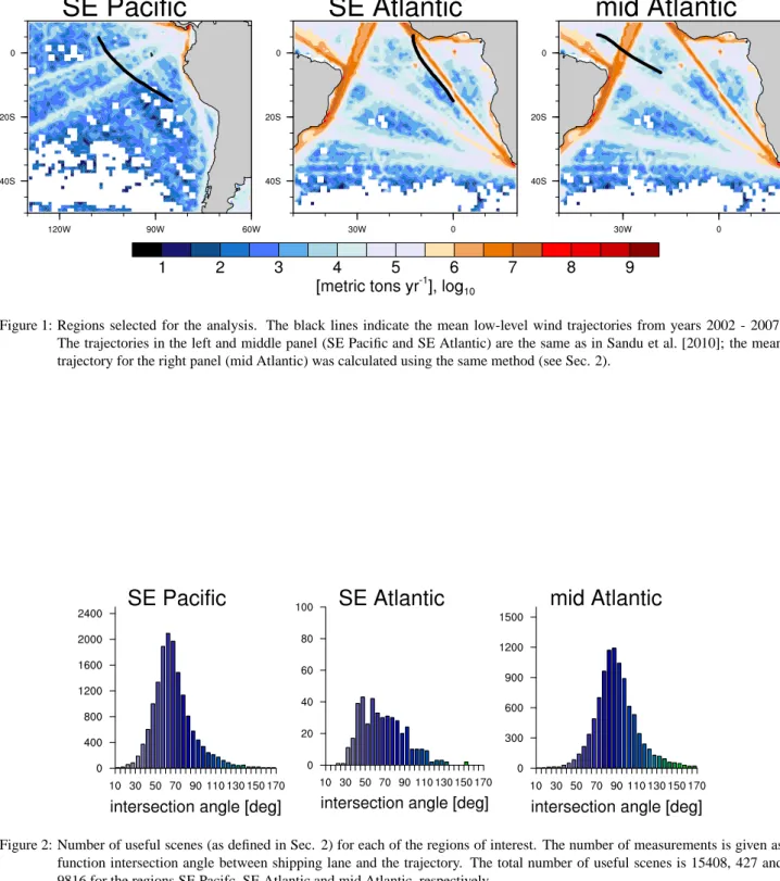
First, we select regions with large spatial contrasts in shipping emissions from visual analysis of the global shipping emission inventory presented in Endresen et al. [2005] and Endresen et al. [2007]. We select three ship-ping lanes for our analysis: (1) the shipship-ping lane from the Panama Canal to Australia, (2) the shipping lane from the southern African tip northwestwards and (3) the mid Atlantic part of the shipping lane from Europe to South America (see Fig. 1).
Figure 1: Regions selected for the analysis. The black lines indicate the mean low-level wind trajectories from years 2002 - 2007. The trajectories in the left and middle panel (SE Pacific and SE Atlantic) are the same as in Sandu et al. [2010]; the mean trajectory for the right panel (mid Atlantic) was calculated using the same method (see Sec. 2).
Figure 2: Number of useful scenes (as defined in Sec. 2) for each of the regions of interest. The number of measurements is given as function intersection angle between shipping lane and the trajectory. The total number of useful scenes is 15408, 427 and 9816 for the regions SE Pacifc, SE Atlantic and mid Atlantic, respectively.
regions from 2002 - 2007 to find scenes in which the MBL airmasses cross the respective shipping lane. By this, a separation of ”clean” (upwind) and ”pol-luted” (downwind) scenes is established. We use wind trajectories calculated with the Hybrid Single-Particle Lagrangian Integrated Trajectory Model (HYSPLIT) (http://ready.arl.noaa.gov/HYSPLIT.php) as described in Sandu et al. [2010] for the shipping lanes (1) and (2). For the analysis of shipping lane (3), we initialise wind tra-jectories from nine equally spaced points inside a grid box having upper left and lower right coordinates of (2◦S,21◦W) and (8◦S,15◦W), respectively. We calculate
the intersection point of each calculated wind trajectory with the respective shipping lane by means of linear al-gebra. This intersection point and the respective trajec-tory are classified as useful for further analysis if (1) the height of the trajectory does not exceed 500m above sea level ten hours before and ten hours after the intersection and (2) the intersection angle is 90◦±20◦. Histograms of
the amount of useful scenes as a function of intersection angles are given in Fig. 2. From this preleading analysis, we exclude the region in the southeastern Atlantic from our further analysis, because the amount of useful scenes would not ensure a sound statistical analysis.
Third, we analyse aerosol- and cloud properties along the useful trajectories. Because the trajectory model delivers hourly output of trajectory location, we are able to sam-ple for satellite data at every hour of the trajectory. We use trajectory locations ten hours before (”clean” area) and after (”polluted” area) the intersect with the shipping lane. Satellite data is analysed for every 2◦x 2◦grid box
centerd around a given trajectory point (hourly resolu-tion).
We use the publicly available MODIS Level3 collection 5 dataset for both MODIS sensors (aboard NASA’s satel-lites EOS Aqua and EOS Terra) [Platnick et al., 2003, Remer et al., 2005]. The satellite data falling into ev-ery selected 2◦x 2◦box is screened for completeness (no
missing values allowed) and presence of ice clouds (no retrieved optical thickness of ice clouds allowed). By this, the amount of data available for analysis is strongly reduced. From the screened data, we take the retrieved liquid cloud fraction (cf), cloud droplet effective radius (reff) and cloud optical depth (τ) of liquid water clouds as well as the retrieved aerosol optical depth at 0.55µm (AOD). We compute the cloud droplet number concentra-tion (CDNC) for liquid clouds from reffandτ assuming adiabaticity [Quaas et al., 2008, and references therein].
3. RESULTS
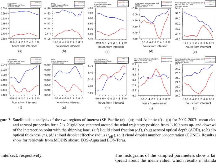
The results from the analysis of cloud- and aerosol prop-erties along shipping-lane-intersecting wind trajectories are given in Fig. 3 and Table 1.
We apply strict quality constraints to the used satellite data (see Sec. 2). This leads to a significant reduction of scenes available for the statistical analysis compared to the number of useful scenes found from the wind trajec-tory analyis (Fig. 2 and Tab. 1). Concerning data from MODIS(Terra) (MT), the number of scenes is reduced by
Table 1: Number of measurements used for cloud- and aerosol property evaluation. The number of measurements ap-plies to every hourly position in Fig. 3.
Aqua Terra Region cloud prop. AOD cloud prop. AOD SE Pacific 5910 3951 11973 7715 mid Atlantic 1010 658 2065 1554
roughly 20% and 70% for the regions SE Pacific and mid Atlantic, respectively. The number of scenes available for MODIS(Aqua) (MA) is even less because the instru-ment just started collecting data in mid 2002 and there is a data gap from January till May 2003. The number of scenes available for AOD evaluation is less than for cloud property evaluation because more 2◦x 2◦grid boxes
con-tain missing values for the AOD- than for the cloud prop-erty retrieval. The calculated mean values of cloud- and aerosol properties as a function of time to/from intersect are shown in Fig. 3.
Our analysis shows that the retrieved values of cloud-and aerosol properties do not agree well between the two MODIS instruments for most parameters. The param-eters retrieved from MT measurements are larger than those retrieved by MA except forτ and refffor the mid Atlantic. The change of the analysed parameters with time from/to intersect (TTI/TFI) is (1) generally found to be very small and (2) also seldomly consistent between the two retrievals. Furthermore, the standard deviations associated with the mean values plotted in Fig. 3 is often larger than the retrieved value itself (not shown). Concerning the results for the SE Pacific region (Figs. 3(a) - 3(e)), the only parameters where our analysis re-veals a discernible change with time is the MA-retrieved reff. Because CDNC is dependent on reff, this signal is also found there. The results show a decrease of reffat the time of intersect. reffincreases again sharply with TFI. The same holds for CDNC, just with a different sign, i.e. a sharp in- and subsequent decrease. The MT-retrieved values for reffalso show an increase with TFI. Combined with the retrievedτ, both retrievals lead to a similar slope of decreasing CDNC with TFI.
Our analysis for the mid Atlantic region shows (Figs. 3(f) - 3(j)), that the parameter being subject to the most pronounced change with TFI is the AOD retrieved by both instruments. The AOD is found to have a small but distinct maximum 4-5 hours downwind of the in-tersect. Concerning cloud microphysical properties, the MA-retrieved reffis found to subject to the largest change with time, just like in the SE Pacific region. Here, reffis found to have its maximum value at the time of intersect and it then decreases sharply with TFI. As discussed be-fore, this applies to calculated CDNC in an opposite man-ner. The MT-retrieved reffdoes not show this functional behaviour with time. Nevertheless, the MT-retrievedτ
and refflead to a systematic increase of CDNC with the complete time frame under consideration, i.e. the CDNC is lowest and highest at ten hours before and after the time
(a) (b) (c) (d) (e)
(f) (g) (h) (i) (j)
Figure 3: Satellite data analysis of the two regions of interest (SE Pacific (a) - (e); mid-Atlantic (f) - (j)) for 2002-2007: mean cloud-and aerosol properties for a 2◦x 2◦grid box centered around the wind trajectory position from 1-10 hours up- and downwind
of the intersection point with the shipping lane. (a,f) liquid cloud fraction (cf), (b,g) aerosol optical depth (AOD), (c,h) cloud optical thickness (τ), (d,i) cloud droplet effective radius (reff), (e,j) cloud droplet number concentration (CDNC). Results are
show for retrievals from MODIS aboard EOS-Aqua and EOS-Terra.
of intersect, respectively.
4. DISCUSSION AND OUTLOOK
In this paper, we presented a novel approach to sample satellite retrieved cloud- and aerosol properties to inves-tigate aerosol indirect effects stemming from shipping emissions. Satellite data are analysed along selected low-level wind trajectories which intersect shipping routes. These shipping routes are assumed to modify the MBL aerosol in such a way that their effect on cloud micro-physics can be detected downwind of the shipping lanes by statistical anlysis.
In our application of the wind trajectory analysis (see Sec. 2) we select or exclude maritime regions which are suited or not suited for the statistical analysis of aerosol- and cloud-property change due to shipping emissions. The analysis of the satellite data does not reveal the clear change in cloud- and aerosol properties from ”clean” to ”polluted” marine environments that we anticipated. The MA- and MT-retrieved parameters that we consider show very small changes with respect to time before/from inter-sect. If a systematic change is present, this change often does not comply with the conceptual picture of the first aerosol indirect effect [Twomey, 1974]. Furthermore, the computed mean values of cloud- and aerosol properties are not consistent between the MT- and MA-retrievals. These rather unsatisfying results can be due to sev-eral reasons. The most probable one is the (so far) small amount of satellite data available for the analysis.
The histograms of the sampled parameters show a large spread about the mean value, which results in standard deviations on the order of the measured value itself (not shown here).
Furthermore, the used MODIS satellite data is of rather coarse spatial (1◦x 1◦, averaged to 2◦x 2◦) resolution.
Because shipping emissions are features happening at significantly smaller scales, the use of finer resolution products might very well give clearer results. A positive side effect of this would be that the sample size would be significantly increased, thus reducing uncertainty in the statistical analysis.
Until now, we only consider one large scale meteoro-logical variable: MBL wind direction. We do not sys-tematically sample for wind speed nor do we sample for other large scale parameters like lower tropospheric sta-bility. Situations with large wind speeds lead to enhanced emission of sea-salt from the sea surface, most proba-bly burying a potential signal from ship emission influ-ence on clouds. Sampling for lower tropospheric sta-bility would enable us to separate between environments prone to the formation of large scale boundary layer liq-uid water clouds [Wood and Bretherton, 2006], which are known to be susceptible to shipping emissions [e.g. Hobbs et al., 2000].
One other reason for the results we obtained could be the choice of regions and the smallness of shipping emis-sions in general. Concerning the choice of regions, the shipping lane from Panama to Australia is probably one of the few shipping corridors where the environment can really be considered as ”pristine marine”. Nevertheless, the emissions might be too small to give a statistically
discernible effect on cloud properties in the long-term mean. The shipping emissions in the mid Atlantic region are significantly higher but aerosol advection from Africa cannot be excluded. Additionally, we have no knowl-edge about whether or not a ship is passing the shipping lane at a calculated intersection time because we only use an annual mean emission distribution. Nevertheless, the choice of a different region, e.g. the shipping corridor between Sri Lanka and Sumatra, where it has proven fea-sible to statistically derive changes in atmospheric chem-istry from satellite data [Marbach et al., 2009], may very well increase the chance of finding a systematic signal in cloud- and aerosol properties.
To further continue with this work, we will consider do-ing several thdo-ings. We plan to revise the applied method to enhance the sample size. Additionally, the sampling for other large scale meteorological variables than just MBL wind direction is most likely to enable sampling of scenes where the susceptibility of cloud microphysical properties to shipping emissions is increased. Further-more, more areas and additional satellite data will be used for the analysis. In the long run, we plan to investigate similar approaches with results from a free-run global cli-mate model (GCM) with an interactive aerosol scheme.
ACKNOWLEDGMENTS
This work is funded by the European Commission under the EU Seventh Research Framework Programme (grant agreement No 218793, MACC). We thank NASA for pro-viding free access to the MODIS data. We thank NOAA for enabling the use of the HYSPLIT model.
REFERENCES
B. A. Albrecht. Aerosols, Cloud Microphysics, and Frac-tional Cloudiness. Science, 245:1227 – 1230, 1989. E. Campmany, R. Grainger, S. Dean, and A. Sayer.
Auto-matic detection of ship tracks in ATSR-2 satellite im-agery. Atmos. Chem. Phys, 9:1899–1905, 2009. A. Devasthale, O. Kr¨uger, and H. Grassl. Impact
of ship emissions on cloud properties over coastal areas. Geophys. Res. Lett., 33(2), 2006. doi: 10.1029/2005GL024470.
P. Durkee, K. Noone, and R. Bluth. The Monterey area ship track experiment. J. Atmos. Sci., 57(16):2523– 2541, 2000.
U. Dusek, G. Frank, L. Hildebrandt, J. Curtius, J. Schnei-der, S. Walter, D. Chand, F. Drewnick, S. Hings, D. Jung, et al. Size matters more than chemistry for cloud-nucleating ability of aerosol particles. Science, 312(5778):1375–1378, 2006.
Ø. Endresen, J. Bakke, E. Sørg˚ard, T. Flat-landsmo Berglen, and P. Holmvang. Improved modelling of ship SO2 emissions–a fuel-based approach. Atmos. Environ., 39(20):3621–3628, 2005.
Ø. Endresen, E. Sørg˚ard, H. Behrens, P. Brett, and I. Isak-sen. A historical reconstruction of ships’ fuel con-sumption and emissions. J. Geophys. Res., 112(D12), 2007. doi: doi:10.1029/2006JD007630.
P. Forster, V. Ramaswamy, P. Artaxo, T. Berntsen, R. Betts, D. W. Fahey, J. Haywood, J. Lean, D. C. Lowe, G. Myhre, J. Nganga, R. Prinn, G. Raga, M. Schulz, and R. Van Dorland. Changes in At-mospheric Constituents and in Radiative Forcing. In S. Solomon, D. Qin, M. Manning, Z. Chen, M. Mar-quis, K. B. Averyt, M. Tignor, and H. L. Miller, edi-tors, Climate Change 2007: The Physical Science
Ba-sis. Contribution of Working Group I to the Fourth Assessment Report of the Intergovernmental Panel on Climate Change. Cambridge University Press,
Cam-bridge, United Kingdom and New York, NY, USA, 2007.
G. Frick and W. Hoppel. Airship measurements of ship’s exhaust plumes and their effect on marine boundary layer clouds. J. Atmos. Sci., 57(16):2625–2648, 2000. P. Hobbs, T. Garrett, R. Ferek, S. Strader, D. Hegg,
G. Frick, W. Hoppel, R. Gasparovic, L. Russell, D. Johnson, et al. Emissions from ships with respect to their effects on clouds. J. Atmos. Sci., 57(16):2570– 2590, 2000.
I. Koren, Y. Kaufman, D. Rosenfeld, L. Remer, and Y. Rudich. Aerosol invigoration and restructuring of Atlantic convective clouds. Geophys. Res. Lett., 32, 2005. doi: 10.1029/2005GL023187.
U. Lohmann and J. Feichter. Global indirect aerosol ef-fects: a review. Atmos. Chem. Phys., 5:715–737, 2005. T. Marbach, S. Beirle, U. Platt, P. Hoor, F. Wittrock, A. Richter, M. Vrekoussis, M. Grzegorski, J. P. Burrows, and T. Wagner. Satellite measurements of formaldehyde linked to shipping emissions. At-mos. Chem. Phys., 9(21):8223–8234, 2009. doi: 10.5194/acp-9-8223-2009.
A. Petzold, M. Gysel, X. Vancassel, R. Hitzenberger, H. Puxbaum, S. Vrochticky, E. Weingartner, U. Bal-tensperger, and P. Mirabel. On the effects of or-ganic matter and sulphur-containing compounds on the CCN activation of combustion particles. Atmos. Chem.
Phys., 5(12):3203, 2005.
A. Petzold, J. Hasselbach, P. Lauer, R. Baumann, K. Franke, C. Gurk, H. Schlager, and E. Weingartner. Experimental studies on particle emissions from cruis-ing ship, their characteristic properties, transformation and atmospheric lifetime in the marine boundary layer.
Atmos. Chem. Phys., 8(9):2387–2403, 2008.
S. Platnick, M. King, S. Ackerman, W. Menzel, B. Baum, J. Ri´edi, and R. Frey. The MODIS cloud products: Algorithms and examples from Terra. IEEE Trans. Geosci. Remote Sens., 41(2):459, 2003.
J. Quaas, O. Boucher, N. Bellouin, and S. Kinne. Satellite-based estimate of the direct and indirect aerosol climate forcing. J. Geophys. Res.-Atmos., 113 (D5), 2008. doi: 10.1029/2007JD008962.
L. Remer, Y. Kaufman, D. Tanre, S. Mattoo, D. Chu, J. Martins, R. Li, C. Ichoku, R. Levy, R. Kleidman, T. Eck, E. Vermote, and B. Holben. The MODIS aerosol algorithm, products, and validation. J. Atmos.
Sci., 62(4):947–973, 2005.
I. Sandu, B. Stevens, and R. Pincus. On the transitions in marine boundary layer cloudiness. Atmos. Chem.
Phys., 10(5):2377–2391, 2010. doi:
10.5194/acp-10-2377-2010.
M. Schreier, A. Kokhanovsky, V. Eyring, L. Bugliaro, H. Mannstein, B. Mayer, H. Bovensmann, and J. Bur-rows. Impact of ship emissions on the microphysi-cal, optical and radiative properties of marine stratus: a case study. Atmos. Chem. Phys., 6(12):4925–4942, 2006.
M. Schreier, H. Mannstein, V. Eyring, and H. Bovens-mann. Global ship track distribution and radiative forc-ing from 1 year of AATSR data. Geophys. Res. Lett., 34(17), 2007.
B. Stevens and G. Feingold. Untangling aerosol effects on clouds and precipitation in a buffered system.
Na-ture, 461(7264), 2009. doi: 10.1038/nature08281.
A. Teller and Z. Levin. The effects of aerosols on pre-cipitation and dimensions of subtropical clouds: a sen-sitivity study using a numerical cloud model. Atmos.
Chem. Phys., 6:67–80, 2006. doi:
10.5194/acp-6-67-2006.
S. Twomey. Pollution and the planetary albedo. Atmos.
Environ., 8:1251 – 1256, 1974.
R. Wood and C. Bretherton. On the relationship between stratiform low cloud cover and lower-tropospheric sta-bility. J. Climate, 19(24):6425–6432, 2006.