Diversification in Area-Yield Crop Insurance : The Multi Linear Additive Model

« Diversification in Area-Yield Crop Insurance

The Multi Linear Additive Model »

Geoffroy ENJOLRAS

Robert KAST

Patrick SENTIS

D

IVERSIFICATION IN

A

REA

-Y

IELD

C

ROP

I

NSURANCE

T

HE

M

ULTI

L

INEAR

A

DDITIVE

M

ODEL

Geoffroy Enjolras♦, Robert Kast♣, Patrick Sentis∗

Abstract

Diversification is the traditional way farmers use to hedge against crop yield variations. However, most insurance policies and financial contracts do not take into account this strategy in their design. In this context, we develop a of portfolio insurance model based on area-yield crop indices. This Multi-Linear Additive Model (Multi-LAM) extends previous linear approaches while it preserves their theoretical properties. We determine the conditions of use of our model and prove that it can be used despite crop yields correlations. An application to a large sample of French farms reveals the potential extent of the Multi-LAM, which significantly reduces the area-yield basis risk associated to the use of indices. We then discuss implications for crop insurance.

Keywords: Area-Yield, Crop insurance, Systemic risk, Additive model, Bootstrap.

This paper was written when Geoffroy Enjolras was a PhD student at LAMETA-INRA and CR2M.

The authors wish to thank anonymous referees for many helpful comments on earlier drafts of this paper. All remaining errors are the responsibility of the authors. An earlier version of the paper was presented at the 36th Seminar of the European Group of Risk and Insurance Economists (EGRIE), Bergen, Norway, September 21-23, 2009.

♦ _{Université de la Méditerranée Aix-Marseille 2, Faculté des Sciences Economiques et de Gestion, CRET-LOG,} 14 avenue Jules Ferry, 13621 Aix-en-Provence Cedex, France.

Corresponding author: [email protected]

♣ _{Université Montpellier 1, CNRS, LAMETA - INRA, 2 place Pierre Viala, 34060 Montpellier Cedex 1, France.} [email protected]

∗ _{Université Montpellier 1, CR2M, ISEM, GSCM Montpellier Business School, Avenue de la Mer, 34054} Montpellier Cedex 1, France. [email protected]

1. Introduction

Recent research proves that farms have been using for thousands of years crop diversification (Colledge et al., 2005). This behavior was mainly motivated by a desire to protect communities against climatic hazards. In fact, agriculture suffers from a higher vulnerability compared to other sectors of the economy as it depends directly on weather. In modern area, the agricultural sector has always been favored because of its strategic importance.

Thus, diversification mechanisms have been progressively complemented – but not completely replaced – by financial instruments. In developed countries, insurance systems against natural catastrophes are now widely developed and they take different aspects involving both the governments and the insurers. The governments’ subsidies, associated to the efforts made on risk modeling improvement, encouraged the development of an active market. Leading instruments are Multi-Peril Crop Insurance, Group Risk (Income) Plan and Catastrophe Insurance (e.g. the Supplemental Revenue Assistance Program in the USA).

The farmer’s choice between these different products depends on the scope of coverage. For instance, area yield insurance implies to focus the coverage on the systematic part of a given catastrophic risk, which is common to all insured in a given region. In counterpart, the individual part of the catastrophic risk is neglected as it mainly depends on each farmer’s behavior towards the risk. This fact may explain why insurance products are not subscribed by farmers unless they are highly subsidized. In this context of incomplete markets, there is a need for new theoretical models whose aim is to improve the efficiency of the coverage. The design of the contracts should take into account both the individual characteristic of the farm and the climatic risk which affects its localization.

A first major challenge consists in identifying the two components of a catastrophic risk. We refer to the “regressability” assumption, as stated by Benninga et al. (1984). This method consists in orthogonally projecting a producer’s individual yield onto an area yield. It is then possible to determine the sensitivity of the producer’s individual yield to the systematic factors that affect the area yield (Miranda, 1991). This model is commonly defined as the Linear Additive Model (LAM). Aggregated indexes allow to capture the consequences of a natural catastrophe affecting a given area. Moreover, regional yields come from an

of the yields explained by a regional index is considered as a systematic risk while the residual component of the model is assumed to be the idiosyncratic part of the risk.

A second challenge concerns the use of adapted financial indices. In particular, the size of the area needs to be debated in order to find a compromise between the basis risk and information asymmetries. The choice to focus at an individual or a regional scale has been widely debated. Barnett et al. (2005) proved that reasoning at an area level rather than at an individual level presents several advantages in terms of efficiency. When reasoning at an area level, regional indices should be preferred to national ones (Mahul and Vermersch, 2000). A recent French report from the Ministry of Agriculture (Mortemousque, 2007) reveals that indices are only defined with respect to climate. They usually refer to an administrative basis that may be adjusted, depending on climate diversity. The indexes are usually defined in quintals per hectare or bushels per acre. Contrary to a monetary index, this measurement is reasonably objective because it is directly observable. Moreover, prices may vary over a given year, which could increase the insurers’ exposure. For this reason, in most contracts prices are set prior to subscription and in accordance with their evolution in previous years.

A third challenge addresses the problem of the design of the optimal coverage policy for a “crop portfolio”. Several analyses have already been devoted to area yield crop insurance but they only consider coverage for one crop or even one kind of risk (see e.g. Miranda, 1991, Mahul and Vermersch, 2000 and Deng et al., 2007). As a result, the replication of this portfolio usually takes the form of a juxtaposition of separate contracts for each crop or the implementation of insurance at the farm scale. None of these techniques correctly takes diversification into account. Faced to major climatic risks, a farmer is naturally induced to reduce his exposition by selecting activities or groups of activities whose yields are less correlated. Optimal insurance should consider this effort, which should reduce overall risk. In regards to the three challenges exposed above, it appears necessary to adapt the existing instruments. Taking into account diversification implies to extend the usual LAM model to a crop portfolio. The main goal of this article is to define a Multi Linear Additive Model (Multi-LAM). The Multi-LAM is designed at the farm’s scale, which allows considering the risk structure of the farm, i.e. individual risks in addition to systematic ones. Therefore, an additional challenge consists in integrating the impact of crop yield correlation in the analysis.

It represents a necessary condition for the validity of the model as some indices may be redundant.

Estimating the model in practice also requires a large number of historic records for each crop and each farm. Usually, databases are rather limited. To overcome this constraint which has been noticed but never really solved by literature (see e.g. Barnett et al., 2005), we apply the bootstrap technique on available data. This technique has been widely implemented, especially in finance when annual data are used (Ruiz and Pascual, 2002). This allows testing the efficiency of the Multi-LAM with a larger sample.

In the second section of this article, we recall the Linear Additive Model (LAM) and explore the ways to extend it to a crop portfolio. In the third section, we define the Multi-LAM and develop its main properties. In the fourth section, we present a methodology and the data used for evaluating the performances of the Multi-LAM. In the fifth section, we expose our empirical results and their implications for crop insurance. Finally, in the sixth section, we discuss the potential applications of the Multi-LAM for crop insurance hedging.

2. The Linear Additive Model and its extensions

The aim of the Linear Additive Model (LAM) is to describe a relationship between individual yields and the mean yield in a given area and for a given crop. In this section, we present successively the LAM and its potential extensions when considering the full crop portfolio of a farm.

The LAM considers only one crop yield for a given farmer i. It can be written as follows:

( )

(

( )

)

i i i i

y% =E y% +β y E y%− % +ε%

Where yi is the individual yield, y is the area yield, β_i is the sensitivity of the individual crop

yield to the movements of the crop area yield and εi is the residual of the model. The tilde

The simplicity of its formulation has made the LAM largely used in agricultural economics since Miranda (1991). However, the theoretical foundations for the LAM were formalized for the first time by Rawaswami and Roe in 2004.

Following this rich literature, we propose to extend the LAM to a crop portfolio by exploring several paths which preserve the use of indices and the linearity of the model:

- The first method consists in estimating standard LAM models for each crop. Starting from a separate estimation of the beta coefficients, the farmer’s crop portfolio is replicated ex post. We propose to call it “Additive LAM”.

- The second method consists in estimating a unique LAM for the whole farm. It involves computing an aggregated area-index based on the composition of the crop portfolio of the farm. We name it “Farm LAM”.

- The third method is the Multi-LAM, as we propose to name it. It consists in estimating a single model with a number of area yield indexes equal to the number of crops in the farmer’s portfolio. The purpose is to provide more reliable results through better adjustment of the data.

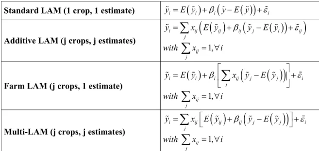
The mathematical formulations of these three strategies are detailed in Table 1. Table 1. Strategies for a LAM transposed to a crop portfolio.

The Additive LAM and the Farm LAM are trivial extensions of the Linear Additive Model. However, estimating a Multi-LAM requires to study its main properties. We therefore focus our analysis on this model.

3. The Multi-Linear Additive Model

Generalizing the LAM to a Multi-LAM preserves the linear structure of the model, which allows to determine with precision some essential properties for its validity. In particular, we take care to verify and extend the theoretical results of the LAM (Rawaswami and Roe, 2004) when there are many crops.

3.1 Formalization of the Multi-LAM

Designed at the farm-level, the Multi-LAM takes the following form:

(1) _{i ij}

( )

_{ij ij ij}

(

_j

( )

_j

)

_i

j j

y =

∑

x E y +

∑

x β y −E y +ε

Where yi is the global yield of farm i, yj is the area yield of crop j. We note xij as the control variable, which defines the proportions of each crop in the farmer’s portfolio. By definition,

1 ij j

x =

∑

for each farm. εi is a random variable, which is not correlated with the area yield of the different crops.

Equation (1) breaks down individual yield variations of the different crops i ij

( )

ij j

y −

∑

x E y

into two components: a systematic component ij ij

(

j

( )

j

)

j

x β y −E y

∑

whose elements are

perfectly correlated with the area yields and an individual component εi which is not correlated with these individual yields.

In accordance with Rawaswami and Roe (2004), we choose to use a structural model which defines the individual yield yij for each crop j of farm i as a function f of an individual component eij and a systematic component θj.

This structural form is written as follows: y_ij = f e_ij

(

_ij,θ_j

)

At the farm-level, we can then define: i ij ij ij ij

(

ij, j

)

j j

y =

∑

x y =

∑

x f e θ

In practice, function f can take several forms. We present some specifications cited by Ramaswami and Roe (2004) and their extension to a crop portfolio in Table 2.

Table 2. Yield specifications generalized to a multi-crop analysis

Starting from these specifications, we must answer three main questions: Which properties must the LAM model satisfy? Conversely, which classes of models imply a Multi-LAM? What is the validity of the Multi-LAM when yield aggregation is performed at a small scale?

3.2 An example of structural model for the Multi-LAM: Multiplicative Risks and Additive Components (MRAC)

The aim of this sub-section is to determine the main properties that a Multi-LAM model must satisfy. Starting from the general specifications exposed in Table 2, we study a particular class of model called “Multiplicative Risks and Additive Components” (MRAC). The conclusion of this analysis will yield a general structural model.

According to literature, the MRAC model, which adds multiplicative risks, is realistic for crop yield variations (see e.g. Mahul, 1998, and Ramaswami and Roe, 2004). In this case, the individual mean yield is a stochastic function of inputs controlled by the producer.

Let us consider an area with N farmers. Following the specification of the MRAC in Table 2, we define the yield of crop j for farmer i with the following equation:

Where η_ij is a random variable, which captures the different risks associated with the farmer’s crop portfolio.

Equation (2) is a standard specification where risks are multiplicative to mean yields. With respect to the form of the Multi-LAM defined in (1), the risk is captured through a random variable given by:

(3) η_ij =α_{j ij}e +γ θ_{j j}

Where eij is a shock specific to crop j and to farm i and θj is a shock common to all producers who cultivate crop j. By definition, the first shock is individual while the second is systematic. We assume individual and systematic risks satisfy the following properties:

- E

( )

θ_j = ∀1, j - E e

( )

_ij = ∀1, ,i j - Cov e

(

_ij,θ_j

)

= ∀0, ,i j - Cov e e

(

_ij, _kj

)

= ∀ ≠0, i k j,

- α_j+γ_j = ∀1, j (Unit-mean constraint)

According to (2) and (3), these properties imply that:

(4) _{i ij}

( )(

_{ij j ij j j}

)

j

y =

∑

x E y α e +γ θ

Proposition 1: (a) In the MRAC model described by equations (2) to (4), the relationships between individual and area yields are in line with a Multi-LAM. (b) The parameters of the Multi-LAM are linked to the structural model in the following manner:

( )

( )

ij ij j E y E y β = and

( )(

1

)

i j ij j ij j x E y e ε =

∑

α −

The implications for each part of Proposition 1 are as follows:

(a) For all crops cultivated by an individual producer, the beta parameter is equal to the ratio between individual mean yield and mean regional yield, which implies:

1, ij ij i j ω β = ∀

∑

1

(b) The error term is heteroskedastic:

( )

2

( )

2 2 2

i ij ij j ij

j

Var ε =

∑

x E y α e

Under a MRAC formulation, the general model does not specify the functional forms of either the input or the yield. Nor does it specify the density of probability of individual and systematic risks. A similar reasoning can be applied to other specifications, e.g. additive risks and additive components (ARAC).

3.3 A general structural model for the Multi-LAM

The purpose of this section is to determine the class of models which imply a Multi-LAM. We does so by looking for model characteristics that do not imply a Multi-LAM.

The structural form of production of crop j in farm i is given by the following equation:

(5) y_ij = f_ij

(

θ_j, ,e E y_ij

( )

_ij

)

≡ f_ij

(

θ_j,e_ij

)

where θ_j and e_ij are respectively the random realizations of systematic and individual shocks.

( )

ij

E y is a vector of realized yields, which implies that we can omit it from our notations in the next steps.

1 _{Where ω}

Proposition 2: If the relationship between individual and area yields is described by a Multi-LAM as in (1), then the structural model necessarily satisfies: (a)

( )

( )

ij ij ij ij ij ij j

j j

y =

∑

x h e +

∑

x g θ , where hij and gij are functions which characterize respectively the impact of individual and systematic shocks on individual yields. (b) ∀i, there is a function l(θ) and a parameter λi such that: g_ij

( )

θ_j =λ θ_ijl

( )

_j +c_ij,where cij is a constant of integration.

Proof is detailed in Appendix 2.

Proposition 2 specifies the class of structural models implied by the Multi-LAM. We notice that the components of the risk are additive on the production level. As there are no constraints on functions h and g, the way a given risk affect the production do not need to be specified.

By this stage, the main question is to discover whether each class of structural model identified in Proposition 2 implies a Multi-LAM. Proposition 3 confirms this assumption provided the aggregation at the regional level is sufficiently large.

Proposition 3: Structural model (5) implies a multi-LAM if: (a) The weighted average of the risks can be replaced by the average of a large population. (b) The structural model satisfies: (6) _{i ij ij ij ij j}

( )

_{j ij ij}

( )

_ij

j j j

y =

∑

x a +

∑

x b l θ +

∑

x h e , where l_j

( )

θ_j and h e are monotonic _ij

( )

_ij functions and aij and bij are parameters which can vary with i and j.

Proof is detailed in Appendix 3.

It clearly appears that εi is a random variable with a mean equal to zero and which is not correlated with the different area yields. The last equation of the demonstration gives the relationship between the parameters of the structural model and the parameters of the Multi-LAM.

Proposition 4: The parameters of the general structural model, which is equivalent to a Multi-LAM, satisfy (a) ij

ij j b b β = and (b) _{i ij ij}

( )

_ij

(

_ij

( )

_ij

)

j x h e E h e ε =

∑

⎡_⎣ − ⎤_⎦

Part (a) means that yield sensitivity of crop j from farm i, compared to the area yield of crop j, is equal to the sensitivity of the yield of crop j from farm i to a systematic shock, when compared to the sensitivity of area yield to a systematic shock.

Assuming the independence of the h e_ij

( )

_ij terms, part (b) implies that:

( )

2

( )

i ij ij ij

j

Var ε =

∑

x Var h e⎡_⎣ ⎤_⎦

Using Proposition 4, we can specify theβ_ij coefficients for the usual specifications described in Table 2.

Let us focus first on the MRAC model examined earlier: _{i ij}

( )

_{ij ij j} j y =

∑

x E y ⎡_⎣αe +γθ ⎤_⎦ Therefore, ∀k l, _j

( ) ( )

θ_j =E y_ij γ θ_{j j} ,

( )

( )

ij ij kj E y b E y = and h e_ij

( ) ( )

_ij =E y_ij α_{j ij}e

A particular case of the structural model is obtained with the following individual yield:

( ) ( )

j ij ij j j ij ij j y =

∑

x b l⎡_⎣ θ +h e ⎤_⎦ Here,

( )

( )

j , j kj E y b j E y

= ∀ and using Proposition 3, we find that:

( )

( )

ij ij j E y E y β =

The ARAC model _{i ij}

( )

_{ij ij j} j

y =

∑

x E y⎡_⎣ + +e θ ⎤_⎦ is a particular and trivial case of the structural model with additive risks. Here, b_ij =1 implies that b_j =1 and β_ij = ∀1, ,i j.

Yield heterogeneity associated to the different crops has no impact on the yield of the farm.

The JPAC model _{i ij}

( )

_{ij ij}

(

_{ij j}

)

j

y =

∑

x E y⎡_⎣ +σ e +θ ⎤_⎦ is also a particular case of the structural model. Here, l_j

( )

θ_j =θ_j and b_ij =σ_ij implies that b_j =σ_j, with _{j ij ij ij} ij

i j

σ

σ ω σ β

σ

=

∑

→ = .

Finally, the MRMC model does not satisfy the specifications of the Multi-LAM as there are no linear components.

3.4 Validity of the Multi-LAM when aggregating on small samples

Proposition 1 defines the Multi-LAM as a consequence of the additive interaction between individual and systematic risks. However, this condition is necessary but not sufficient for the validity of this model. Moreover, Propositions 3 and 4 assume a large area defined by a wide sample. The main question is to discuss the validity of the Multi-LAM when the area is defined by a small number of farms. In practice, the definition of the area scale is essential for the implementation of the Multi-LAM. This is the aim of Proposition 5.

Proposition 5: Small aggregation leads to inconsistent econometric estimates but the other properties and results of the Multi-LAM still remain valid.

Proof is detailed in Appendix 4.

Despite the econometric issue, the properties and results of the Multi-LAM exposed above still remain valid. We also found that the main properties of the Linear Additive Model were preserved when it was extended to a crop portfolio.

Small aggregation remains a major challenge for the design of the Multi-LAM. In practice, the definition of each area must correspond to equilibrium between precision and representation: it must not be too large for the quality of the adjustment, but needs to be enough significant so that no farm in the area can be of a predominant size. Then we can test the validity of the Multi-LAM.

4. Testing the validity of the Multi-LAM: Methodology and database 4.1 Main assumptions

Using the definition given of the Multi-LAM, we can assume that this formulation provides a better adjustment than the addition of LAM or a Farm LAM. In the first case, estimating the parameters of a Multi-LAM directly takes into account the composition of the crop portfolio in the farm considered, while it is exogenous with an additive LAM. This issue is taken into account with a Farm LAM, but such modeling (1 beta) probably does not fit well with the diversity of the portfolio (j crops).

Moreover, the theoretical properties of the Multi-LAM may be valid if, and only if, certain conditions are satisfied. The first refers to the size of the area which is used as a reference (see Proposition 5). We shall also take into account a standard econometric argument: for the validity of the model, crop yields introduced into the Multi-LAM must not be correlated. This condition may appear restrictive but it can be overcome by determining ex-ante significant classes of crops whose yields are not correlated. In practice, one crop is usually used as a reference, e.g. wheat for cereals, which is quite restrictive.

We measure the efficiency of each coverage strategy considering the residual - or basis - risk. If the Multi-LAM is more efficient, then the variance in the basis risk with this strategy should be significantly lower than using an Additive LAM or a Farm LAM (Elton and Gruber, 1997). In order to measure this efficiency, we use exactly the same data when estimating the results for all the strategies. In each case, the distribution of the residuals is compared by performing a Mann-Whitney test.

4.2 The data from FADN

The study uses a survey of French farmers who are members of the Farm Accountancy Data Network (FADN). Data are accounted for each year from a representative sample of farms of Northern France2, whose size can be considered to be commercial. We selected a set of farms whose accounting data were available from 1990 to 2006 and which cultivated at least two crops, i.e. 1,732 farms. The regional data come from the AGRESTE database, which contains aggregate indicators for each crop and for each administrative region. In line with Mahul et al. (2000), this eliminated the need to compute yield expectations with our sample. Moreover, it prevented the problem of small aggregations.

For each region, we computed the correlation coefficients between crop yields using available historical data. This allowed us defining classes of crops.

Table 3. Correlation coefficients between wheat, sugar beet and other crops in Northern France Table 3 shows that in Northern France the yields of wheat, barley, pea and rapeseed are closely correlated. Sugar beet yield is also correlated with those of maize and sunflower. Therefore, in these regions, we could select at least two crops of reference: wheat and sugar beet. This kind of “grouping” is mainly used in practice when, for sake of simplicity, wheat yield variations are considered as the unique reference for all crops.

In order to estimate the Multi-Linear Additive Model, we needed to identify different groups of farms according to their diversification level:

- Group 1: 402 farms (23%) which only cultivated uncorrelated crops. In this case, the Multi-LAM can be directly estimated.

- Group 2: 875 farms (50%) which cultivated both correlated and uncorrelated crops but it was possible to identify crops of reference as stated above. Therefore the Multi-LAM could be estimated.

- Group 3: 455 farms (27%) which cultivated only correlated crops. For these farms, a single LAM is enough and a crop of reference must be chosen. This choice can be done regarding the most cultivated crop.

According to our sample, 73% of the farms are quite diversified (Groups 1 and 2). For these farms, the Multi-LAM model can be estimated provided some adjustments when it is necessary to group crops.

4.3 Using the bootstrap technique

In order to verify if our main assumption is satisfied, we need to estimate the econometric models for Additive LAM, Farm LAM and Multi-LAM. As our dataset is available at most for 12 years, we decided to resample it with the purpose of estimating linear regressions. In practice and for samples of farm coming from Group 1 and Group 2, we bootstrap the original data. Originally proposed by Efron (1979), this is a computation-intensive method for estimating the distribution of a test statistic or a parameter estimator by resampling the data3_.

Although it retains correlation, the bootstrap is particularly useful in cases where the asymptotic distribution is difficult to obtain, or simply unknown. In addition, this method often generates higher-order accurate estimates of the distribution which improve upon the usual asymptotic approximations (Chou and Zhou, 2006). Because of these advantages, it is not surprising to find applications of the bootstrap method in finance, in particular for estimating regression coefficients (see e.g. Balduzzi and Robotti, 2005). Of the different methodologies, the one developed by Hall (1994) provides the most relevant and accurate estimates, as their standard deviation is reduced.

In order to perform a direct comparison between the different theoretical approaches, we use each bootstrap resample to estimate the different models (Additive LAM, Farm LAM and Multi-LAM). Then we look at the validity of these three different approaches through the residuals in the models4. The residuals help determining the “individual risk” also known as “area yield basis risk” because they are not explained by area yield indices. As stated before, the variance of this risk should be lower using a Multi-LAM approach.

3 _{For each farm, we start from available data and create 1,000 new samples, each one containing}

1,000 observations. These additional datasets are then used to estimate precisely regression coefficients and residuals for Additive LAM, Farm LAM and Multi-LAM.

4 _{Multi-LAM and Farm LAM directly provides the regression residuals while it is necessary to compute them for}

Additive LAM. In that case, we had to subtract the estimated values from the original values, with respect to the weight of each crop in the considered farms.

5. Empirical results

We chose to test in practice the validity of the Multi-LAM considering two samples coming from Group 1 (uncorrelated crops) and Group 2 (regrouped crops).

5.1 Estimation and validity tests for Group 1

Farms that belong to Group 1 cultivated only crops whose yields are not correlated. Therefore we could consider they are diversified without using insurance. Among these farms, we chose to study those for which crop diversification was not efficient: their yield variation at the farm-scale was higher than the mean of farms that belong to Group 1. This represented one fourth of the farms with uncorrelated yields, i.e. 105 farms. Among these farms, 68 cultivated only wheat and sugar beet, which allowed us to define a quite homogenous sample.

When performing the regression for all our models, we noticed that distribution of the beta coefficients changed between the different models. The coefficients associated with the Additive LAM were estimated separately for each crop. In this particular case, we found a result conform to the literature, i.e. a bell-shaped distribution of beta centered on unity. For the Multi-LAM, the distribution of beta coefficients did not have these properties, probably because of the adjustment between the two crop yields.

The most important result was provided when eliciting the area yield basis risk. We estimated (Farm LAM, Multi-LAM) or computed (Additive LAM) the basis risk for each bootstrapped sample of a given farm. In that case, measurement of the variance was more accurate and precise. A sample of the computations for ten farms is given in Appendix 5. For each farm, we provided summary indicators: its normal (average) yield and its yield variance. For each method, we detailed the values of the coefficients and both the systematic and yield basis risk. These synthetic indicators have already been used to measure the quality of adjustment with various methods (Mahul and Vermersch, 2002). The yield basis risk is defined as the percentage of variance of the yield basis risk in variance of the individual yield risk. Conversely, systematic risk is the percentage of variance of the systematic component in variance of the individual yield risk.

A sample of the computations is exposed in Appendix 5. Let us consider for instance the first farm of our sample. Combining its wheat and sugar beet production with respect to their proportion in the farm, the mean yield of this farm is equal to 241.87 quintals per are. Its yield variance is equal to 11.77 squared quintals per are. The estimation of a LAM at the farm’s scale provides a bootstrapped beta coefficient equal to 0.44 and a yield basis risk up to 33.45%. If we estimate separate LAM for each crop, we get an Additive LAM with two bootstrapped betas: β = 0.69 is associated with wheat and β = 1.13 is associated with sugar beet. The value of the area yield basis risk is equal to 37.22%, which is higher than for a Farm LAM. With a Multi-LAM, β = 2.67 is associated with wheat and β = 0.24 is associated with sugar beet. The yield basis risk decreases to 25.93%, i.e. -30.33% compared to the Additive LAM and -22.48% compared to the Farm LAM.

For the whole sample, we clearly noticed that the yield basis risk was lower when performing a Multi-LAM compared to the other strategies: Farm LAM or Additive LAM. In 59 cases out of 68, the variance of the area-basis risk was lower with a Multi-LAM than with an Additive LAM and in 55 cases out of 68, it was lower than with a Farm LAM. An illustration of this reduction is provided in Appendix 6 for the ten first farms of the sample.

Table 4. Summary statistics and Mann-Whitney test

between distributions of variance in the yield basis risk for Group 1.

Table 4 shows that Mann-Whitney tests performed between the Multi-LAM and respectively with the Additive LAM and the Farm LAM confirm the difference in distributions of variances in the area yield basis risk. The same test between the Farm LAM and the Additive LAM does not show a significant difference between the two distributions. We are then able to conclude that the explanatory power of the Additive LAM and Farm LAM are reasonably equivalent in this case. In this example, the Multi-LAM thus appears to be a good way to reduce the basis risk associated with an area crop-yield index.

5.2 Estimation and validity tests for Group 2

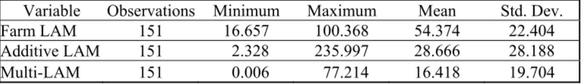
Farms that belong to Group 2 cultivate crops whose yields are correlated. However, it is possible to find crops of reference so that the Multi-LAM applies. Starting from our 875 farms, we made a random sampling with the aim of creating a new dataset of 151 farms. For each farm, we made groupings, mainly on wheat and sugar beet. Implicitly we assumed the yield of “grouped” crops varied more or less the same than “original” crops. In practice, we added the areas of grouped crops, which redefined and reduced the number of control variables xij. Each xij is now defined as the proportions of each class of crop in the farmer’s portfolio, which is the main difference compared to previous case.

Therefore, we can focus directly on the distributions of variance in the yield basis risk. Test for Group 2 present similar results than for Group 1, i.e. a better performance of the Multi-LAM compared to other strategies: Farm Multi-LAM or Additive Multi-LAM. In 110 cases out of 151, the variance of the basis risk was lower with a Multi-LAM than with an Additive LAM and in 130 cases out of 151, it was lower than with a Farm LAM.

Table 5. Summary statistics and Mann-Whitney test

between distributions of variance in the yield basis risk for Group 2.

Table 5 shows that Mann-Whitney tests performed between the Multi-LAM and respectively with the Additive LAM and the Farm LAM confirm the difference in distributions of variances in the yield basis risk. In our example, the Multi-LAM thus appears to be a good way of reducing the basis risk associated with an area crop-yield index, even if crops are regrouped. The same Mann-Whitney test between the Farm LAM and the Additive LAM exhibits a significant difference in favor of the Additive LAM. In this case, the explanatory power of the Additive LAM is higher than the one of the Farm LAM, which implies that the use of many instruments is better than a single - but integrated - instrument. The size of the sample may explain this additional result compared to Group 1.

6. Perspectives for insurance policies

The estimated parameters of the Multi-LAM offer many implications for crop insurance regarding the traditional uses of the beta coefficients in finance. In our model, these parameters estimate the sensibility of an individual yield to an area yield while taking into account the crop portfolio structure. As observed by Ramaswami et al. (2004), there exists an analogy between the formulations of the Linear Additive Model (LAM) and of the Sharpe's single-index model. However, Sharpe’s model is used for pricing which is not the aim of the LAM. Similarly, when extending the LAM to a Multi-LAM, one can find similarities between this new formulation and a multifactor model (Ross, 1976).

Previous studies emphasized the equivalence between beta coefficients and hedge positions with financial policies (see for instance Miranda, 1991, Smith et al., 1994, Mahul, 1999, Chambers and Quiggin, 2002, Rejesus et al., 2006 or Deng et al., 2007). This comes from the financial signification of the beta coefficient, which is the sensitivity of the producer’s yield to the movements of the area yields of crop j. In fact, the literature focused on models with a single variable and a single beta. In a mean-variance framework, Miranda (1991) found that optimal farmer’s behavior is to take out an insurance contract with a coverage level that equals his positive individual beta. Mahul and Vermersch (2000) derived hedge ratios from their estimated beta. Then they proposed a set of financial contracts including futures and options in order to hedge crop risk.

However, these studies are constrained to the use of a single beta or a set of beta estimated separately for each crop. The Multi-LAM takes into account farm diversification when differentiating the individual and systematic components of a given risk. It thus reinforces the results of Barnett et al. (2005) in two ways:

- The specific risk – or area yield basis risk – is the result of coverage inefficiency. We proved it was significantly reduced with a Multi-LAM, either with uncorrelated crops or groups of uncorrelated crops. Moreover, this kind of risk was independent between the different farmers in a given area because it mainly depended on the structure of the crop portfolio. We thus guess that it can be hedged more easily with private insurance. Therefore, standard policies may be used, or even participating policies (Enjolras and Kast, 2008), in order to provide a fully integrated coverage.

- In our two examples, the relative importance of the systematic risk was higher estimating a Multi-LAM. Then, the use of the beta coefficients estimated with a Multi-LAM function may be more accurate than the coefficients estimated with single LAMs. Moreover, hedging with existing instruments should be facilitated. This should also make crop risk insurable on financial markets.

These interpretations are related to the linear assumption of the Multi-LAM. Its formulation helps to provide precise theoretical propositions and associated results. It is also a way to perform direct comparisons with existing approaches. Moreover, the strong statistical significance of the Multi-LAM shows the relevancy of this choice. The use of nonlinear models is being developed in literature (see e.g. Cabrera et al., 2007) and it offers some other promising results. It seems that this approach could be an extension of our work. In particular, its implementation should take into account that diversification contributes to smooth yield variations of the crop portfolio.

7. Conclusion

This article contributed to restore the importance of diversification in crop insurance. Extending previous studies, we proved that use of a linear model is compatible with many specifications of crop yields already stated. We also showed that considering ex-ante the diversity of a farm crop portfolio could lead to a significant reduction of the individual component of the risk, which is neglected when subscribing only financial policies.

Estimating in practice the Multi-LAM, which is an econometric model, requires fulfilling some conditions: for instance the definition of homogeneous areas, i.e. with the same climate and with a sufficient number of farms, so that the area yield is correctly correlated with the individual yields. It is also necessary to define crops of reference in order to avoid correlations effects in the model.

Our database at the French level showed that most farms which cultivate at least two crops are potentially concerned by the Multi-LAM. This result opens up numerous perspectives for a commercial application. With a set of adjusted betas, we can presume that the existing models with a single crop can be adapted in order to design optimal hedging strategies, even with existing instruments. Furthermore, the bootstrap technique makes it possible to overcome the lack of historical data. For this reason, this new parameterization of financial instruments could be adapted to the pricing and the extension of the crop insurance market.

References

Balduzzi P. and Robotti C. (2005), “Mimicking Portfolios, Economic Risk Premia, and Tests of Multi-beta Models". Working paper series, Federal Reserve Bank of Atlanta, 2005-4. Barnett, B. J., Black J. R., Hu Y. and Skees J.R. (2005). “Is Area Yield Insurance Competitive with Farm Yield Insurance?”. Journal of Agricultural and Resource Economics, 30: 285-301. Benninga S., Eldor R. and Zilcha I. (1984). “The optimal hedge ratio in unbiased futures markets”. Journal of Futures Markets, 4(2): 155-161.

Cabrera V.E., Solis D. and Letson D. (2007). “Optimal crop-insurance strategies under climate variability: Contrasting insurer and farmer interests”, Proceedings of the American Agricultural Economics Association Annual Meeting, Portland, July 29-August 1, 2007. Chambers R. G. and Quiggin J. (2002). “Optimal producer behavior in the presence of area-yield crop insurance”. American Journal of Agricultural Economics, 84: 320–34.

Chou P.H. and Zhou G. (2006). “Using Bootstrap to Test Portfolio Efficiency”. Annals of Economics and Finance, 7: 217–249.

Colledge S., Conolly J. and Shennan S. (2005). “The evolution of early Neolithic farming from SW Asian origins to NW European limits”. European Journal of Archaeology, 8(2): 137-156.

Deng X., Barnett B.J. and Vedenov D.V. (2007). "Is There a Viable Market for Area-Based Crop Insurance?". American Journal of Agricultural Economics, 89(2): 508-519.

Efron B. (1979). "Bootstrap Methods: Another Look at the Jackknife". The Annals of Statistics, 7 (1): 1–26.

Elton E.J. and Gruber M.J. (1997). "Modern portfolio theory, 1950 to date". Journal of Banking and Finance, 21: 1743-1759.

Enjolras G. and Kast R. (2008). “Using Participating and Financial Contracts to Insure Catastrophe Risk: Implications for Crop Risk Management”. Lameta Working Paper, 2008-1. Hall P. (1994). “Methodology and Theory for the Bootstrap, Chapter 39” in Engle R. F. and

Just R.E. and Pope R.D. (1979). “Production Function Estimation and Related Risk Considerations”, American Journal of Agricultural Economics, 61: 277-284.

Kosowski R, Timmermann A, Wermers R and White H (2006). “Can mutual fund "stars" really pick stocks? New evidence from a bootstrap analysis”. Journal of Finance, 61: 2551-2595.

Mahul O. (1999), “Optimum Area Yield Crop Insurance”. American Journal of Agricultural Economics, 81(1): 75–82.

Mahul O. and Vermersch D. (2000). “Hedging crop risk with yield insurance futures and Options”. European Review of Agricultural Economics, 27(2): 109-126.

Malliaropulos D. (1996). “Are long-horizon stock returns predictable? A bootstrap analysis”. Journal of Business Finance and Accounting, 23: 93–106.

Miranda M.J. (1991). “Area-Yield Crop Insurance Reconsidered”. American Journal of Agricultural Economics, 73: 233-42.

Mortemousque D. (2007). “Une nouvelle étape pour la diffusion de l'assurance récolte”. Ministère de l'agriculture et de la pêche, Paris, 50 pp.

Nawalkha S. (1997). "A Multibeta Representation Theorem for Linear Asset Pricing Theories". Journal of Financial Economics, 46(3): 357-381.

Peters S.C. and Freedman D.A. (1984). “Some Notes on the Bootstrap in Regression Problems”, Journal of Business & Economic Statistics, 2(4): 406-409.

Ramaswami B. and Roe T.L. (2004). “Aggregation in Area-Yield Crop Insurance: The Linear Additive Model”. American Journal of Agricultural Economics, 86(2): 420-431.

Rejesus R.M., Coble K.H., Knight T. and Yufei J. (2006). "Developing Experience-Based Premium Rate Discounts in Crop Insurance". American Journal of Agricultural Economics, 88(2): 409-419.

Ross S.A. (1976). "The arbitrage theory of capital asset pricing”. Journal of Economic Theory, 13(3): 341-360.

Ruiz, E. and Pascual L. (2002). “Bootstrapping Financial Time Series”. Journal of Economic Surveys, 16(3): 271-300.

Shanken J. (1985). “Multi-beta CAPM or equilibrium APT?: A reply”. Journal of Finance, 40: 1189-1196.

Smith V.H., Chouinard H.H. and Baquet A.E. (1994). “Almost Ideal Area Yield Crop Insurance Contracts”. Agricultural and Resource Economic Review, 23:75-83.

Appendix 1. Proof of Proposition 1 Extending (4), the area yield of crop j can be written as:

(A1) _{j ij ij j j ij}

( )

_{ij j ij}

( )

_{ij ij}

i i i

y = ω y =γ θ _⎜⎛ ω E y _⎟⎞+α ⎛_⎜ ω E y e ⎞_⎟

⎝ ⎠ ⎝ ⎠

∑

∑

∑

Where ωij denotes the share of farm i in the total surface of crop j cultivated in the area considered. ωij also satisfies the following property: _ij

( )

_i 1,

i E y j ω = ∀

∑

Defining

( )

_{j i}

( )

_ij i

E y =

∑

ωE y , this formulation implies that: (A2) _{j j j}

( )

_{j j i}

( )

_{ij ij}

i

y =γ θ E y +α

∑

ωE y e

By breaking down the second term in the former equation, we get: (A3) _i

( )

_{ij ij i}

(

( ) ( )

_{ij j}

)

(

_{ij j}

) ( )

_{j j} i i E y e E y E y e e E y e ω = ω − − +

∑

∑

With _{j i ij} i

e =

∑

ωe the weighted mean of individual risks at the area scale. The first term in equation (A3) corresponds to the covariance between mean yields and individual risks.

We can thus write:

(A4) _ij

( )

_{ij ij}

(

( )

_ij , _ij

)

( ) ( )

_{j ij}

i

E y e Cov E y e E y E e

ω = +

∑

Assuming now that the area studied is large enough to include a large number of producers, the weak law of large numbers applies5 _and:

( )

(

_,

)

i 1/N

(

( )

_,

)

₀

ij ij j j

Cov E y e ⎯⎯⎯→ω = Cov E y e = and e_j →E e

( )

_ij = ∀0, i Then we can rewrite (A4) as: _ij

( )

_{ij ij}

( )

_j

i

E y e E y

ω =

∑

Using (A3), this implies that: (A5)

(

) ( )

( )

( )

j j j j j j j j j j y E y y E y E y α α γ θ θ γ − = + ⇔ =

Therefore, the area yield for each crop j is stochastic. Using (A1), this result is equivalent to a Multi-LAM: (A6) _{i ij}

( )

_{ij ij ij}

(

( )

_{j j}

)

_i j j y =

∑

x E y +

∑

x β E y −μ +ε With:

( )

( )

ij ij j E y E y β = et _{i j}

( )(

_{ij j ij} 1

)

j xi E y e ε =

∑

α −

Appendix 2. Proof of Proposition 2

Taking into account that: i 1 i y ε ∂ = ∂ , equation (5) satisfies: , i i ij ij y j e e ε ∂ ∂ ∀ = ∂ ∂

The Multi-LAM also assumes that: ∀j y, _j ⊥ε_i, which implies that:

2 2 , i i 0 ij i ij i y j e e ε θ θ ∂ ∂ ∀ = = ∂ ∂ ∂ ∂

This result holds if, and only if, the yield is described by an additive form:

( )

( )

ij ij ij ij ij ij j

j j

y =

∑

x h e +

∑

x g θ , which implies part (a).

Let us define now the sensitivities of individual and area yields to a systematic shock. The sensitivity of yij to a catastrophe is: , , ij ij

j y i j δ θ ∂ ∀ = ∂

The sensitivity of yj to a catastrophe is: , _i j

j y j δ θ ∂ ∀ = ∂ y y ∂ ∂

Hence: (B1) ij ij j ij, , ij j j j j j y y y y i j y y δ δ θ θ ∂ ∂ ∂ ∂ = = = ∀ ∂ ∂ ∂ ∂ and: (B2) ij ij, , j j y i j y δ δ ∂ = ∀ ∂

Considering a producer k, we can define:

, , ij kj ij j j y y i j y y λ ∂ ∂ ∀ = ∂ ∂

With the following property: λ_kji k== 1 By (B2), this implies that: δ_ij =λ δ_{ij kj}

Using Proposition (2a), we reach:

(B3) ij kj ij j j g g y λ θ ∂ ∂ = ∂ ∂

From this result, we deduce that ∀i j, , λ_ij does not vary with θ_j.

Such a result can be applied to the Multi-LAM when considering the addition of the components of equation (1). Hence: , , ij j j y i j y θ ∂ ∀ ⊥ ∂

When integrating (B3) with respect to θ_j, ∀i, each component of the structural model satisfies:

( )

( )

( )

ij j ij kj j ij ij j ij

g θ =λ g θ +c =λ θl +c

Appendix 3. Proof of Proposition 3

Starting with structural model (6), we compute the difference between the yield and its expectation: (C1) _i

( )

_{i ij ij j}

( )

_j

(

_j

( )

_j

)

_{ij ij}

( )

_ij

(

_ij

( )

_ij

)

j j

y −E y =

∑

x b l⎡_⎣ θ −E l θ _⎦⎤+

∑

x h e⎡_⎣ −E h e _⎦⎤ Using (6), the area yield of crop j is: _{j ij ij ij ij j}

( )

_{j ij ij}

( )

_ij

i i i

y =

∑

ω a +

∑

ω b l θ +

∑

ω h e This is equivalent to:

(C2) _{j j j j}

( )

_{j ij ij}

( )

_ij i y =a +b l θ +

∑

ω h e With: _{j ij ij} i a =

∑

ω a and _{j ij ij} i b =

∑

ω b

If we assume that the conditions of the weak law of large numbers apply, we find:

( )

(

( )

)

ij ij ij ij ij ij i i h e E h e ω → ω

∑

∑

Hence: (C3) _{j j j j}

( )

_{j ij}

(

_ij

( )

_ij

)

i y =a +b l θ +

∑

ω E h e and (C4)

( )

_{j j j}

(

_j

( )

_j

)

_ij

(

_ij

( )

_ij

)

i E y =a +b E l θ +

∑

ω E h e

(C4) and (C5) imply that: y_j −E y

( )

_j =b l_j⎣⎡ _j

( )

θ_j −E l

(

_i

( )

θ_j

)

⎤_⎦

Integrating the former result in equation (6), we get:

( )

ij

(

( )

)

( )

(

( )

)

i ij ij ij j j ij ij ij ij ij j j j j b y x E y x y E y x h e E h e b ⎡ ⎤ =

∑

+

∑

− +

∑

_⎣ − _⎦

This is equivalent to:

(C5) _{i ij}

( )

_{ij ij ij}

(

_j

( )

_j

)

_i

j j

y =

∑

x E y +

∑

x β y −E y +ε

Appendix 4. Proof of Proposition 5

In Appendix 3, until equation (C2), the demonstration does not imply the use of large samples. Computing the difference between (C2) and its expectation, we find:

(D1) _j

( )

_j

(

_j

( )

_j

)

j

( )

j j j j y E y A l E l b b θ − θ = − − With: _{j i ij}

( )

_ij

(

_ij

( )

_ij

)

i A =

∑

ω ⎡_⎣h e −E h e ⎤_⎦.

If the number of farms cultivating j in the considered area is high, we could apply the weak law of large numbers: 0A_j → . If this is not the case, Aj is a random variable with an expectation equal to zero.

After aggregating and rearranging, the structural model becomes: (D2) _{i j}

( )

_{ij j ij j j ij}

(

_j

( )

_j

)

_i j j j y =

∑

x E y +

∑

x β A +

∑

x β y −E y +ε With: ij ij j b b β = and _{i j ij ij}

( )

_ij

(

_ij

( )

_ij

)

j x b h e E h e ε =

∑

⎡_⎣ − ⎤_⎦

Separating the deterministic and stochastic terms, we obtain: (D3) _{i j ij j ij}

(

_j

( )

_j

)

_i

j j

y =

∑

xϕ +

∑

x β y −E y +υ

This is a linear relationship between farm and area yield, with:

( )

(

( )

)

ij ij ij i ij ij

i

E y E h e

ϕ = +β

∑

ω , which is different from individual crop yield.

( )

i i j i ij ij

j i

x h e

υ ε= −

∑ ∑

ω , whose sign implies a negative correlation between the yi and the yij terms.

( )

i ij ij i

h e

ω

∑

is the area average of the individual risks linked to crop j. This value is random because it is not related to the whole population.

Appendix 5. Sample of β estimates and break down in the yield variance for the whole sample of farms.

The following table provides for ten farms of the sample their normal yield and variance and for each method the estimated coefficients, the systematic risk and the yield basis risk. The Farm LAM is a global model estimated for the whole farm. The Additive LAM is a combination of separately estimated LAM for each crop at the farm scale. The Multi-LAM is directly estimated at the farm scale.

Description of the variables:

• * Bootstrapped values.

• Normal yield: Average detrended yield, 1990-2006, quintals per hectare, 2006 equivalent.

• Yield variance: Measured in squared quintals per hectare.

• Systematic risk: Percentage of variance of the systematic component in variance of the individual yield risk.

• Yield basis risk: Percentage of variance of the yield basis risk in variance of the individual yield risk.

Farm indicators Farm LAM Additive LAM Multi-LAM

ID Normal _{yield variance} Yield _Farm* β _{Risk (%)} Systemic

Yield Basis Risk (%)

β

Wheat* βBeet* Sugar System

ic Risk (%) Yield Basis Risk (%) β

Wheat* βBeet* Sugar System

ic Risk (%) Yield Basis Risk (%) 1 241.87 11.77 0.44 66.54 33.45 0.73 1.03 62.77 37.22 2.67 0.24 74.06 25.93 2 139.71 4.78 0.51 51.34 48.65 0.69 1.13 45.77 54.22 1.17 0.59 51.50 48.49 3 309.17 15.69 1.13 73.36 26.63 0.94 0.91 70.20 29.79 1.28 0.85 73.74 26.25 4 165.32 27.65 1.44 64.11 35.88 1.18 0.56 67.82 32.17 1.70 0.53 78.89 21.10 5 282.52 17.35 1.34 64.63 35.36 1.30 1.15 59.65 40.34 0.28 1.40 93.64 6.35 6 330.26 161.54 1.85 63.68 36.31 0.84 0.78 58.31 41.68 0.91 1.12 94.70 5.29 7 440.23 56.19 -0.54 54.53 45.46 0.00 0.98 46.65 53.34 1.19 -0.67 90.29 9.70 8 387.13 133.03 1.96 49.00 50.99 0.62 0.77 39.89 60.10 0.56 0.87 91.28 8.71 9 215.51 3.71 0.19 50.36 49.63 0.87 0.06 43.44 56.55 0.73 0.32 52.03 47.96 10 263.77 3.44 1.47 88.22 11.77 1.40 1.21 86.16 13.83 0.97 1.08 81.19 18.80

Appendix 6. Comparison of the remaining variance provided by the different methods for a sample of farms.

The following table provides for each method and for each farm of the sample the value of the variance of the yield basis risk, i.e. Var( )ε_i , explained in squared quintals per are.

ID Farm LAM Additive LAM Multi-LAM 1 3.93 4.38 3.05 2 2.32 2.59 2.32 3 4.18 4.67 4.12 4 9.92 8.89 5.83 5 6.13 7.00 1.10 6 58.66 67.33 8.55 7 25.55 29.98 5.45 8 67.84 79.96 11.59 9 1.84 2.09 1.78 10 0.40 0.47 0.64

Table 1. Strategies for a LAM transposed to a full crop portfolio.

The following table proposes three paths in order to extend the LAM to a crop portfolio. The Additive LAM is a combination of separately estimated LAM for each crop at the farm scale. The Farm LAM is a global model estimated for the whole farm. The Multi-LAM is directly estimated at the farm scale.

y is area yield, yi is individual yield, yij is the individual yield of crop j, yj, is the area yield of crop j, xij is the proportion of

crop j in the portfolio and _{ij 1,} j

x = ∀i

∑

, β_i is the sensitivity of individual crop yield to the movements of crop area yield and

ij

β is the sensitivity of the producer’s yield to the movements of the area yields of crop j, εi and εij are residuals. E(.) denotes

the expectation of a random variable.

Standard LAM (1 crop, 1 estimate) y%i =E y

( )

%i +βi

(

y E y%−

( )

%

)

+ε%i

Additive LAM (j crops, j estimates)

( )

(

( )

)

(

)

i ij ij ij j i ij j y_% =

∑

x E y_% +β y_% −E y_% +ε_% with _ij 1, j x = ∀i

∑

Farm LAM (j crops, 1 estimate)

( )

(

( )

)

i i i ij j j i j y =E y +β ⎡_⎢ x y −E y ⎤_⎥+ε ⎣

∑

⎦ % % % % % with 1,_ij j x = ∀i

∑

Multi-LAM (j crops, j estimates)

( )

(

( )

)

i ij ij ij j j i j y_% =

∑

x E y_⎣⎡ _% +β y_% −E y_{% ⎦}⎤+ε_% with _ij 1, j x = ∀i

∑

Table 2. Yield specifications generalized to a multi-crop analysis

The following table proposes to extend some representative yield specifications developed in literature to a crop portfolio.

MRAC is a model with Multiplicative Risks and Additive Components. ARAC is a model with Additive Risks and Additive Components. JPAC is the Just-Pope (1979) model with Additive Components. MRMC is a model with Multiplicative Risks and Multiplicative Components.

1 crop j crops Basic Model yi =E y

( )

i +βi

(

y E y−

( )

)

+εi i ij

( )

ij ij ij

(

j

( )

j

)

i j j y =

∑

x E y +

∑

x β y −E y +ε MRAC yi =E y

( )

i

[

αei+γθ

]

i ij

( )

ij ij j j y =

∑

x E y ⎡_⎣αe +γθ ⎤_⎦ ARAC yi =E y

( )

i + +ei θ i ij

( )

ij ij j j y =

∑

x E y⎡_⎣ + +e θ ⎤_⎦ JPAC yi =E y

( )

i +σi

(

ei+θ

)

i ij

( )

ij ij

(

ij j

)

j y =

∑

x E y⎡_⎣ +σ e +θ ⎤_⎦ MRMC yi =E y e

( )

i iθ i ij

( )

ij ij j j y =

∑

x E y e⎡_⎣ θ ⎤_⎦

Table 3. Correlation coefficients between wheat, sugar beet and other crops in Northern France

The following table summarizes the correlation coefficients between wheat, sugar beet and other crops in Northern France. Crops are ranked in decreasing order of correlation for wheat.

Class 1 Wheat Class 2 Sugar beet Wheat 1.0000 0.3102 Barley 0.8572 0.3823 Pea 0.5213 0.0413 Rapeseed 0.4479 0.2782 Sugar beet 0.3102 1.0000 Sunflower 0.2296 0.4262 Maize 0.0903 0.5002

Table 4. Summary statistics and Mann-Whitney test between distributions of variance in the yield basis risk for Group 1

The following table compares the yield basis risk associated to the studied strategies - Farm LAM, Additive LAM and Multi-LAM - for Group 1. For each pair of strategies, a Mann-Whitney test is performed. U is the value of Mann-Whitney's adjusted test. The significance level is set to 5%, which allows determining the p-value.

Variable Observations Minimum Maximum Mean Std. Dev.

Farm LAM 68 11.772 51.043 38.439 10.793

Additive LAM 68 13.129 60.106 40.340 13.041

Multi-LAM 68 0.441 72.841 25.040 15.872

Farm LAM vs. Multi-LAM Additive LAM vs. Farm LAM Additive LAM vs. Multi-LAM

U 3487.000 U 2569.000 U 3564.000

p-value < 0.0001 p-value 0.264 p-value < 0.0001

alpha 0.05 alpha 0.05 alpha 0.05

Table 5. Summary statistics and Mann-Whitney test between distributions of variance in the yield basis risk for Group 2

The following table compares the yield basis risk associated to the studied strategies - Farm LAM, Additive LAM and Multi-LAM - for Group 2. For each pair of strategies, a Mann-Whitney test is performed. U is the value of Mann-Whitney's adjusted test. The significance level is set to 5%, which allows determining the p-value.

Variable Observations Minimum Maximum Mean Std. Dev.

Farm LAM 151 16.657 100.368 54.374 22.404

Additive LAM 151 2.328 235.997 28.666 28.188

Multi-LAM 151 0.006 77.214 16.418 19.704

Farm LAM vs. Multi-LAM Additive LAM vs. Farm LAM Additive LAM vs. Multi-LAM

U 6260.000 U 2701.000 U 6309.000

p-value < 0.0001 p-value < 0.0001 p-value < 0.0001

Documents de Recherche parus en 2009

1

DR n°2009 - 01 : Cécile BAZART and Michael PICKHARDT

« Fighting Income Tax Evasion with Positive Rewards: Experimental Evidence »

DR n°2009 - 02 : Brice MAGDALOU, Dimitri DUBOIS, Phu NGUYEN-VAN « Risk and Inequality Aversion in Social Dilemmas »

DR n°2009 - 03 : Alain JEAN-MARIE, Mabel TIDBALL, Michel MOREAUX, Katrin ERDLENBRUCH

« The Renewable Resource Management Nexus : Impulse versus Continuous Harvesting Policies »

DR n°2009 - 04 : Mélanie HEUGUES

« International Environmental Cooperation : A New Eye on the Greenhouse Gases Emissions’ Control »

DR n°2009 - 05 : Edmond BARANES, François MIRABEL, Jean-Christophe POUDOU « Collusion Sustainability with Multimarket Contacts : revisiting HHI tests »

DR n°2009 - 06 : Raymond BRUMMELHUIS, Jules SADEFO-KAMDEM « Var for Quadratic Portfolio's with Generalized Laplace Distributed Returns »

DR n°2009 - 07 : Graciela CHICHILNISKY

« Avoiding Extinction: Equal Treatment of the Present and the Future »

DR n°2009 - 08 : Sandra SAÏD and Sophie. THOYER

« What shapes farmers’ attitudes towards agri-environmental payments : A case study in Lozere »

DR n°2009 - 09 : Charles FIGUIERES, Marc WILLINGER and David MASCLET « Weak moral motivation leads to the decline of voluntary contributions »