Project Management Multiple Resources Allocation

(1)

EngOpt 2008 - International Conference on Engineering Optimization

Rio de Janeiro, Brazil, 01 - 05 June 2008.

Project Management – Multiple Resources Allocation

Anabela P. Tereso∗ Madalena M. Ara´ujo† Rui S. Moutinho‡ Salah E. Elmaghraby§

∗_{[email protected]}†_{[email protected]}‡_{[email protected]}§_{[email protected]} ∗†‡_{: Departamento de Produ¸}_c˜_{ao e Sistemas}

Universidade do Minho 4800-058 Guimar˜aes

PORTUGAL

§_{: North Carolina State University}

Raleigh, NC 27695-7906 USA

1. Abstract

Given a project network under stochastic conditions, the goal is to determine the optimal resource allocation to the activities in order to minimize the total project cost. This cost includes the resource cost and the tardiness cost. In this work we consider the multiple resources case, which is an extension of the models previously developed by the first author and other researchers, considering a single resource. We assume that all the resources are independent and abundant.

The work consists mainly of two parts: formalization of the new models, and their implementation in Java. In order to formalize the models, it was necessary to establish an allocation strategy for the multiple resources. This is required to ensure the desired equality of expected durations yielded by each resource in the same activity. We study four different allocation strategies: two of them are derived from the stochastic nature of the work content by equalizing the expected durations, thus determining the allocation vectors; and the other two go down to the level of all possible values to devise an allocation method (among all the allocation vectors, selects those leading to equal expected durations). Then the probability distributions of the variables required for analysis and evaluation were determined.

Although the research has covered four strategies, one proved to be inferior compared to the others, and another was too complex to be easily implemented. The remaining two are strong rivals with neither dominating the other, and one of them was arbitrarily chosen for implementation.

The implementation covers three algorithms: Dynamic Programming Algorithm, Electromagnetic Al-gorithm and Evolutionary AlAl-gorithm. Concurrent programming was exploited to enhance performance. We report on the performance of our application over a representative set of project networks.

2. Keywords: Project Management and Scheduling, Stochastic Activity Networks, Resource Alloca-tion, Multiple Resources, Dynamic Programming, Electromagnetic Algorithm, Evolutionary Algorithm 3. List of Acronyms

PLC:Project Live Cycle

AoA:Activity-on-Arc DP:Dynamic Programming

GOA:Global Optimization Algorithm EMA:Electromagnetic Algorithm EVA:Evolutionary Algorithm

RCPSP:Resource Constraint Project Scheduling Problem DPA:DP-based Algorithm

DAG:Directed Acyclic Graph

SRPCO:Single Resource Project Cost Optimization MRPCO:Multiple Resources Project Cost Optimization QORAS:Quantity Oriented Resource Allocation Strategy DORAS:Duration Oriented Resource Allocation Strategy WBRAS:Waste Balance Resource Allocation Strategy DC-Pair: Duration-Cost Pair

OF:Objective Function

4. Introduction and Review of Previous Work

This paper addresses the work first described on [1], and gives an overview of the developments to date on the expansion of the previous work to the multiple resources scenario.

We are concerned with the planning stage of the PLC(Project Live Cycle). Given a project which activities are represented in anAoA(Activity-on-Arc) network; we wish to evaluate the optimal allocation vector so as to minimize the total project cost. This latter is composed of two parts: the cost of the resource usage and the penalty for defaulting on a prescribed due date. Furthermore, the activities are assumed to be multimodal and stochastic in nature.

The minimization of project’s total cost under stochastic conditions has been addressed before. These contributions varied from the the initialDP(Dynamic Programming) oriented approach (onMatlab) to the application of global optimization algorithms (on_Java).

(2)

After the first DP implementation in _Matlab [2], a GOA (Global Optimization Algorithm), the EMA

(Electromagnetic Algorithm) was implemented, still in_Matlab[3]. Seeking better performance, the first two approaches were re-implemented in_Java[4, 5]. Then, anotherGOA, theEVA(Evolutionary Algorithm) was also applied to this problem [6]. The_Javaimplementations exploited a distributed platform.

All these studies considered the projects with only one resource. Our work is still under the RCPSP

(Resource Constraint Project Scheduling Problem) for minimization of total project cost but with an arbitrary number of resources. Thus, our work objectives are:

• To develop new models involving multiple resources projects. One for each optimization method:

DPA(DP-based Algorithm),EMAandEVA;

• Implementation of the new models in Java; exploiting concurrent programming. Furthermore, we shall assume the following premisses:

• TheAoArepresentations will not have any dummy activities and areDAG(Directed Acyclic Graph) with only one initial node and one and only one final node;

• The project has a well determined set of resources available;

• The project activities can consume only a subset of the project resources;

• The quantity cost per unit is fixed. That means that the cost of the resources consumption do not changes during the execution of the project, e.g., interests according to delays.

• The resources are independent from each other, meaning that any resource may be used concur-rently with others without any restrictions;

• The resources are abundant. There are no allocation restrictions concerning either concurrent or sequential activities.

5. Allocation Strategies

On SRPCO (Single Resource Project Cost Optimization) models so far implemented, the behavior of an

activity was fully described by its single resource. However, on the newMRPCO(Multiple Resources Project Cost Optimization) models we need to describe that behavior with each resource. So, each resource will have its own work content and allocation constraints according to each activity’s needs.

5.1. The Impact of Resource Multiplicity

The extension of the project cost evaluation from theSRPCO model is quite straightforward. The

multi-plicity of resources simply induces a sum of the allocation cost of each resource of each activity. Thus, the total project cost C is

C =E " X a∈A X r∈Ra (cr×xar×W a r) +cL×max  0,Υn−T   # (1)

where the following notation applies: A: set of project activities;

Ra: project resources subset needed by activitya cr: quantity cost per unit of resourcer

xa

r: allocated quantity of resourceron activity a

Wa

r ∼ Exp (λar): Work content of resource r on

activity a

Υn: Evaluated realization time of last node T: Schedule project realization time To each resource allocation to an activity is associated an individual durationYa

r evaluated similar

to theSRPCOmodel.

Ya r= Wa r xa r (2) The actual activity duration –Ya – is, therefore, the maximum of those individual ones.

Ya= max r∈Ra  Ya r   (3)

Clearly it makes little sense to expend more of a resource (and incur a higher cost) to have the activity duration under this resource less than its duration under any other resource. Thus, it is desired to have

Ya

i =Y

a

(3)

or, since there are random variables involved, E[Ya i] =E Ya j ,∀i, j∈Ra (5)

To ensure allocation vectors leading to the desired equality, at least three strategies can be devised. 5.2. Quantity Oriented Strategy

TheQORAS(Quantity Oriented Resource Allocation Strategy) starts from the equality of individual

dura-tions in expectation and rearranges the equation so that the resources are all expressed relative to one of them, which shall be referred to as the “base” resource. This is possible because when considering ex-pectations there are no longer random variables to deal with and one can easily transform the allocation problem of several resources into just one. The remaining allocations are immediately known through knowledge of the “base” resource allocation.

Despite its simplicity and intuitive appeal, this strategy needs frequent corrections to the allocations in order to ensure that they remain in their feasible regions and the proportionality relations between them are preserved. This corrective mechanism becomes increasingly complex and hard to implement as the number of resources per activity increases. Furthermore, this strategy fails in situations where the desired equality is impossible to realize.

5.3. Duration Oriented Strategy

This approach – DORAS (Duration Oriented Resource Allocation Strategy) – depends on sampling the

work content. Then, the samples of the individual durations are determined by evaluating the possible durations according to the feasible allocation values.

The approach proceeds by evaluating the possible common durations via intersecting all the com-binations of the sampled individual durations. Then, it filters those intervals leaving only the larger ones (those that yielded more feasible resources). If the filtering results in just one interval, we have in hand the possible equal durations yielded by all resources, and the desired equality is satisfied. Else, it chooses the interval with the higher value. Either way, the durations of the selected interval are used to retrieve the allocation vector (of the involved resources) leading to each of them. Those resources not contributing to the selected interval, are put equal to their minimum values.

This strategy is too complex to be implemented. Its algorithms experience exponential growth in both number of activities and resources. However, it copes rather well with any number of resources and with the cases when the equality of individual durations is impossible to achieve.

5.4. Waste Balanced Strategy

In theWBRAS(Waste Balance Resource Allocation Strategy) we establish a mechanism that ensures always

equal individual durations; see Figure 1.

r1 r2 r3 r4 r5 Ya 3 Ya=Ya4 maintenance phase execution phase Ya

3 duration yield by resourcer3(execution)

Ya

4 duration yield by resourcer4(execution)

Yaduration of the activity

Figure 1: WBRAS: Activity duration with balanced individual durations

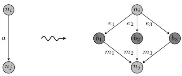
If we designate the time from the moment when a resource ceases to be needed to the end of the activity execution as “maintenance time”, then we are able to quantify the inequality of individual durations. Each resource that lies unused may carry maintenance fees: storage, lifetime decline; etc. Thus, we may conceptualize an activity as being a set of sub-activities in parallel, one per each resource, and composed of an execution phase followed by a maintenance phase. The maintenance duration for a resourcer∈Ra is simply the difference of the activity duration and the individual duration yielded by

(4)

ni ni b1 b2 b3 nj nj a e1 e2 e3 m1 m2 m3

Figure 2: WBRAS: Extended activity concept (3 sub-activities where ei are the execution phases; mi the

maintenance phases andbi the balance nodes)

By having that maintenance duration, we can apply to it a (time) unit cost; and so we can incorporate the maintenance cost into the resource allocation cost (the previously defined one). This way we ensure optimal allocations through the project total cost. It is important to notice that in order for this strategy to be correctly applied, the project must be explicitly “maintenance aware”. By this we mean that the actual project cost to be optimized must be the sum of the project cost of allocations including the maintenance costs. If we then discard the maintenance portion we would not know whether or not the allocation cost is the optimal. In fact, this strategy induces a new factor that characterizes the project. 6. Optimization Models for Multiple Resources

We base our models on the WBRAS. From this strategy we get the maintenance durations depending on

the activity duration, which is a random variable. Thus, the maintenance duration is a random variable and, consequently, the maintenance cost is also a random variable.

Since theDP-based approach is based upon decisions made accordingly to stages, we must take care of both the randomness nature and the dependency of the maintenance duration/cost. On the other hand, theGOA-based model is quite straightforward. In the next two sections we explain the two models. 6.1.DP-Based Model

This section assumes previous background knowledge of the references cited in section 4 on page 1. All the random variables present on the model are, ultimately, dependent on the work content of the resources. So, by creating representative samples for those work contents, we can derive samples for all the other random variables.

A representative sample of sizenof a work contentW ∼Exp (λ) is created by evaluating the sample valuesωi, i= 1, . . . , n where each one has probability equal to 1/n and

E[{ωi|i= 1, . . . , n}] =

ω1+· · ·+ωn

n =

1

λ =E[W] (6)

One way of describing the relationship between an activity duration and its maintenance cost is through the following set, for an arbitrarily fixed activity allocation vector:

Φa= ( ψ, X i∈Ra (si(ψ−ψi)) ! ψ= max i∈Ra  ψi  ,∀ψi∈Yai ) (7) Each Ya

i is a sample of an individual duration resulting from the allocation of each resource i to

activity a. ψ represents a sample value of the maximum of the individual durations, hence a sample value of Ya. The si values are the maintenance cost per unit time of each resource. Thus, each

element of Φaassociates an activity duration sample value (the first component of the element) with the

maintenance cost (the second component of the same element). Each one of elements in Φawill be named

asDC-Pair(Duration-Cost Pair) and the ensemble represents the sample values of the relation between the activity duration and the maintenance cost. Each pair has the probability of realization equal to the probability of the first component because of the strict relationship between the two components of each pair in Eq. (7).

The sample Φayields a distribution of the two parameters involved in theDC-Pair. This distribution

approximates the real distribution of these parameters and the approximation improves with increase in the sample size.

(5)

For the evaluation of the realization times of the nodes on the _AoArepresentation, we need to cope with the newly defined Φa,∀a∈A. More precisely, the realization of a node must contemplate the new

factor – maintenance cost. Consequently, the states now must be vectors of DC-Pair instead of only realization times. Thus, given such a state1_s

lwe want to estimate the realization of a node. To achieve

that estimation we must know the distributions for the activities which connect the state nodes to the target one. But then we need to specify that transition. Thus when, say, we go from state node n to nodek through activityawe must add the activity duration to the realization time of the node nand store the maintenance cost of the activity, hence the following equation:

Φ[n,a] ={(αn+αa, βa)|∀(αa, βa)∈Φa},(αn, βn) state on noden (8)

Notice that we do not want to add the maintenance cost of the state node. This will ensure that no cost is duplicated further on.

The actual estimation on the realization of a node will be determined from one of two scenarios. If the node is already contemplated on the state, then nothing is to be determined (its realization is already known). Else, we must set its realization time as the maximum of all the “arriving” activities contributions (durations) and add all the maintenance costs from them. Already on Eq. (8) we described the transition from a state node through an (arriving) activity to another node. Now, we must have a function that wraps those transitions in order to describe the above behavior:

DCmax  Φ1, . . . ,Φn  = ( n max i=1  αi  , n X i=1 βi ! ∀(αi, βi)∈Φi ) (9)

Hence, the estimate realization of a nodek (denoted asΥk), given a statesl is:

Υk=

 



{(αk, βk)} , nodekcontemplated on statesl

DCmax (n,a)∈P  Φ[n,a]   , otherwise (10)

where (αk, βk) is the state on node k case it is contemplated on state sl and P is the AoA network part preceding node k, with each element representing a predecessor node and the activity on the arc connecting it to nodek.

The cost of resource utilization in an activity (referred to as “the quantity cost of an activity”) is evaluated differently from the maintenance cost. So, letCa

Q be the quantity cost of activitya:

Ca Q= X r∈Ra (cr×xar×W a r) (11)

Let F denote the set of all “fixed activities” (those which resources’ allocation are not decision variables but rather fixed), the resource quantity cost of the fixed activities (denoted by rcfQ) is given

by rcfQ=E " X a∈F Ca Q # =X a∈F X r∈Ra (cr×xar× E[W a r]) (12)

Finally, indexing the decision activities by their stage, the first stage formula for theDP-based model is: f1(s1|F) = rcfQ+ min X1    E C1 Q+E sumpair cL×˙ U     (13)

whereU reflects the tardiness of the project:

U=DCmax0,Υn−T



 (14)

where Υn represents the realization of the last node andΥn−T means subtracting the constantT to

all of the first components of the elements of Υn. The notation hwhen h is a constant refers to the 1_{We use the same notation for both maintenance cost per unit time and states. That should not pose a problem as the}

(6)

DC-Pairdistribution composed by only one element (of probability 1) in which the first component is equal tohand the second equal to zero. Thus

0 ={(0,0)} T ={(T,0)} (15)

The function ˙× multiplies cL with the first component of each element of U; resulting in a new

distribution whose elements associate the tardiness cost (fist component) to the maintenance cost (second component). Then, the function sumpair adds those two costs on each element; thus resulting in a distribution whose elements are the sums. Both ˙×and sumpair do not alter the probability of the initial pairs. So, the probability of each sum is equal to the one of the original pair.

The formula for stagesk >1 is2_:

fk(sk|F) = X (α,β)∈s0 k β+ min Xk    E Ck Q+E[fk−1(sk−1|F)]     (16) wheres0

k =sk\sk−1. Then, the main formula of the model is:

f(sK = 0) = min F  fK(sK|F)   (17)

where sK = 0 means the initial state. This is associated with the initial node and represents zero

duration and zero maintenance cost. 6.2.GOA-Based Model

The GOAimplementations will rely on the Monte Carlo Simulation over the work contents. Thus, for the evaluation of the total project cost it is only required to process the realization (execution and maintenance durations) of each node; evaluate the total maintenance cost and add it to the tardiness cost and quantity allocation cost. Because of the random nature of the choice of values for the work contents, we no longer have to deal with random variables. Thus the model is linear.

Let us denote byCa

Mthe maintenance cost associated of the activitya∈A evaluated as:

Ca

M=

X

r∈Ra

(sr×(Ya−Yar)) (18)

Recall from above evaluation of Ca

Q andΥn that both involve deterministic values in this context.

TheGOAwill minimize the following function:

f =X a∈A Ca Q+C a M +cL× max  0,Υn−T   (19) 7. Implementation on Java

The models were implemented inJava1.6. A single command line application was created to deal with all the models and runtime specifications: optimization engine; with or without parallel exploitation; engine configurations; etc.

7.1.AoARepresentation

A complete library forAoAnetwork manipulation, including basic construction, was implemented to deal with the new activities with multiple resources.

7.2. Distributions

To help work with distributions, a complete library of classes was implemented. These can sample a continuous distribution or even create a partition of a given interval. For example, one of the classes can create sample distributions of the exponential distribution with arbitrary number of sample values. Also, the classes allow operations like the sum or maximum of distributions.

2_{For ease of notation we make an abuse of language: despite}_s

kbeing a vector we address each of its components as it were a set; hence the use of∈and set difference.

(7)

7.3. Combinatorics

The frequent need for walking through all the possible combinations of a number of (partitioned) variables led to the creation of classes providing linear addressing of those. Thus, instead of computing complex nesting “for” cycles, we can simply walk from the first combination to the last, deterministically and linearly. Also it is possible to process asynchronously subsets of the combinations: useful for distributed systems.

7.4.DPModel Specifics

The implementation of theDP model follows the natural recurrence of the model. This brings weaker performance to the application but achieves more accurate results.

7.5.GOAModel Specifics

BothEMAandEVAuse entities mapped as vectors. This causes a problem when applied to activities with multiple resources. Thus, instead of representing each activity on each vector component, we concatenate all the allocation vectors of the activities and mark the start and end locations. TheGOAproceeds like usual and at the end we re-assemble the activities allocation vectors.

The EMA algorithm was adapted from the original imperative-oriented form to an object-oriented form; allowing easy addition of improvements like the concurrent programming. TheEVAalgorithm was also tuned up.

7.6. Parallelism Exploitation

TheDPAcan be divided in several independent tasks: one per each allocation combination of the fixed activities. Also, theGOAinvolve several replication runs before giving the final (better) result. Thus, we enable these tasks to be processed concurrently.

For the GOA, usually the evaluation of theOF(Objective Function) value is not immediately required as other operations need to be performed first. For example, in theEMAthe computation of the forces do not take all the OF values at once; and on the EVAthe OF values are only required at the time of selection. We exploited this fact by enabling the OF value evaluation to be asynchronous. That is, instead of evaluating one-at-a-time without doing nothing else; it is possible to instruct each entity to evaluate its ownOFvalue while the main process continues the underlying operations. Later, when the

OFvalues are actually needed they will (hopefully) be ready; otherwise the main process waits (but only as needed, not always).

8. Results

The implementation was tested on Windows Vista with Java virtual machine 1.6 at 64 bits. The processor was aDuo T7300and2GBof RAM. All the tests still running after 5 hours were canceled.

All the tested projects have all the resources with the allocation interval set as [0.5,1.5]. The tests cover the application of theDPA,EMAandEVAat both single-thread and multi-thread mode. Also, two different configurations were applied on the EMAand EVA: k = 500 andk = 5000. K is the number of random values used for the work contents (Monte Carlo Simulation). TheDPAwas performed with work content sample sizes of 4 elements.

The results between single-threaded and multi-threaded runs were consistent with each other. For brevity, we only present one allocation vector (the one resulting from the single-threaded run) for both cases. The allocation vectors are presented respecting the natural order of the resources indexation. For example, if an activitya has the resourcesr1, r3and allocation vector Xa= (1,2) then xa1= 1,xa3= 2.

The DPA outputs allocation vectors for the first decision activity and for all the fixed activities. The difference between the decision and fixed allocation vectors is made through the use of Xa ={1,2} for

the decision activities and Xa = (1,2) to all the others.

(8)

8.1. Test A 1 2 3 a1 a3 a2

Figure 3: AoATopology with 3 activities and 3 nodes

Table 1: Project A.a – Single Resource

T= 16 cL= 2 a1 a2 a3 λa 1 0.2 0.1 0.07 cr sr r1 1.0 0.0

Table 2: Project A.a – Runtime Statistics

DPA EMA(k= 500) EMA(k= 5000) EVA(k= 500) EVA(k= 5000) Linear 0:00:00.203 0:00:01.450 0:00:05.445 0:00:01.294 0:00:04.977 Concurrent 0:00:00.171 0:00:00.889 0:00:03.385 0:00:01.450 0:00:03.728

Table 3: Project A.a – Allocation Results

a1 a2 a3 OFvalue DPA {1.0} (1.0) 43.7 EMA(k= 500) (0.911) (0.888) (0.851) 37.531 EMA(k= 5000) (0.872) (0.911) (0.854) 38.988 EVA(k= 500) (0.874) (0.887) (0.84) 37.291 EVA(k= 5000) (0.892) (0.879) (0.841) 38.68

Table 4: Project A.b – Multiple Resources (configuration one)

T= 41 cL= 2 a1 a2 a3 λa 1 0.07 0.09 λa 2 0.1 0.04 λa 3 0.2 cr sr r1 1.0 1.0 r2 1.1 2.0 r3 1.0 0.5

Table 5: Project A.b – Runtime Statistics

Table 6: Project A.b – Allocation Results

a1 a2 a3 OFvalue DPA {1.5,1.0,1.0} (0.5) 113.147 EMA(k= 500) (1.164,0.814,0.5) (1.096) (0.5) 84.742 EMA(k= 5000) (1.223,0.856,0.501) (1.102) (0.501) 88.108 EVA(k= 500) (1.195,0.836,0.5) (1.087) (0.5) 84.335 EVA(k= 5000) (1.118,0.782,0.5) (1.113) (0.5) 87.234

Table 7: Project A.c – Multiple Resources (configuration two)

T= 61 cL= 2 a1 a2 a3 λa 1 0.1 0.03 λa 2 0.2 0.06 0.07 λa 3 0.03 0.09 λa 4 0.04 0.04 0.07 cr sr r1 1.0 1.0 r2 1.1 2.0 r3 1.0 0.5 r4 2.0 0.1

Table 8: Project A.c – Runtime Statistics

DPA EMA(k= 500) EMA(k= 5000) EVA(k= 500) EVA(k= 5000) Linear >5h 0:00:07.660 0:00:58.812 0:00:03.978 0:00:29.160 Concurrent >5h 0:00:04.410 0:00:31.153 0:00:03.339 0:00:16.680

(9)

Table 9: Project A.c – Allocation Results a1 a2 a3 OFvalue DPA aborted EMA(k= 500) (0.568,0.5,1.421) (1.072,0.547,1.072,0.804) (0.64,0.504,0.64) 274.8 EMA(k= 5000) (0.557,0.5,1.393) (1.053,0.536,1.054,0.79) (0.621,0.507,0.622) 281.107 EVA(k= 500) (0.533,0.5,1.331) (1.048,0.542,1.048,0.786) (0.523,0.5,0.523) 269.528 EVA(k= 5000) (0.507,0.5,1.267) (1.058,0.533,1.058,0.805) (0.542,0.5,0.567) 276.860 8.2. Test B 1 2 3 4 5 a1 a2 a3 a4 a5 a6 a7

Figure 4: _AoATopology with 7 activities and 5 nodes

Table 10: Project B.a – Single Resource

T = 66 cL= 5 a1 a2 a3 a4 a5 a6 a7 λa 1 0.08 0.06 0.09 0.05 0.07 0.03 0.04 cr sr r1 1.0 0.0

Table 11: Project B.a – Runtime Statistics

Table 12: Project B.a – Allocation Results

a1 a2 a3 a4 a5 a6 a7 OFvalue DPA {1.5} (1.0) (1.0) (1.5) 205.541 EMA(k= 500) (1.364) (0.87) (1.117) (0.882) (1.127) (1.053) (1.319) 209.633 EMA(k= 5000) (1.265) (0.872) (1.209) (0.894) (1.093) (1.027) (1.301) 218.927 EVA(k= 500) (1.415) (0.939) (1.249) (0.891) (1.064) (1.024) (1.316) 209.182 EVA(k= 5000) (1.432) (0.925) (1.201) (0.886) (1.075) (1.055) (1.374) 216.076

Table 13: Project B.b – Multiple Resources (configuration one)

T= 129 cL= 5 a1 a2 a3 a4 a5 a6 a7 λa 1 0.02 0.04 0.03 0.04 0.07 λa 2 0.08 0.04 0.06 0.05 0.08 cr sr r1 1.0 1.0 r2 1.1 2.0

Table 14: Project B.b – Runtime Statistics

Table 15: Project B.b – Allocation Results

a1 a2 a3 a4 a5 a6 a7 OFvalue DPA {1.5,0.75} (1.0) (0.5) (1.0) 393.297 EMA(k= 500) (1.5,0.5) (0.5) (1.5) (0.5) (1.339,0.804) (0.658) (1.104,0.966) 361.883 EMA(k= 5000) (1.5,0.5) (0.5) (1.5) (0.5) (1.272,0.763) (0.643) (1.146,1.002) 376.068 EVA(k= 500) (1.5,0.5) (0.5) (1.499) (0.5) (1.274,0.764) (0.659) (1.22,1.068) 360.236 EVA(k= 5000) (1.5,0.5) (0.5) (1.484) (0.5) (1.282,0.769) (0.651) (1.191,1.043) 374.425

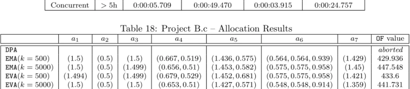
Table 16: Project B.c – Multiple Resources (configuration two)

T= 155 cL= 5 a1 a2 a3 a4 a5 a6 a7 λa 1 0.04 0.02 0.04 0.07 λa 2 0.02 0.07 0.04 λa 3 0.03 0.09 0.05 0.024 cr sr r1 1.0 1.0 r2 1.1 2.0 r3 1.0 0.5

(10)

Table 17: Project B.c – Runtime Statistics

DPA EMA(k= 500) EMA(k= 5000) EVA(k= 500) EVA(k= 5000) Linear >5h 0:00:10.904 0:01:32.493 0:00:05.522 0:00:48.126 Concurrent >5h 0:00:05.709 0:00:49.470 0:00:03.915 0:00:24.757

Table 18: Project B.c – Allocation Results

a1 a2 a3 a4 a5 a6 a7 OFvalue DPA aborted EMA(k= 500) (1.5) (0.5) (1.5) (0.667,0.519) (1.436,0.575) (0.564,0.564,0.939) (1.429) 429.936 EMA(k= 5000) (1.5) (0.5) (1.499) (0.656,0.51) (1.453,0.582) (0.575,0.575,0.958) (1.45) 447.548 EVA(k= 500) (1.494) (0.5) (1.499) (0.679,0.529) (1.452,0.681) (0.575,0.575,0.958) (1.421) 433.6 EVA(k= 5000) (1.5) (0.5) (1.5) (0.653,0.51) (1.427,0.571) (0.548,0.548,0.914) (1.359) 441.731

9. Discussion and Conclusion

For small networks with few resources, theDPAis acceptable and is even faster than theGOAwith large samples (high k). But, as soon as the networks grow by the number of resources the DPAquickly rises to run times far beyond 5 hours, while theGOAstay between few seconds to a couple of minutes; even with very largek. TheEVAis the algorithm that results in the best performance.

The performance of all algorithms reflects the benefits of the concurrent programming.

The resulting allocations and OFvalues obtained by the several algorithms are consistent with each other.

The large k= 5000 showed no improvement on the results produced with theGOA.

We conclude that the simple (recurrent) implementation of theDPAis not suitable for practical tests, while the GOA represent a good alternative in both performance and OF values (unless the detected anomalies). A new implementation of the DPAis, therefore, desirable in order to expand the spectrum of tested projects. This will enable a deep study about the presented anomalies.

10. References

[1] R. Moutinho. Gestão de Projectos – Aloca¸cão de Múltiplos Recursos. Relatório de estágio, Univer-sidade do Minho, December 2007.

[2] A. P. Tereso, M. M. T. Ara´ujo, and S. E. Elmaghraby. Adaptive Resource Allocation in Multimodal Activity Networks. International Journal of Production Economics, 92(1):1–10, November 2004. [3] A. P. Tereso, M. M. T. Ara´ujo, and S. E. Elmaghraby. The Optimal Resource Allocation in Stochastic

Activity Networks via the Electromagnetism Approach. Ninth International Workshop on Project Management and Scheduling (PMS’04), April 2004.

[4] A. P. Tereso, J. R. M. Mota, and R. J. T. Lameiro. Adaptive Resource Allocation to Stochastic Multimodal Projects: A Distributed Platform Implementation in Java. Control and Cybernetics Journal, 35(3):661–686, 2006.

[5] A. P. Tereso, R. A. Novais, and M. M. T. Ara´ujo. The Optimal Resource Allocation in Stochastic Ac-tivity Networks via the Electromagnetism Approach: A Platform Implementation in Java. Reykjav´ıc, Iceland, July 2006. 21st European Conference on Operational Research (EURO XXI). Submitted to the “Control and Cybernetics Journal” (under revision).

[6] A. P. Tereso, L. A. Costa, R. A. Novais, and M. T. Ara´ujo. The Optimal Resource Allocation in Stochastic Activity Networks via the Evolutionary Approach: A Platform Implementation in Java. Beijing, China, May 30 – June 2 2007. International Conference on Industrial Engineering and Systems Management (IESM’ 2007). Full paper published in the proceedings (ISBN 978-7-89486-439-0) and submitted to the “Computers and Industrial Engineering”.