Heterogeneous Systems
Ismael Galindo1, Francisco Almeida1, and Jos´e Manuel Bad´ıa-Contelles2 1 Department of Statistics and Computer Science
La Laguna University Spain
2
Department of Computer Science and Engineering Jaume I University Spain
Abstract. Parallel computing in heterogeneous environments is
draw-ing considerable attention due to the growdraw-ing number of these kind of systems. Adapting existing code and libraries to such systems is a fun-damental problem. The performance of this code is affected by the large interdependence between the code and these parallel architectures. We have developed a dynamic load balancing library that allows parallel code to be adapted to heterogeneous systems for a wide variety of problems. The overhead introduced by our system is minimal and the cost to the programmer negligible. The strategy was validated on several problems to confirm the soundness of our proposal.
1
Introduction
The spread of heterogeneous architectures is likely to increase in the coming years due to the growing trend toward the institutional use of multiple comput-ing resources (usually heterogeneous) as the sole computcomput-ing resource [1]. The performance of this kind of system is very conditioned by the strong dependence that exists between parallel code and architecture [2]. Specifically, the process of allocating tasks to processors often becomes a problem requiring considerable programmer effort [3].
We have devised a library that allows dynamic task balancing within a par-allel program running on a dedicated heterogeneous system, while adapting to system conditions during execution. This library facilitates the programmer the task of tailoring parallel code developed for homogeneous systems to heteroge-neous ones [4]. The library has been implemented in a way that does not require changing any line of code in existing programs, thus minimizing code intrusion. All that is required is to use three new functions:
– Library start:ULL_MPI_init_calibratelib()
– Library end:ULL_MPI_shutdown_calibratelib()
– Balancing function:ULL_MPI_calibrate(...)
This work has been supported by the EC (FEDER) and the Spanish MEC with the I+D+I contract number: TIN2005-09037-C02-01.
A. Lastovetsky et al. (Eds.): EuroPVM/MPI 2008, LNCS 5205, pp. 64–74, 2008. c
We validated our proposal on three test problems: matrix product [5], the Jacobi method for solving linear systems [5] and resource allocation optimization via dynamic programming algorithms [6]. The computational results show that the benefits yielded by using our balancing library offer substantial time reductions in every case. The efficiency level obtained, considering the minimum code intru-sion, makes this library a useful tool in the context of heterogeneous platforms. This paper is structured as follows: in Section 2 we introduce some of the issues that motivated this research and the main goals to achieve. Section 3 shows how to use our library and the advantages our approach yields. In Section 4 we describe the balancing algorithm used by the library and Section 5 shows the validation performed on the selected problems. We close with some conclusions and future research directions.
2
Background and Objectives
Programming on heterogeneous parallel systems is obviously architecture de-pendent and the performance obtained is strongly conditioned by the set of machines performing the computation. This means that, in most cases, the tech-niques used on homogeneous parallel systems must be reworked to be applied to systems which are not necessarily homogeneous [3,7].
Specifically, we set out to solve the problem of synchronizing parallel programs in heterogeneous architectures. Given a program developed for a homogeneous system, we hope to obtain a version that makes use of the system’s hetero-geneous abilities by allocating tasks according to the computational ability of each processing element. The simplest way to approach the problem consists on manually adapting the code as required by the architectural characteristics[8]. This approach usually implies at least a knowledge of said characteristics, such that the parallel program’s tasks can be allocated according to the computa-tional capacity of each processor. A more general approach can be obtained in the context of self-optimization strategies based on a run time model [4,9]. In this approach, an analytical model that parametrizes the architecture and the algorithm is instantiated for each specific case so as to optimize program execu-tion. This strategy is considerably more general than the previous one, though more difficult to apply since the modeling process is not trivial [10,11], nor is its subsequent instantiation and minimization for each case. A search of the lit-erature yields some generic tools such as mpC [12,13] and HeteroMPI [14,15] which provide the mechanisms that allow algorithms to be adapted to hetero-geneous architectures, but which also require more input from the user and are more code intrusive. Adaptive strategies have been also proposed in AMPI [16] and Dyn-MPI [17]. AMPI is built on Charm++ [18] and allows automatic load balancing based on process virtualization. Although it is an interesting generic tool, it involves a complex runtime environment.
Our objective is to develop a simple and efficient dynamic adaptation strategy of the code for heterogeneous systems that minimizes code intrusion, so that the program can be adapted without any prior knowledge of the architecture and
// p r o c s = Number o f p r o c e s s o r s ; m i i d = P r o c e s s ID ; n = Problem s i z e . . . d e s p l = (i n t ∗) m a l l o c( n p r o c s ∗ s i z e o f(i n t) ) ; c o u n t = (i n t ∗) m a l l o c( n p r o c s ∗ s i z e o f(i n t) ) ; n r o w s = n/n p r o c s; d e s p l[ 0 ] = 0 ; f o r (i = 0 ; i < n p r o c s; i++) { c o u n t[i] = n r o w s; i f (i) d e s p l[i] = d e s p l[i−1] + c o u n t[i−1 ] ; } w h i l e (i t < m a x i t) { f i n = d e s p l[m i i d] + c o u n t[m i i d] ; r e s i _ l o c a l = 0 . 0 ; f o r (i = d e s p l[m i i d] ; i< f i n; i++) { s u m = 0 . 0 ; f o r (j = 0 ; j < n; j++) s u m += a[i] [j] ∗ x[j] ; r e s i _ l o c a l += f a b s(s u m − b[i] ) ; s u m +=−a[i] [i] ∗ x[i] ; n e w _ x[i] = (b[i] − s u m) / a[i] [i] ; } M P I _ A l l g a t h e r v (&n e w _ x[d e s p l[m i i d] ] , c o u n t[m i i d] , M P I _ D O U B L E, x, c o u n t, d e s p l, M P I _ D O U B L E, n e w _ c o m) ; i t++; }
Listing 1.1.Basic algorithm of an iterative scheme
without the need to develop analytical models. We intend to apply the technique to a wide variety of problems, specifically to parallel programs which can be expressed as a series of synchronous iterations. To accomplish this, we have developed a library with which to instrument specific sections in the code. The instrumentation required is minimal, as it is the resulting overhead. Using this instrumentation, the program will dynamically adapt itself to the destination architecture. This approach is particularly effective in SPMD applications with replicated data. DynMPI is perhaps a tool closer to our library in terms of the objectives but it is focussed on non dedicated clusters. DynMPI has been implemented as a MPI extension and has a wider range of applicability. However, is more code intrusive since data structures, code sections and communication calls must be instrumented. It uses daemons to monitor the system, what means extra overhead, and the standard MPI execution script must be replaced by the extended version.
Our library’s design is directed at solving the time differences obtained when executing the parallel code without the necessity of extra monitoring daemons. It is based on an iterative scheme, such as that appearing in Listing 1.1, which shows a parallel version of the iterative Jacobi algorithm to solve linear systems. The code involves a main loop that executesmaxititerations where a calculation operation is performed for each iteration. Each processor performs calculations in accordance with the size of the task allocated, n/nprocs . Following this calculation, a collective communication operation is carried out during which all the processors synchronize by gathering collecting data before proceeding to the next iteration.
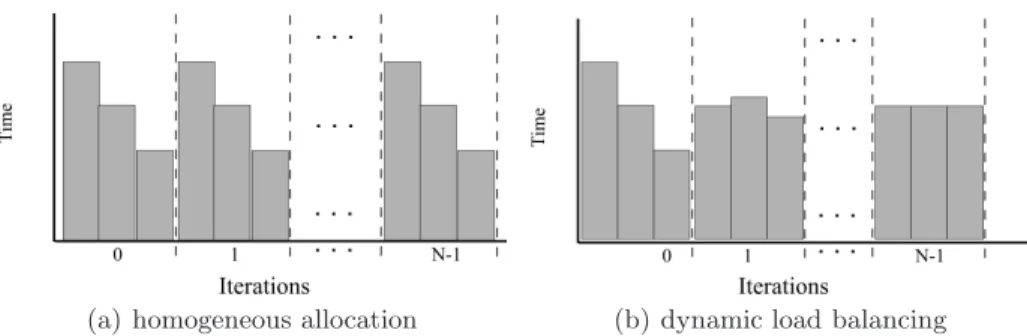
(a) homogeneous allocation (b) dynamic load balancing
Fig. 1.Time diagrams on heterogeneous systems. Each bar corresponds to the
execu-tion time of a processor on an iteraexecu-tion.
f o r (i = 0 ; i <= N; i++) { f o r (j = 0 ; j<= M; j++) { // i r r e g u l a r l o o p . I t e r a t i o n j i s O( j ) G[i] [j] = (∗f) (i, 0 ) ; f o r (x = 0 ; x<= j; x++) { f i j = G[i− 1 ] [j− x] + (∗f) (i, x) ; i f (G[i] [j] < f i j) G[i] [j] = f i j; } } }
Listing 1.2.Sequential algorithm for the resource allocation problem
Let’s suppose that a code like that showed in Listing 1.1 is executed on a heterogeneous cluster made up of, for example, 3 processors, such that processor 2 is twice as fast as processor 1, and processor 2 is four times as fast as processor 0. Then, implementing a homogeneous task allocation, where the same problem size is assigned to each node results in an execution time which is directly de-pendent on that of the slowest processor. Figure 1(a) shows the results with a problem size 1500 and with subproblems of size 500. In this case the slowest processor that determines the execution time is processor 0.
A typical solution to this problem consists of allocating on each processor a static load proportional to the its computational capacity. However, several reasons brought us to consider the dynamic strategy. The allocation of tasks according to the computational power of the processors depends on the pro-cessors and also on the application. This fact involves some benchmarking to determine the computational power of the processors and usually it is highly code intrusive. On the other hand, when facing the parallelization of codes with non-regular loops (see code of the resource allocation in Listing 1.2), the static proportional allocation is not a trivial task and if performed at runtime, the overhead introduced may not be negligible.
The next section details the strategy used for balancing task allocation with a low overhead for the execution time of each processor.
// p r o c s = Number o f p r o c e s s o r s ; m i i d = P r o c e s s ID ; n = Problem s i z e . . . d e s p l = (i n t ∗) m a l l o c( n p r o c s ∗ s i z e o f(i n t) ) ; c o u n t = (i n t ∗) m a l l o c( n p r o c s ∗ s i z e o f(i n t) ) ; n r o w s = n/n p r o c s; d e s p l[ 0 ] = 0 ; f o r (i=0; i< n p r o c s; i++) { c o u n t[i] = n r o w s; i f (i) d e s p l[i] = d e s p l[i−1] + c o u n t[i−1 ] ; } w h i l e (i t < m a x i t) { f i n = d e s p l[m i i d] + c o u n t[m i i d] ; r e s i _ l o c a l = 0 . 0 ; f o r (i = d e s p l[m i i d] ; i< f i n; i++) { U L L _ M P I _ c a l i b r a t e(U L L _ M P I _ I N I T, it, &c o u n t, &d e s p l,t h r e s h o l d, 1 ,n) s u m = 0 . 0 ; f o r (j = 0 ; j < n; j++) s u m += a[i] [j] ∗ x[j] ; r e s i _ l o c a l += f a b s(s u m − b[i] ) ; s u m +=−a[i] [i] ∗ x[i] ; n e w _ x[i] = (b[i] − s u m) / a[i] [i] ; } U L L _ M P I _ c a l i b r a t e(U L L _ M P I _ E N D, it, &c o u n t, &d e s p l, t h r e s h o l d, 1 , n) M P I _ A l l g a t h e r v (&n e w _ x[d e s p l[m i i d] ] , c o u n t[m i i d] , M P I _ D O U B L E, x, c o u n t, d e s p l, M P I _ D O U B L E, n e w _ c o m) ; i t++; }
Listing 1.3.Calibrated version of the basic algorithm of an iterative scheme
3
Dynamic Task Allocation
The library we developed allows for dynamic balancing with the introduction of just two calls to theULL_MPI_calibrate() function in the section of code that is to be balanced, as shown by the code in Listing 1.3. A call is introduced at the beginning and end of the section to be balanced, so that each processor can know on runtime how long it will take to execute the assigned task. The balanced load results from a comparison of this execution time for each processor and the subsequent task redistribution.
Listing 1.4 shows the interface of the calibrating function. The following ar-guments are input to the balancing function:
– section:The section is used to determine the entry point where the routine is used. It can take the following two values:
• ULL MPI INIT:Beginning of section to balance.
• ULL MPI END:End of section to balance.
i n t U L L _ M P I _ c a l i b r a t e (U L L _ M P I _ S e c t i o n s e c t i o n, i n t i t e r a t i o n, i n t ∗∗c o u n t s, i n t ∗∗d i s p l s,
i n t t h r e s h o l d,
i n t s i z e _ o b j e c t, i n t s i z e _ p r o b l e m) ;
– iteration:Indicates the iteration to be balanced. A 0 value indicates whether the program is on its first or subsequent iterations. The first iteration has a particular treatment.
– counts[], displs[]:Indicates the task size to be computed by each processor. counts[] is an integer array containing the amount of work that is processed by each processor.displs[] specifies the distance (relative to the work data vector) at which to place the data processed by each processor.
– threshold:Corresponds to a number of microseconds that indicate wheather to balance or not. The behaviour per iteration is as follows:
• LetTi be the time processori takes to execute the task assigned. • Tmax=M aximum(Ti)
• Tmin=M inimum(Ti)
• If (Tmax−Tmin)> thresholdthen balance. If not, the system has already
balanced the workload.
– size objects: The size of the data type manipulated during computation expressed as the number of elements to be communicated in the communi-cation routine, i.e, in the example of Listing 1.3, size objects is 1, since the elements of the matrix are double and in the communication routine they are communicated asMPI DOUBLEdata types.
– size problem: Corresponds to the total problem size to be computed in parallel, so the calculations of the new task sizes are consistent with the tasks allocated to each processorcounts[], displs[].
Running the synthetic code again on the previous three-processor cluster with a problem size equal to 1500 and a 100-microsecond threshold yields the following values for problem size (counts[]) and execution times (Ti):
– Iteration i = 0. The algorithm begins with a homogeneous task allocation:
• counts[proc0] = 500,T0 = 400us
• counts[proc1] = 500,T1 = 200us
• counts[proc2] = 500,T2 = 100us
• if ((Tmax = 400)−(Tmin = 100)) > (threshold = 100) then
bal-ance(counts[])
– Iteration i = 1. A balancing operation is performed automatically:
• counts[proc0] = 214,T0 = 171us
• counts[proc1] = 428,T1 = 171us
• counts[proc2] = 858,T2 = 171us
Figure 1(b) shows a diagram of the iterations required to correct the load im-balance. For this synthetic code the load distribution is exactly proportional to the hypothetical loads, but this is not necesarily true in practice.
Note the library’s ease of use and the minimum code intrusion. The only change necessary is to add calls to the functions at the beginning and end of the code to initialize and clear the memory (ULL_MPI_init_calibratelib(), ULL_MPI_shutdown_calibratelib()).
Table 1.Heterogenous platform used for the tests. All the processors are Intel (R) Xeon (TM).
Cluster 1 Cluster 2 Cluster 3
Processor Frequency Processor Frecuency Processor Frecuency
0 3.20 GHz 0, 1 3.20 GHz 0, 1 3.20 GHz
1 2.66 GHz 2, 3 2.66 GHz 2, 3, 4, 5 2.66 GHz
2 1.40 GHz 4, 5 1.40 GHz 6, 7 1.40 GHz
3 3.00 GHz 6, 7 3.00 GHz 8, 9, 10, 11 3.00 GHz
4
The Balancing Algorithm
The call to theULL_MPI_calibrate(...) function must be made by all the pro-cessors and implements the balancing algorithm. Although a large number of balancing algorithms can be found in the literature [19], we opted for a simple and efficient strategy that yielded satisfactory results. The methodology chosen, however, allows for the implementation of balancing algorithms which may be more efficient. All processors perform the same balancing operations as follows:
– The time required by each processor to carry out the computation in each iteration has to be given to the algorithm. A collective operation is performed to share these times among all processors.
• T[] = vector where each processor gathers all the times (Ti). • size problem= the size of the problem to be computed in parallel.
• counts[] = holds the sizes of the tasks to be computed on each processor.
– The first step is to verify that the threshold is not being exceeded if (MAX(T[]) - MIN(T[]))> T HRESHOLDthen, BALANCE
– The relative powerRP[] is calculated for each processor and corresponds to the relationship between the timeT[i] invested in performing the computa-tion for a sizecounts[i] versus the time taken for a computational unit as a function of the problem size,size problem:
RP[i] =countsT[i][i],0≤i≤N um procs−1;SRP =N um procsi=0 −1RP[i]
– Finally, the sizes of the newcountsare calculated for each processor:
counts[i] =size problem∗ RP[i] SRT
Once thecountsvector is computed, thedisplsvector is also updated. Using this method, each processor fits the size of the task allocated according to its own
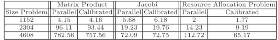
Table 2.Overhead of the calibration running on an homogeneous system with 8
pro-cessors Intel (R) Xeon (TM) 3.2 GHz
Matrix Product Jacobi Resource Allocation Problem
Size Problem Parallel Calibrated Parallel Calibrated Parallel Calibrated
1152 4.15 4.16 5.68 6.18 2 1.77
2304 96.11 93.44 19.23 19.76 14.23 9.19
computational capacity. The system could be extended to run on heterogeneous non dedicated systems and on systems with dynamic load. For that purpose, the arrayT[] must be fed not only with the execution times but with the loading factor on each processor.
To test the overhead introduced by our tool, we have executed classical parallel codes and the calibrated instrumented versions on an homogeneous system with 8 Intel 3.20 GHz processors. The parallel codes perform block assignments of the tasks with blocks of the same size for each processor. Since we are dealing with an homogeneous system, no performance improvement should be achieved and the differences in running times represent the overhead introduced. Table 2 shows the running times in each case. The overhead introduced by the tool is negligible. Note that in the resource allocation problem, the performance is improved by the code using the calibration tool. This is due to the fact that an homogeneous block data distribution is not the best choice in this case.
5
Computational Results
To check the advantages of the proposed method, we carried out a compre-hensive computational experiment where the three aforementioned applications were balanced on different heterogeneous systems. The tests were run on three clusters (Table 1) to check the library’s response to an increase in the number of processors with varying computational capacities. For the sake of the simplicity, the clock frecuency is the indicator of the level of heterogeneity, however it is a well known fact that better adjustments can be done by executing representative samples of the applications to determine the speeds of the processors. We will first analyze the performance of the resource allocation problem. Four algorithms were implemented: sequential and parallel homogeneous, heterogenous and cal-ibrated. All parallel versions of the algorithm were run on the three clusters, giving the following results:
– Tseq: Time in seconds of the sequential version.
– Tpar: Time in seconds of the parallel version, homogeneous data distribution.
– Thet: Time in seconds of the parallel version, static heterogeneous data
dis-tribution proportional to the computational load.
Table 3.Results for the Resource Allocation Problem
ClusterSize Tsec Tpar Thet Tcal GRpar GRhet
1152 7.59 7.04 4.41 3.38 51.98 23.31 1 2304 60.44 55.36 33.35 22.62 59.14 32.18 4608 483.72 430.37 257.98 168.22 60.91 34.79 1152 7.59 4.35 6.1 3.92 9.68 35.7 2 2304 60.54 30.70 20.64 23.94 22.01 -15,97 4608 483.72 237.75 139.06 121.77 48.19 12,43 1152 7.59 5.32 4,68 4.30 19.17 8,18 3 2304 60.54 24.81 20.41 18.90 23.82 7.38 4608 483.72 167.04 113.54 95.89 42.59 15.55
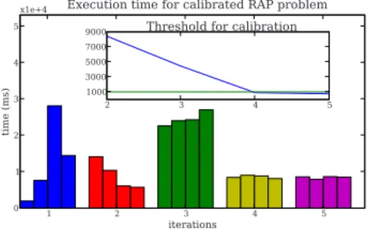
1 2 3 4 5 iterations 0 1 2 3 4 5 time (ms)
x1e+4 Execution time for calibrated RAP problem
2 3 4 5
1000 3000 5000 7000
9000 Threshold for calibration
Fig. 2.Execution time per iteration for the Resource Allocation Problem on cluster 1
(four processors) with a size of 2304
– Tcal: Time in seconds of the balanced parallel version.
– GRpar=
Tpar−Tcal
Tpar ∗100: Gain relative to the homogeneous version.
– GRhet= ThetThet−Tcal ∗100: Gain relative to the heterogeneous version.
In the calibrated version, the calibrating function was only added where appro-priate, without altering the code from the parallel version. The sequential version was executed on the fastest processor within each cluster. The threshold is prob-lem dependent and for testing purposes has been stated experimentally. The results are shown in Table 3 and are expressed in seconds. A 100-microsecond threshold was used for the calibrating algorithm. We observe important per-formance gains when using our tool. Only in one case our tool worsened the performance, and that is likely due to the threshold used in this case.
Figure 2 shows the results obtained after each iteration on cluster 1 (four processors) with a problem size of 2304. Each bar represents the execution time for each processor. Note that the times in iteration 0 of processors 2 and 3 are much higher than the rest due to the unbalanced execution. The calibration redistributes the workload, placing a higher load on processors 0 and 1 and de-creasing the load on processors 2 and 3. The problem gets calibrated at iteration 4 when using a 1000–milliseconds threshold.
Table 4.Results for the matrix product and for the Jacobi method
Matrix Multiplication Jacobi Method
ClusterSize Tsec Tpar Tcal GR Size Tsec Tpar Tcal GR
1152 30.98 47.21 18.94 59.8 1152 34.76 30.26 14.77 51.18 1 2304 720.81 400.49 248.46 37.9 2304 138.74 116.44 50.71 56.44 4608 5840.44 3344.19 2035.84 39.1 4608 553.46 463.89 190.74 58.88 1152 30.98 29.92 15.36 48.6 1152 34.76 17.54 17.05 2.79 2 2304 720.81 247.98 184.62 25.5 2304 138.74 63.43 53.44 15.74 4608 5840.44 2239.31 1639.96 26.7 4608 553.46 256.80 220.49 14.13 1152 30.98 20.009 15.42 22.9 1152 34.76 19.79 14.37 27.38 3 2304 720.81 165.40 134.15 18.8 2304 138.74 54.02 39.38 27.10 4608 5840.44 1487.51 1093.37 26.5 4608 553.46 178.81 162.53 9.10
For the matrix product and Jacobi cases the tests used square matrices of sizeSize∗Size. A threshold of 2000 microseconds was chosen for the balancing algorithm. Problem size used was a multiple of the number of processors selected. The results are shown in Table 4. Note the significant gain resulting from the dynamic balancing, which in some cases exceeds 50%. For the Jacobi method a 100-microsecond threshold was chosen for the calibrating algorithm.
6
Conclusions and Future Research
We have developed a library to perform dynamic load balancing in heterogeneous systems. The library can be applied to a wide range of problems and the effort required by the programmer is minimal, since the approach taken involves min-imum intrusion in the user’s code. In future work we plan to widen the library’s applicability to other types of programs and systems.
References
1. Top500 Org: Systems under development (2006), http://www.top500.org/orsc/2006/comes.html
2. Dongarra, J., Bosilca, G., Chen, Z., Eijkhout, V., Fagg, G.E., Fuentes, E., Lan-gou, J., Luszczek, P., Pjesivac-Grbovic, J., Seymour, K., You, H., Vadhiyar, S.S.: Self-adapting numerical software (sans) effort. IBM Journal of Research and De-velopment 50(2-3), 223–238 (2006)
3. Kalinov, A., Lastovetsky, A.L., Robert, Y.: Heterogeneous computing. Parallel Computing 31(7), 649–652 (2005)
4. Cuenca, J., Gim´enez, D., Martinez, J.P.: Heuristics for work distribution of a homo-geneous parallel dynamic programming scheme on heterohomo-geneous systems. Parallel Comput. 31(7), 711–735 (2005)
5. Wilkinson, B., Allen, M.: Parallel Programming: Techniques and Applications Us-ing Networked Workstations and Parallel Computers. Prentice Hall, Englewood Cliffs (2004)
6. Alba, E., Almeida, F., Blesa, M.J., Cotta, C., D´ıaz, M., Dorta, I., Gabarr´o, J., Le´on, C., Luque, G., Petit, J.: Efficient parallel lan/wan algorithms for optimization. The mallba project. Parallel Computing 32(5-6), 415–440 (2006)
7. Kalinov, A.: Scalability of heterogeneous parallel systems. Programming and Com-puter Software 32(1), 1–7 (2006)
8. Aliaga, J.I., Almeida, F., Bad´ıa-Contelles, J.M., Barrachina-Mir, S., Blanco, V., Castillo, M.I., Dorta, U., Mayo, R., Quintana-Ort´ı, E.S., Quintana-Ort´ı, G., Rodr´ıguez, C., de Sande, F.: Parallelization of the gnu scientific library on het-erogeneous systems. In: ISPDC/HeteroPar, pp. 338–345. IEEE Computer Society, Los Alamitos (2004)
9. Almeida, F., Gonz´alez, D., Moreno, L.M.: The master-slave paradigm on hetero-geneous systems: A dynamic programming approach for the optimal mapping. Journal of Systems Architecture 52(2), 105–116 (2006)
10. Wu, X.: Performance Evaluation, Prediction and Visualization of Parallel Systems. Kluwer Academic Publishers, Dordrecht (1999)
11. Al-Jaroodi, J., Mohamed, N., Jiang, H., Swanson, D.R.: Modeling parallel applica-tions performance on heterogeneous systems. In: IPDPS, p. 160. IEEE Computer Society, Los Alamitos (2003)
12. Lastovetsky, A.: Adaptive parallel computing on heterogeneous networks with mpc. Parallel computing 28, 1369–1407 (2002)
13. mpC: parallel programming language for heterogeneous networks of computers, http://hcl.ucd.ie/Projects/mpC
14. Lastovetsky, A., Reddy, R.: Heterompi: Towards a message-passing library for het-erogeneous networks of computers. Journal of Parallel and Distributed Comput-ing 66, 197–220 (2006)
15. HeteroMPI: Mpi extension for heterogeneous networks of computers, http://hcl.ucd.ie/Projects/HeteroMPI
16. Huang, C., Lawlor, O., Kale, L.: Adaptive mpi (2003)
17. Weatherly, D., Lowenthal, D., Lowenthal, F.: Dyn-mpi: Supporting mpi on non dedicated clusters (2003)
18. charm++ System,
http://charm.cs.uiuc.edu/research/charm/index.shtml#Papers
19. Bosque, J.L., Marcos, D.G., Pastor, L.: Dynamic load balancing in heterogeneous clusters. In: Hamza, M.H. (ed.) Parallel and Distributed Computing and Networks, pp. 37–42. IASTED/ACTA Press (2004)