http://eprints.whiterose.ac.uk/119290/
Version: Accepted Version
Article:
Worden, K orcid.org/0000-0002-1035-238X, Baldacchino, T, Rowson, J
orcid.org/0000-0002-5226-680X et al. (1 more author) (2016) Some Recent Developments
in SHM Based on Nonstationary Time Series Analysis. Proceedings of the IEEE, 104 (8).
pp. 1589-1603. ISSN 0018-9219
https://doi.org/10.1109/JPROC.2016.2573596
© 2016 IEEE. Personal use of this material is permitted. Permission from IEEE must be
obtained for all other users, including reprinting/ republishing this material for advertising or
promotional purposes, creating new collective works for resale or redistribution to servers
or lists, or reuse of any copyrighted components of this work in other works. Reproduced
in accordance with the publisher's self-archiving policy.
[email protected] https://eprints.whiterose.ac.uk/ Reuse
Unless indicated otherwise, fulltext items are protected by copyright with all rights reserved. The copyright exception in section 29 of the Copyright, Designs and Patents Act 1988 allows the making of a single copy solely for the purpose of non-commercial research or private study within the limits of fair dealing. The publisher or other rights-holder may allow further reproduction and re-use of this version - refer to the White Rose Research Online record for this item. Where records identify the publisher as the copyright holder, users can verify any specific terms of use on the publisher’s website.
Takedown
If you consider content in White Rose Research Online to be in breach of UK law, please notify us by
! " # $ % $ & ! ' ( % $ ) " * + $, - . # ( $ (( "* $ / * ( , - . # ( $ (( "* $ 0 " $ * 1 , - . # ( $ (( "* $ * 2 $, - . # ( $ (( "* $ + #/ " 3 $ * " * 4 " . . * * 5 " * 4 #* * 0 # 6 ( 6
REVIEW COPY
Response to Referees
We would like to thank the anonymous referees for their comments. We have amended the
manuscript in response and believe it has improved as a result; we hope that the revised paper
will be acceptable for publication.
Reviewer #1
This paper summarizes some examples where state-of-the-art time series analysis procedures
are applied to structural health monitoring (SHM) problems. This study is not a comprehensive
review of time series analysis as it applies to SHM as duly noted by the authors on page 3.
However, it does address what is probably the biggest challenge for all SHM methods, which
the authors refer to as “confounding influences.” Several procedures to deal with different types
of confounding influences are presented and illustrated with experimental data. Some
outstanding research issues are also presented. This reviewer believes that this paper is most
appropriate for this special issue of IEEE Proceedings. Listed below are some minor issues that
the authors should address in a revision prior to final submittal.
1.
Page 1, column 1, Line 40. I think the real assumption is that the structure is not
changing during the measurement process and, hence, the data can be associated
with a time t
Response: With respect, this is not correct. We anticipate that the structure will be changing
during the acquisition period for the training data. This is because there will be environmental or
operational variations during the training period. The main assumption is that the structure
remains undamaged during the collection of training data. We have not made changes.
2.
Page 1, column 1, Line42. AS stated it implies that different sensor reading
time-histories will be concatenated into a single vector? My assumption would that be
that each of the time histories would form a column or row of a matrix?
Response: At a given instant in time , the feature vector may indeed contain components
from more than one sensor. Over the different samples, these vectors form a set; this is as
much structure as we wish to impose at this point. In the application of certain algorithms, it may
be advantageous to assemble the vectors row-wise into a matrix. We have not made changes.
3.
Page 1, column 1, Line52, The sentence beginning “Data-based SHM is ….” First, the
authors haven’t defined what they mean by “Data-based SHM” I guess this term is
first alluded to in Line 44. Second, in the sentences starting on line 44 and 52, I
believe all SHM approaches make inferences based on subsequently measured
data – I don’t think such inferences are restricted to data-based approaches, at
least as this reviewer interpret the term “data-based.” It is hard for me to envision
any SHM or NDE approach that is not data based?
Response: Accepted. We have italicised the initial term to indicate that it is a definition and
modified the sentence to read:
Data-based SHM is then the process of making inferences about structural condition on
subsequently measured data, potentially without recourse to physical law-based models.
3 4 5 6 7 8 9 10 11 12 13 14 15 16 17 18 19 20 21 22 23 24 25 26 27 28 29 30 31 32 33 34 35 36 37 38 39 40 41 42 43 44 45 46 47 48 49 50 51 52 53 54 55 56 57 58 59 60
REVIEW COPY
4.
Page 2, column 1, line 46. This is minor, but at first read, I had trouble understanding
“…by the vertical axis and the vertical dashed line” I might suggest “…by the
vertical axis at the origin and the vertical dashed line at 250 samples”
Response: Accepted; the change has been made.
5.
Page 2, column 1, line 57. I think the results, particularly the wider limits, would be
more evident if Fig. 1 and 2 were plotted on the same vertical scale.
Response: With respect, we had already pointed out the wider limits in the text, so we believe
the figures are clear enough.
6.
Page 2, column 2, line 26. Unless the authors have an unnaturally intimate
relationship with their control charts, I don’t really understand how they can assess
if a chart is “happy”. I might suggest replacing “happily” with “effectively.”
Response: Accepted; the change has been made.
7.
Page 2, column 2, line52. It would lend credibility to this discussion regarding
variability of modal parameters if the authors could cite a study upon which these
numbers are based.
Response: this is a little difficult. This is an issue which is often discussed within the modal
analysis community and the 1% accuracy for natural frequencies (along with 10% accuracy for
modeshapes), is indeed accepted within that community. Finding the first paper where someone
said this, has eluded us; we could reference earlier papers by ourselves, where this statement
has gone unchallenged
but this would hardly add credibility. We have not made a change.
8.
Page 3, column 1, line44. Typo with right parentheses on Section II?
Response: Fixed.
9.
Page 3, column2, line40. I found this discussion a bit confusing. The discussion
refers to measurements 1356-2482, but Fig. 5 has time samples 0 – approx. 1200.
I assume sample points in Fig. 5 are the same as measurements in this
discussion. If my assumption is correct, I think it will help the reader if this
terminology can be made consistent and that the discussion can directly relate the
measurement numbers to the sample numbers in Fig. 5.
Response: Accepted, we have added a footnote in explanation.
In the figures, the term 'Sample Point' or 'Sample Point Number' is a general term which simply
means the points are counted from the beginning of the record plotted. In the case of Figures 8,
9, 10, 11 and 12, the sample numbers also coincide with the measurement numbers given in
the text which specify the three test phases.
10. Page 4, column2 line 22. The term “supervised learning” does not appear in the
introduction? Also, I believe the authors are using the term supervised learning in
reference to the ability to model the influence of temperature on the features.
However, it seems to me the ability to identify damage is still being done in an
3 4 5 6 7 8 9 10 11 12 13 14 15 16 17 18 19 20 21 22 23 24 25 26 27 28 29 30 31 32 33 34 35 36 37 38 39 40 41 42 43 44 45 46 47 48 49 50 51 52 53 54 55 56 57 58 59 60
REVIEW COPY
unsupervised learning mode. If I’m correct about this, I think this should be stated
explicitly.
Response: This was a typo’, we have corrected the term to ‘unsupervised learning’.
11. Page 4, column 2 line 24. In the entire discussion of the naïve analysis the authors
introduce the Mahalanobis squared distance as a measure of discordancy.
However, when I examine Figures 9, 10 and 11 it appears it is actually being used
as the damaged-sensitive feature? I think a little bit more explanation on what
distinguishes a measure of discordancy from a feature is needed in the context of
this example.
Response: The MSD is being used as a damage- or novelty index. As such it is certainly a
damage sensitive feature, but a rather trivial one. It is essentially the output of a two-class
classifier based on the actual input features. As such we prefer not to denote it has a feature.
12. Page 5, column 1 line17. I think the authors should explicitly state what level of
threshold is shown by the horizontal dashed line, 3 standard deviations from the
mean?
Response: This is given in the text, at the bottom of Page 4, Column Two, in the original
manuscript:
In this work, the threshold value is computed using the Monte Carlo method described in [11]
and corresponds to a 99\% confidence threshold unless otherwise indicated.
13. Page 6, column 2, line 2. I think more explanation is needed. If the undamaged data
has been acquired during three identical temperature cycles, why is the upward
trend only noticed at the end of the third cycle?
Response: This is a good point, and we don’t have an immediate answer. It may be that the
temperature cycles were not exactly replicated. Such drift does sometimes occur when one
moves around in the training data, even when the system is still in normal condition. The drift is
less visible in the cointegration results in Figure 12. As we have nothing more definite to say, we
have made no changes.
14. Page 6, column 2, line 23. I’m having trouble with the notation. Again, it seems like
the multivariate time series would be represented by a matrix? I’m assuming
multivariate here means the data are from multiple sensors? This seems
inconsistent with the notation used on page 1, column 1, line 50?
Response: the notation is consistent with the opening paragraph; for the sake of clarity, we have
added after equation (2),
‘and where
= ( ).
15.
Page 7, column 2, line 17. I assume the statement “..eigenvectors are assembled
columnwise into a vector, ..” should read “..eigenvectors are assembled columnwise into a
matrix,..” I suspect that this might be related to comments 2 and 14. However, if this reviewer
is having trouble with this issue, then I suspect other will as well.
3 4 5 6 7 8 9 10 11 12 13 14 15 16 17 18 19 20 21 22 23 24 25 26 27 28 29 30 31 32 33 34 35 36 37 38 39 40 41 42 43 44 45 46 47 48 49 50 51 52 53 54 55 56 57 58 59 60
REVIEW COPY
Response: This was a typo’ and is now fixed.
15. Will Figures 17, 18 and 19 be effective if printed in B&W?
Response: We believe so, we have used a dark shade, a light shade and a dashed line to help
with this. We also anticipate that the majority of readers will print the paper in colour from the
journal website.
Reviewer 2
The reviewer would first like to thank the authors for a strong contribution to the journal. The
paper is very well done and provides a very insightful contribution on co-integration methods for
non stationary systems. Major and minor comments provided below:
Response: Thank you
Major issues:
1. The title and the abstract are not related to the paper - the paper is really focused on the
use of cointegration and mixture of experts methods for time series-based analysis for
SHM. Neither term are even used in the abstract. The reviewer feels the title and
abstract should better reflect the paper content.
Response we have amended the title to:
Some Recent Developments in SHM based on Nonstationary Time Series Analysis
and we have amended the abstract as follows:
Many of the algorithms used for Structural Health Monitoring (SHM) are based on or motivated
by time series analysis. Quite often, detection methods are variants of approaches developed
within the Statistical Process Control (SPC) community. Many of the algorithms used represent
mature theory and have a rigorous probabilistic or mathematical basis. However, one of the
main issues facing SHM practitioners is that the structures of interest rarely respect the
assumptions inherent in deriving algorithms. In the case of time series data, SPC-based
approaches usually require the data to be stationary and, unfortunately, SHM data is often
nonstationary because of benign variations in the environment of the structure of interest, or
because of deliberate operational changes in the use of the structure. This nonstationarity can
manifest itself as slowly-varying trends on the data or in abrupt switches between regimes.
Recent work in nonstationary time series methods for SHM has made considerable progress in
accommodating nonstationarity and some of that work is discussed within this paper: in terms
of understanding slowly-varying trends, the cointegration algorithm from econometrics is
presented; for understanding abrupt switches, Bayesian mixtures of experts are presented.
Another issue in time series analysis is indirectly related to the assumption of linear behaviour of
structures and the impact of this assumption is briefly considered in terms of its effects on
detection thresholds in SPC-like methods; again, progress has been made recently. Some
issues still remain, and these are discussed also.
Some very minor comments for the authors:
1. Figure 7 caption references "Figure 7" when it intends to cite "Figure 6".
3 4 5 6 7 8 9 10 11 12 13 14 15 16 17 18 19 20 21 22 23 24 25 26 27 28 29 30 31 32 33 34 35 36 37 38 39 40 41 42 43 44 45 46 47 48 49 50 51 52 53 54 55 56 57 58 59 60
REVIEW COPY
Response: Corrected.
2. Figure 8 could be improved with the 3 forms of data delineated in the figure.
Response: We respectfully disagree. We feel the transitions are clear in the figure, and we have
given the points at which transitions occur in the text. If we overlay vertical lines, for example,
we will obscure features of the data.
3. Figure 5 seems to be cropped on the right.
Response: The figure is OK as a .eps file, we are unsure what happened. If the problem
persists at the proof stage, we will attempt to generate a plot without the problem.
4. Page 6, Line 8 - authors intend to say, "...for more of a SHM context." - add "of a".
Response: Corrected.
5. Page 6, Lines 31-32, Column 1 - some more discussion about data standardization is
needed here.
Response: We have added a footnote:
The process of standardisation of a given variable is simply to remove its mean and to divide by
its standard deviation. There is some disagreement on whether data should be standardised
before PCA is applied. Some argue that standardisation stops variables from dominating the
decomposition simply because they have a greater magnitude; the counter argument is that
such variables are therefore more important and should be allowed to dominate.
6. Page 6, Lines25-26, Column 2 - the authors state that if y is n-dimensional, there are up
to n-1 linearly independent cointegration vectors. Why? Can the authors elaborate?
Response: Yes
The cointegration algorithm used in the paper is, like PCA, based on an
eigenvalue problem. The first eigenvector produces the cointegrating vector which gives the
most stationary residual. The second eigenvector gives the cointegrating vector, (weighted)
orthogonal to the first, that gives the next most stationary residual, and so on. This ultimately
results in n – 1 vectors. With respect, we think that adding this argument to the paper is a
digression and we would prefer to point the reader to a reference.
7. Page 7, Line 27, Column 1 - a paranthese is accidentally added after the citation [23].
Response: Corrected.
8. Page 8, Lines 27-34, Column 1 - the description here is rather unsatisfying. Can the
authors. How does the experiment interruption map into the spike? The causality here
is not self-evident to the reviewer. Perhaps what is contained in [9] could be briefly
summarized as it pertains to the spike in Figure 12.
Response: The discussion in [9] is quite long, so we would respectfully prefer to direct the
reader towards it rather than reproduce or precis it in the current paper.
9. Citation 19 - looks like there is a typo here.
3 4 5 6 7 8 9 10 11 12 13 14 15 16 17 18 19 20 21 22 23 24 25 26 27 28 29 30 31 32 33 34 35 36 37 38 39 40 41 42 43 44 45 46 47 48 49 50 51 52 53 54 55 56 57 58 59 60
REVIEW COPY
Response: Corrected.
3 4 5 6 7 8 9 10 11 12 13 14 15 16 17 18 19 20 21 22 23 24 25 26 27 28 29 30 31 32 33 34 35 36 37 38 39 40 41 42 43 44 45 46 47 48 49 50 51 52 53 54 55 56 57 58 59 60REVIEW COPY
Some Recent Developments in SHM based on
Nonstationary Time Series Analysis
Keith Worden, Tara Baldacchino, Jennifer Rowson and Elizabeth J. Cross
(Invited Paper)
Abstract—Many of the algorithms used for Structural Health Monitoring (SHM) are based on or motivated by time series analysis. Quite often, detection methods are variants of ap-proaches developed within the Statistical Process Control (SPC) community. Many of the algorithms used represent mature theory and have a rigorous probabilistic or mathematical basis. However, one of the main issues facing SHM practitioners is that the structures of interest rarely respect the assumptions inherent in deriving algorithms. In the case of time series data, SPC-based approaches usually require the data to be stationary and, unfortunately, SHM data is often nonstationary because of benign variations in the environment of the structure of interest, or because of deliberate operational changes in the use of the structure. This nonstationarity can manifest itself as slowly-varying trends on the data or in abrupt switches between regimes. Recent work in nonstationary time series methods for SHM has made considerable progress in accommodating nonstationarity and some of that work is discussed within this paper: in terms of understanding slowly-varying trends, the cointegration algorithm from econometrics is presented; for understanding abrupt switches, Bayesian mixtures of experts are presented. Another issue in time series analysis is indirectly related to the assumption of linear behaviour of structures and the impact of this assumption is briefly considered in terms of its effects on detection thresholds in SPC-like methods; again, progress has been made recently. Some issues still remain, and these are discussed also.
I. INTRODUCTION
I
N a sense, all Structural Health Monitoring (SHM) is a matter of time series analysis; the temporal element of the activity is implicit in the term ‘monitoring’. An individual act of monitoring occurs when one or more sensors on a structure of interest are interrogated; readings are taken and recorded. For the sake of mathematical convenience, it will be assumed that the measurement is instantaneous and can be associated with a time t. It will further be assumed that more than one sensor can be interrogated at a time, so the measurement will be vector valued and will be denoted here by x(t). In a data-based, or machine learning approach to SHM [1], it is usual to monitor a structure over a period of time when it is known to be undamaged or in its normal condition; the resulting set of measurements is usually referred to as the training set. If N points of training data are observed, the training set will take the form {xi =x(ti); i= 1, . . . , N}. (Throughout thispaper, vectors will be denoted by underlines and matrices by upper case letters.) Data-based SHM is then the process of making inferences about structural condition on subsequently
All authors are with the Department of Mechanical Engineering, University of Sheffield, Mappin Street, Sheffield S1 3JD, UK.
Manuscript received April 31, 2015; revised Month 00, 2015.
measured data, potentially without recourse to physical law-based models. As the measurements will almost alway form a multivariate sequence ordered with respect to time, it follows that data-based SHM is a matter of time series analysis in its most general sense. In general, the time series will not necessarily be raw sensor measurements like accelerations, but will be pre-processedfeaturesconstructed in order to enhance damage sensitivity.
The most basic form of inference in data-based SHM is damage detection i.e. one seeks to establish only if the structure is no longer in its normal condition. This form of diagnosis is usually carried out in terms of novelty detection
or outlier analysis[1]. The idea behind these methods is that the training data are used to construct a statistical model of the structure in its normal condition. Subsequent data are tested for consistency with the statistical model and if deviations are found, the implication is that the structure has left its normal (undamaged) condition. There are many methods of novelty detection of varying levels of sophistication; however, they all suffer from a potentially serious problem - the problem of confounding influences. The problem is simply that a structure may change its condition for benign reasons e.g. it may be subject to environmental or operational variations. A simple example will suffice; suppose that the measurements, or more properlyfeatures of interest are the first few natural frequencies of the monitored structure. It is usually the case that damage will reduce the local stiffness of the structure and can also increase damping (e.g. a crack can dissipate energy through interfacial friction); both of these effects of damage will cause the natural frequencies to decrease, so natural frequencies aredamage-sensitive features. The problem is that natural frequencies are also (and more) sensitive to other benign influences like ambient temperature, wind and traffic loading (on bridges for example). The issue is then that a change in the natural frequencies from a benign cause could be attributed to damage and thus produce a costly false alarm. An effective SHM methodology may thus need a means of removing confounding influences before the diagnostic analysis is made. A good, and fairly recent, review of the issues surrounding confounding influences can be found in [2].
Fortunately, the variations due to confounding influences often have different characteristics to the signal components of interest i.e. those that expose the dynamic properties of the structure of interest, and this means they can sometime be removed. Suppose that the feature of interest is an acceleration and further suppose that the statistics of the vibration signal do not change with time i.e. the signal isstationary. While the
3 4 5 6 7 8 9 10 11 12 13 14 15 16 17 18 19 20 21 22 23 24 25 26 27 28 29 30 31 32 33 34 35 36 37 38 39 40 41 42 43 44 45 46 47 48 49 50 51 52 53 54 55 56 57 58 59 60
REVIEW COPY
which are fractions of seconds, variations due to temperature say, will occur on timescales of the order of hours; the high-frequency signal of interest will then be carried on a low-frequency trendand the combined signal is nonstationary. If the temperature is known (measured), a low-order polynomial fit to the whole data record will capture the trend and not the local dynamics and the fitted trend can then be removed. This is an example of asubtractionscheme for trend removal. If the temperature has not been measured, one must resort to other methods likeprojectionmethods. Projection methods rely on the availability of multiple features and exploit the fact that confounding influences will occupy a low-dimensional subspace of the feature space and can be projected out. The next section of this paper will discuss a recently developed projection method which seems particularly attuned to the SHM problem - the application of cointegration. In contrast to environmental variations, which often manifest as trends, operational variations tend to manifest as short timescale transients e.g. an aircraft dropping a store. Such variations may be well handled by regarding the structure as switching between different normal conditions. The problem here is that the normal condition set in feature space may have a complicated structure which then requires more sophisticated methods of novelty detection [3]–[6]. Some simple examples will serve to illustrate some of the issues discussed above. In all cases, the signals are intended to represent normal condition data.
In order to focus the discussion on the issues of non-stationarity, rather than on SHM algorithms, the detection algorithm will be assumed to be the simplest one possible. The univariate X-chart will be used from the discipline of
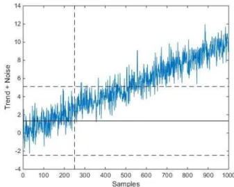
Statistical Process Control (SPC) [7]. The idea is that one observes a single sensor variable (or feature) over a training period; the mean and standard deviation of the training signal are estimated and then upper and lower control limits for the signal are derived. If subsequent measurements leave the control interval, damage is deemed to have occurred. If one assumes the the sensor signal is a Gaussian noise process, then the control limits are straightforwardly determined e.g. the mean plus or minus three standard deviations gives a 99.7% confidence interval; this means that only three from a thousand observations would leave the interval as a result of random fluctuations. To illustrate how this might work, Figure 1 shows 1000 samples from a Gaussian process with zero mean and unit standard deviation; the control limits have been estimated from the statistics of the first 250 points - the training set in this case. (In the following group of figures, the training set is delimited by the vertical axis at the origin and the vertical dashed line at 250 samples.)
This situation raises no issues; the stationarity of the signal means that the control limits are appropriate outside the training set and there are no false-positive indications of damage beyond the number expected for a 99.7% confidence interval. Now, suppose that the noise process is supplemented by a continuous linear trend as in Figure 2. This is by no means unrealistic, if the feature of interest here were a natural frequency of a bridge say, a noise component would arise as a
Fig. 1. SPC control limits for a stationary Gaussian noise process.
result of estimation errors and a trend could arise as a result of variations in the ambient temperature. If the first 250 samples are used as a training set as before, they produce wider limits as a result of the fact that the training data are nonstationary; however, because the trend continues and the training set has not captured all possible benign variations, the signal leaves the control limits soon after the training period and begins to give continuous false-positive indications of damage. If the trend could be removed, a stationary stochastic process would result and the simple SPC approach would function quite effectively.
Fig. 2. SPC X-chart for a nonstationary (linear trend) process.
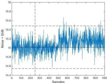
The next example illustrates switching behaviour consistent with an operational variation. This time, the example is motivated directly by reality. Suppose the measured feature is a natural frequency of an aircraft structure (which will have been extracted by processing raw accelerometer data). If the nominal value of the frequency is 15 Hz, accumulated experience with most modal analysis methods means that one would expect measurement errors of the order of 1% i.e. with
3 4 5 6 7 8 9 10 11 12 13 14 15 16 17 18 19 20 21 22 23 24 25 26 27 28 29 30 31 32 33 34 35 36 37 38 39 40 41 42 43 44 45 46 47 48 49 50 51 52 53 54 55 56 57 58 59 60
REVIEW COPY
dropping of a store from the aircraft raises the frequency by 1%. Figure 3 shows a representation of this situation over 1000 samples where the operational change occurs at point 501. As before, the control limits are estimated from training data over the first 250 samples. As in the trend case, the oper-ational variation causes many more false positive indications of damage than the 0.3% expected from the structure in the initial condition. If a model of the switching behaviour were established and the predictions subtracted from the frequency measurements, the residual error would be a stationary random process and thus appropriate for the simple SPC approach.
Fig. 3. SPC X-chart for a nonstationary (abrupt shift) process.
The remainder of this paper will illustrate how recent developments in time series analysis for SHM allow one to overcome some of the issues discussed above. The paper is not intended as a survey paper in any real sense and is very biased towards the work of the authors, simply because this is the work with which they are most familiar. The idea is to discuss some of the issues regarding time series analysis and highlight
some means of resolving them. The layout of the paper is as follows: Section II discusses how (fairly) recently developed projection methods have allowed progress on the removal of slowly varying trends from SHM data and also discusses some remaining issues. Section III considers how abrupt (but benign) changes in structural behaviour can be accommodated within SHM time series analysis. The paper then closes with some brief conclusions. The most effective algorithms shown in Sections II and III are probabilistic, but differ somewhat in their philosophy; the approach to trend removal -cointegration
- is based here on a maximum likleihood approach, while the means of dealing with switching behaviour is a Bayesian algorithm. This has been done deliberately; however, there is an impact on the reader, a complete understanding of the approach to switching behaviour here requires some familiarity with concepts from Bayesian machine learning theory. A good reference on the background to, and terminology of, Bayesian methods in machine learning can be found in [8].
PROJECTIONMETHODS A. Case Study: Experiment and Feature Selection
To illustrate the removal of counfunding influences, a case study is presented here. The context is experimental wave-based SHM; the inspection of a composite sample using Lamb waves. The material of this section has been presented elsewhere, notably in [9], where the experiment and results are discussed in much more detail. The ‘structure’ under consideration is a 300-mm-square composite laminate plate, instrumented via two piezoelectric sensors/actuators as shown in Figure 4. 300 mm 300 m m Transmitter Receiver Damage
Fig. 4. Schematic of composite plate used in case study showing the positions of the sensor/actuators and imposed damage.
The piezoelectric elements can operate in a symmetric fashion and in both pitch-catch and pulse-echo modes with the former mode adopted here. The purpose of the experiment was to examine the effects of environmental variations on SHM features. Lamb wave signals travelling between the sensor-actuator pair were recorded every minute with the plate located in an environmental chamber. In the first phase of the test, the environmental chamber was held at a temperature of 25◦C for the first 1355 measurements. In the second phase, the temperature was cycled three times between 10◦C and
30◦C (measurements 1356-2482) and the temperature in the
chamber was recorded. In the third and final phase, a hole was drilled in the plate and the temperature was again cycled between 10◦C and 30◦C (measurements 2483-2944). The
temperature profile imposed during phase 2 is shown in Figure 51.
The Lamb wave signal launched from the actuator was a five-cycle toneburst modulated by a Hanning window; the actuation frequency was chosen at 80 kHz in order to pref-erentially excite the symmetric Lamb wave mode. A typical 1In the figures, the term ’Sample Point’ or ’Sample Point Number’ is a
general term which simply means the points are counted from the beginning of the record plotted. In the case of Figures 8 9, 10, 11 and 12, the sample numbers also coincide with the measurement numbers given in the text which specify the three test phases.
3 4 5 6 7 8 9 10 11 12 13 14 15 16 17 18 19 20 21 22 23 24 25 26 27 28 29 30 31 32 33 34 35 36 37 38 39 40 41 42 43 44 45 46 47 48 49 50 51 52 53 54 55 56 57 58 59 60
REVIEW COPY
Fig. 5. Temperature profile imposed on the composite plate during the secondphase of the experiment.
example of the received signal is given in Figure 6. The features for damage detection were then obtained by Fourier transforming the time-history of the received Lamb wave signal; a typical example of a spectrum (magnitude) is given in Figure 7. In order to reduce the dimension of the feature vector, 50 spectral lines (magnitude only) around the peak in the spectrum were selected.
0 500 1000 1500 2000 2500 −0.06 −0.04 −0.02 0 0.02 0.04 0.06
Sample Point Number
Amplitude
Fig. 6. Typical waveform of the received Lamb wave signals used for SHM.
0 10 20 30 40 50 60 70 80 90 100 0 1 2 3 4 5 6 7 8 9
Spectral Line Number
Amplitude
Fig. 7. Spectra of the received Lamb wave signal corresponding to the waveform in Figure 6.
Note that there are two time-series in the feature selction process with quite different natures. The raw Lamb wave response data consists of a univariate series sampled in the MHz range; the feature selection process converts this into a multivariate (50-dimensional) series sampled once per minute.
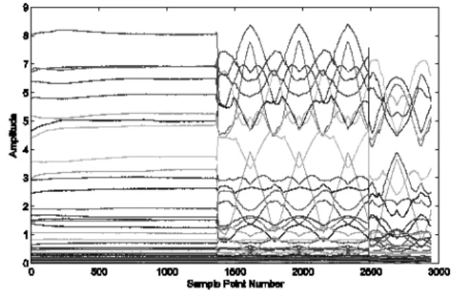
Figure 8 shows how all the spectral line features vary across the three phases of the experiment. It is clear from this figure that the variations in the features as a result of changes in the environment are of the same order of magnitude as the variations induced by damage; this represents a problem in the context of novelty detection.
Fig. 8. Features (spectral line magnitudes) for SHM shown over the three phases of the experiment.
The next subsections will illustrate how confounding in-fluences can be misleading if a naive approach to novelty detection is taken and how a more sophisticated approach can overcome the problem. It is assumed from this point on that data available for training will include some from the temperature-varying phase of the test, but none from the phase were damage was induced. This is consistent with the usual situation for unsupervised learning as discussed in the introduction.
B. Naive Analysis
The analysis in this section can be considered naive in two senses. In the first sense, the novelty detection algorithm is one of the simplest and most restricted possible. The second sense arises because it is assumed that there is no means of transforming the data into a more effective form for analysis. It will be shown later, that when the data are transformed, the simplicity of the algorithm is no longer an issue. The detection algorithm adopted here is from the discipline of
outlier analysis[10], and assesses the discordancy of a single observation with respect to the rest of the data, or a fixed set of training data. A discordant outlier in a data set is an observation that appears inconsistent with the rest of the data and therefore is believed to be generated by an alternate mechanism to the other data. A measure of discordancy is defined which allows comparison against an objective criterion allowing the outlier to be judged to be statistically likely or unlikely to have come from the assumed generating model. The discordancy test for multivariate data used here is the Mahalanobis squared-distance (MSD) measure given by [10], [11], Dζ = (xζ−x)TS− 1 (xζ−x) (1) 3 4 5 6 7 8 9 10 11 12 13 14 15 16 17 18 19 20 21 22 23 24 25 26 27 28 29 30 31 32 33 34 35 36 37 38 39 40 41 42 43 44 45 46 47 48 49 50 51 52 53 54 55 56 57 58 59 60
REVIEW COPY
ζ
the sample observations and S the sample covariance matrix. In order to label an observation as an outlier or an inlier there needs to be some threshold value against which the discor-dancy value can be compared. This value is dependent on both the number of observations and the number of dimensions of the problem being studied. The value also depends upon whether an inclusive or exclusive threshold is required. In this work, the threshold value is computed using the Monte Carlo method described in [11] and corresponds to a 99% confidence threshold unless otherwise indicated. The MSD is arguably the simplest discordancy measure as it assumes a Gaussian distribution for the normal condition data; the MSD of a test point is then essentially the log likelihood of the point belonging to the normal condition set.
The first piece of analysis here is based on a training dataset chosen as every second data point recorded when the temperature of the plate was held constant (i.e. during phase one of the experiment); this assumes that the plate under constant temperature is the normal condition. For the outlier analysis, the mean, x, and covariance matrix, S, were calculated for the 678 training set samples. All the feature samples were then in turn designatedxζand values forDζ, the
novelty index (discordancy), were calculated using equation (1). Figure 9 shows the results of this analysis, with the novelty index plotted on a log scale (note that the novelty indices of the samples in the training set are also plotted). The horizontal dotted line represents the threshold value, whereas the vertical lines separate the three regimes corresponding to the phases of the experiment. Not surprisingly, almost all of the novelty indices from samples in the constant temperature regime are below the threshold. Meanwhile, the features from the temperature cycling period and the damage set are all sub-stantially over the threshold, indicating an abnormal response from the plate for the majority of the testing period. This is clearly an undesirable situation; if the outlier analysis was to be intended as a damage detector, responses from the plate under a changing temperature would be wrongly classified as such. 0 500 1000 1500 2000 2500 3000 1 2 3 4 5 6 7 Feature Number
Log Novelty Index
Fig. 9. Outlier analysis: naive results assuming constant temperature training data.
Figure 9 provides an insight into how badly a novelty detector would work if the constant temperature data were considered to define the normal condition; the temperature fluctuations lead to a 100% rate of false-positive detection
improvement should come from including data from the un-damaged plate when the temperature was fluctuating in the training set. Figure 10 shows the results of the same outlier analysis as before, but this time with the training data extended to include data from the fluctuating temperature regime. The training dataset next used included every second data point up to data point 2000; this includes data from just under two full cycles of temperature fluctuation. The improvement in the approach is clear in Figure 10; redefining the normal condition to include data points from the temperature fluctuating regime of the experiment has clearly decreased the discordancy of the data points from this regime. However, some structure still remains visible in the MSD from the fluctuating temperature period and many points cross the threshold (indicated by the dashed line) yielding many false-positive indications of damage. The MSD is evidently nonstationary over the phase two data and thus violates the primary condition for applying any concepts from SPC; furthermore, if the data are not i.i.d and Gaussian, the threshold calculated via the procedure of [11] is inappropriate. In terms of damage detection, this outlier analysis would still be very inappropriate.
0 500 1000 1500 2000 2500 3000 1 1.5 2 2.5 3 3.5 4 4.5 5 5.5 Feature Number
Log Novelty Index
Fig. 10. Outlier analysis: naive results assuming some varying temperature training data.
C. Principal Component Analysis
Fortunately, recent years have provided new means of avoid-ing the naive analysis of the last section when confoundavoid-ing influences are present. The new methods allow the removal of the confounding influences prior to novelty detection. Broadly speaking, the removal methods fall into two categories
subtractionschemes and projectionschemes. The subtraction schemes are arguably less general in their applicability as they rely on the availability of measurements of the variables that are driving the environmental or operational variations (in this case, temperature). Subtraction methods work by fitting a re-gression model which accounts for the component of measured features dependent on the driving variable; this component can then be subtracted from the training, and any subsequent testing, data. Because they are arguably more general, the current paper will concentrate on projection methods; the reader curious about subtraction methods can consult [1], [2], or [12] which also demonstrates subtraction schemes based on interpolation rather than regression.
3 4 5 6 7 8 9 10 11 12 13 14 15 16 17 18 19 20 21 22 23 24 25 26 27 28 29 30 31 32 33 34 35 36 37 38 39 40 41 42 43 44 45 46 47 48 49 50 51 52 53 54 55 56 57 58 59 60
REVIEW COPY
gebra, applied to the multivariate feature space. They are all based on the same principle, which is that the confounding influences will occupy a subspace (hopefully low-dimensional) of the feature space; this will be referred to as the trapping subspace here. If this subspace can be computed, evidently projecting the feature data onto the subspace orthogonal to the trapping subspace will remove all of the confounding influ-ences. Two examples of projection methods will be presented here; although the methods differ in their criteria for defining the trapping subspace, the means of computation are exactly the same, both methods define an eigenvalue problem in which a subset of eignevectors span (and thus define) the trapping subspace.
The first method discussed here will be Principal Compo-nent Analysis (PCA). PCA is a very well-established method from multivariate statistics, so the background theory will not be repeated here; the reader can consult a standard textbook like [13] for the theory, or consult [1] for more of an SHM context. PCA works by linearly transforming a multivariate feature set into a set of uncorrelated variables ordered in terms of their variance (power). This means the first principal component (PC) gives the linear combination of the original features with highest variance, the second PC is the linear combinationorthogonal to the firstthat gives the next highest variance, and so on. The application to SHM is then based on the observation that the trends in the data make the higher contributions to the variance; as an illustration, if one considers the signal in Figure 2, the noise component of the signal has variance 1.0, while the trend component has variance 9.1. This motivates the definition of the trapping subspace as that spanned by the first few principal components; removal of the confounding influences is then accomplished by projection onto the remaining minor components. Historically, PCA (and the closely related Factor Analysis) were the first projection methods conceived for SHM [14], [15].
Having defined the procedure it is a simple matter to illus-trate it. The PCA algorithm was applied to the training data described above which contained examples of the temperature variations. To be more certain of capturing the confounding influences, the data were projected onto the ten smallest minor components. The results of applying outlier analysis to the projected data are shown in Figure 11. It is important to note that the data were not standardised before PCA as is commonly done2. In fact, pre-standardisation produced much
inferior results; this matter is discussed in much more detail in [9].
The results of PCA projection show a marked improvement over those shown in Figure 10; almost all of the structure is removed from the MSD over the phase two data and the number of false positives is reduced considerably. There is only really one remaining concern with the results, which is 2The process of standardisation of a given variable is simply to remove its
mean and to divide by its standard deviation. There is some disagreement on whether data should be standardised before PCA is applied. Some argue that standardisation stops variables from dominating the decomposition simply because they have a greater magnitude; the counter argument is that such variablesaretherefore more important and should be allowed to dominate.
0 500 1000 1500 2000 2500 3000 0 0.5 1 1.5 2 2.5 3 3.5 4 4.5
Sample Point Number
Log Novelty Index
Fig. 11. Outlier analysis based on PCA projection of training and testing data.
that some residual nonstationarity remains, the MSD values trend upwards towards the end of the undamaged period and finally cross the threshold, yielding a small number of false positives. As discussed above, there are other projection methods based on different definitions of the trapping subspace which might prove beneficial. In fact, one might argue that PCA is not particularly well-matched to SHM by its projection criterion; one might question why the signatures of damage are likely to reside in the minor components. In the next section a different projection method is presented which is arguably matched to SHM requirements - the application of
cointegration.
D. Cointegration
Cointegration is a property of multiple nonstationary time series [16]–[18]. In essence, two or more nonstationary time series will be said to be cointegrated if some linear com-bination of them is stationary. Symbolically, a multivariate nonstationary time seriesy
i is cointegrated if a vectorβ exists
such thatzi is stationary, where,
zi=βTyi (2)
and where y
i =y(ti).
In this situation, βT is termed a cointegrating vector. In general, there will not be a unique cointegrating vector; in fact, if y
i is n-dimensional, there may be up to n − 1
linearly independent cointegrating vectors. A more general and precise definition of cointegration requires one to introduce the concept of anorder of integration; this is the number of times one must difference a nonstationary time series before it becomes stationary. For engineering applications, most vari-ables of interest can be considered to be integrated of order 1 (denoted I(1)), which implies that their first differences will be stationary [19]. In general, a set of time series are cointegrated if they share a common order of integration and a linear combination of the variables exists with a lower order of integration. As the order of integration must be the same for cointegrated variables, the first step in a cointegration analysis will often be to ascertain the order of integration of each of the variables to be included in the analysis. This assessment is
3 4 5 6 7 8 9 10 11 12 13 14 15 16 17 18 19 20 21 22 23 24 25 26 27 28 29 30 31 32 33 34 35 36 37 38 39 40 41 42 43 44 45 46 47 48 49 50 51 52 53 54 55 56 57 58 59 60
REVIEW COPY
for a unit root; if a unit root is present in the characteristic equation that defines some time series, then that time series will be inherently nonstationary. The unit root test that will be used here is called the Augmented Dickey Fuller (ADF) test and the steps needed to implement it will be described here briefly, but readers should refer to [20], [21] or [18] (which provides a tutorial) for more details and background theory. The ADF test involves fitting each variable to a model type of the following form:
∆yi=ρyi−1+
p−1
X
j=1
bj∆yi−j+εi (3)
where the difference operator∆is defined by∆yi−j =yi−j−
yi−j−1. A suitable number of lags p should be included to
ensure that the residuals εi becomes a white noise process
[16]. This equation is an example of anerror correction model
(ECM). In this form, the stability (and therefore stationarity) of the model in equation (3) is determined by the value ofρ; if it is statistically close to zero the process will be nonstationary and integrated order 1,I(1). The idea of the ADF statistic is therefore to test the null hypothesis of ρ = 0 by comparing the test statistic,
tρ =
ˆ
ρ σρ
(4) whereρˆis the least-squares estimate ofρandσρis the variance
of the estimate, against critical values that can be found in [22], in much the same way that one would when conducting a Student’st-test. The hypothesis is rejected at levelαiftρ<
tα. If the hypothesis is accepted, the time series has a unit
root and is I(1). If the hypothesis is rejected, the test should be repeated for ∆yi; if the hypothesis is then accepted yi is
anI(2)nonstationary sequence. This process can be continued until the integrated order of the time series is found. Additional hypotheses and test statistics are needed if the model form needs to be extended to include shifts or deterministic trends (or both) [20], [21]. Once the order of integration of each of the variables of interest has been determined, those that are integrated of the same order can then be included in a cointegration analysis.
One of the most common approaches to finding cointegrat-ing vectors is the the Johansen procedure[23]; this is based on finding the most stationary linear combination possible for a set of nonstationary variables. This procedure is most often used with I(1) variables and is based on a maximum like-lihood argument. The theory behind the Johansen procedure is complex and so will not be included here (the reader may consult [16], [23] instead); however, as before, the necessary steps to implement the Johansen procedure will be provided without justification. The first step of the Johansen procedure is to fit the variables in question to a vector autoregressive (VAR) model, which takes the form,
y
i=A1yi−1+A2yi−2. . . Apyi−p+εi (5)
where the most suitable model orderphas been determined by an Akaike information criterion (AIC) or similar (see [16] for
the VAR model to the correspondingVector Error Correction Model(VECM), which takes the form,
z0i=ABTz1i+ Ψz2i+εi (6) where z0i = ∆yi, z1i = yi−1 and z2i = (∆yT i−1,∆y T i−2, . . .∆y T i−p} T
It transpires that the most stationary linear combinations of the variables, or cointegrating vectors, are to be found in the matrixB in the VECM of the variable set. However, the VECM cannot directly be found via standard least-squares as it represents a rank-deficient system, instead, one proceeds to estimateB via the residuals of two other regressions,
z0i = C0z2i+R0i
z1i = C1z2i+R1i (7)
From these residuals, the following product moment matri-ces can be defined:
Smn= 1 N N X i=1 RmiRTni m, n= 0,1 (8) Finally, using the moment matrices, the cointegrating vec-tors are found as the eigenvecvec-tors of the generalised eigenvalue problem,
(λiS11−S10S−
1
11S01)vi= 0 (9)
The cointegrating vector that will result in the most sta-tionary combination of the original variables will be the eigenvector vi corresponding to the largest eigenvalue λi. If
the eigenvectors are assembled columnwise into a matrix, the result is the matrix B for the VECM of equation (6). Again readers are referred to [16], [18], [23] for more details of the theory behind these steps.
From a practical SHM point of view, the cointegrating vectors of a set of variables should be established using data from some training period from the undamaged structure that encompasses the anticipated environmental and operational variations. Upon projecting new data onto a cointegrating vector, the combination will remain stationary all the time the structure continues to act in its normal condition, but should become nonstationary on the introduction of damage. One can argue that cointegration is better matched to SHM requirements by its motivation for the trapping subspace. As observed above, with PCA, damage sensitivity may be lost as there is no compelling reason why sufficient evidence of damage should manifest itself in different principal compo-nents to the confounding influences when these compocompo-nents are fixed on the basis of signal power. Cointegration projects out components of data that correspond to long-term trends i.e. nonstationarity. As environmental variations usually manifest themselves on longer timescales than the dynamics of the structure that are sensitive to damage, the method appears to be well matched to SHM needs. This can be demonstrated here in the context of the case study.
3 4 5 6 7 8 9 10 11 12 13 14 15 16 17 18 19 20 21 22 23 24 25 26 27 28 29 30 31 32 33 34 35 36 37 38 39 40 41 42 43 44 45 46 47 48 49 50 51 52 53 54 55 56 57 58 59 60
REVIEW COPY
the projection step carried the data into the subspace spanned by the first ten (and thus most stationary) cointegrating vectors. The results of the analysis are given in Figure 12. Comparing the results from PCA and cointegration analysis, there are two respects in which cointegration appears to be superior. In the first case, consideration of Figures 11 and 12 shows that there are more excursions over the threshold in the temperature-fluctuating period for the PCA results than in the cointegration results, which would suggest that cointegration has been more successful in removing the temperature trend. There is a strong argument in support of this observation (see [9] for more discussion). The Johansen procedure works by choosing those linear combinations appropriate for SHM first; PCA effectively chooses them last. This disadvantages PCA because of the orthogonality property between PCs. By the time the algorithm has worked down to the minor components, there is not complete flexibility in forming linear combinations, only certain directions in the feature space remain orthogonal. In the cointegration algorithm, the most stationary vectors are chosen first with greatest flexibility. The second respect in which cointegration is superior is in its sensitivity; the excursions above threshold for the damage condition are higher for cointegration than for PCA; the effect may appear small in the figures, but one should bear in mind the logarithmic scale.
0 500 1000 1500 2000 2500 3000 −0.5 0 0.5 1 1.5 2 2.5 3 3.5 4 4.5
Log Novelty Index
Sample Point Number
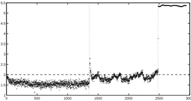
Fig. 12. Outlier analysis based on cointegration projection of training and testing data.
A final remark on Figure 12 concerns the spike above threshold at the interface between phases one and two (con-stant and varying temperature). At this point, the experiment was interrupted and modifications were made within the cham-ber; the question of whether cointegration failed at point is related to the question of whether this event should or should not be detected by an SHM algorithm; much more discussion on this point is given in [9].
E. Issues with Cointegration
Hopefully, the last section has convinced the reader that cointegration is a useful tool for the removal of confounding influences in SHM. However, use of the method requires some care. As a mathematical tool, certain conditions are required before cointegration can be applied with mathematical rigour;
appear to ‘effectively’ hold when one considers engineering problems [19]. Even so, recent work in SHM has unearthed circumstances where further thought is clearly needed. The remainder of this section will very briefly illustrate some issues which require clarification via further work.
1) Heteroskedasticity: Often, when engineers or physicists require stationarity, they will be satisfied with weak station-arity i.e. constancy with time of the mean and variance of a stochastic process. This condition at least allows one to apply some ideas from SPC to monitoring. If higher-order statistical moments are changing with time, it may be a challenge to define meaningful control limits or thresholds, but if the mean and variance are constant, one can use traditional ideas from SPC as guidance, if not with assured rigour. Unfortunately, weak stationarity does not seem to be as common as one would like; if the means of the signals of interest vary then there is the potential for cointegration to come to rescue, but what of time-varying variance? Although it is not a completely precise use of the term, the property of time-varying variance will be referred to here asheteroskedasticity[24]. The problem is that, if multiple moments of signals are nonstationary, one cannot rely on cointegration at least not the linear method -to provide a stationary residual. This will be illustrated via a case study. For reasons of space, the description will be very terse indeed, the reader is referred to [25] for more details.
The case study in question was concerned with monitor-ing the health of a (retired) footbridge at the UK National Physical Laboratory. The footbridge was intended to allow a comprehensive study of SHM using a wide variety of sensor modalities. The bridge was monitored in its normal undamaged condition over an extensive period covering a wide range of seasonal variations in its environment. Later in the monitoring campaign, systematic damage was introduced by overloading a cantilever portion of the bridge with a large weight. The authors of the current paper were interested in applying novelty detection in order to detect damage. However, the data considered was provided from a number of tilt sensors which proved extremely sensitive to the environmental conditions of the bridge. Figure 13 shows the response from one of the tilt sensors between January 2009 and February 2011; over this period, the bridge was not deliberately damaged, so the tilt signals could be used as training data for outlier analysis; however, the signal is clearly nonstationary in both the mean and variance.
Despite some concerns about the applicability of the ap-proach, in the absence of a better method, cointegration was applied to the data from seven tilt sensors in order to produce a residual for monitoring purposes. The results from cointegration are shown in Figure 14.
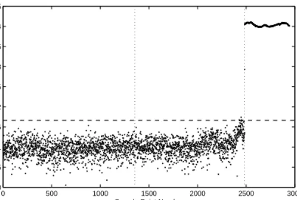
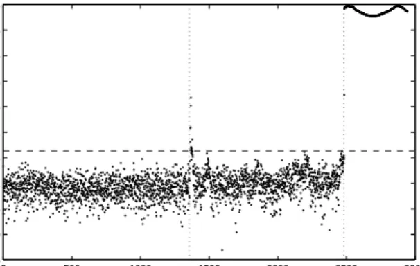
The figure requires a little explanation. The first vertical black line shows the end of the period of training data; this was taken as a full year in order to represent a full range of environmental conditions. The second vertical (blue) line shows the day on which deliberate damage was introduced via an overload; this means that the residual between the black and blue vertical lines is validation data for the structure in its (assumed) undamaged condition. (Further damage was
3 4 5 6 7 8 9 10 11 12 13 14 15 16 17 18 19 20 21 22 23 24 25 26 27 28 29 30 31 32 33 34 35 36 37 38 39 40 41 42 43 44 45 46 47 48 49 50 51 52 53 54 55 56 57 58 59 60
REVIEW COPY
Fig. 13. A tilt sensor signal from the NPL footbridge.Fig. 14. Cointegrated residual from the tilt sensor signals from the NPL footbridge.
introduced at later dates. The dates are indicated by vertical red lines in Figure 14; however, they are not relevant for the discussion here.) Measurements were taken from the tilt sensors on an hourly basis; however, the residuals plotted in Figure 14 are averaged over 24 measurements, yielding daily data. The averaging means that the figure shows, in SPC terms, an X-bar chart [7]. The horizontal dashed lines in the figure are the standard plus or minus three standard deviations control limits. The issue here is that the cointegrated residual is very clearly heteroskedastic; it retains structure showing seasonal changes in variance. Despite the obvious concerns about the validity of the control limits, the exercise appears to have been rather successful in the sense that the residual does not leave the control limits until after the deliberate damage was introduced; the speed that it does leave the limits is consistent with the timescale under which the cracks produced by the overload propagated and were found in visual inspections. The problem is that one cannot interpret the control limits
invalidated the assignment of 99.7% confidence to the region between the limits. This case study illustrates the issue of heteroskedasticy quite well and shows clearly that further research is needed. A cointegration theory is needed which can transform sets of heteroskedastic variables into (at least) weakly stationary residuals.
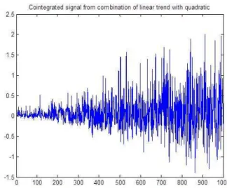
2) Nonlinearity: The second major issue with cointegration is that it is currently alineartheory. Although there have been attempts at generalisation, there is no completely satisfactory variant of the theory that can deal with the situation where a nonlinear transformation is needed in order to generate a stationary residual. A simple synthetic example which would cause problems for linear cointegration is given by the equa-tions,
xi = αti+ui
yi = βt2i +vi (10)
wherexi andyi are the sampled variables of interest, sharing
a deterministic dependence on timeti;ui andvi are assumed
to be independent Gaussian noise processes. The issue is that a nonlinear combination of the variables is needed in order to remove the explicit dependence onti. The combinationzi =
a1x2i +a2yi could be comparatively stationary if appropriate
parametersa1anda2could be found. This problem was posed
in [26] and a solution based on optimisation was proposed. In that paper, a differential evolution (DE) algorithm was used in order to determine a1 and a2 in such a way that some
measure of nonstationarity was minimised. The optimisation algorithm was successful in terms of finding good parameters; however, a close look at the cointegrated residual showed it to be heteroskedastic (Figure 15). The issue is clearly the result of the noise terms in equations (10); in fact, a simple calculation shows, zi = a1x2i +a2yi = a1(α 2 t2i + 2αtiui+u 2 i) +a2(βt 2 i +vi) (11)
Thus, even setting the a1 and a2 parameters to remove the
dominant t2
i terms, leaves a ‘noise’ component with linearly
increasing variance. The nonlinear cointegration scheme has thus produced a heteroskedastic residual, with all the issues that causes.
Nonlinearity also impacts on time series analysis in a slightly more subtle way. Many SPC-based algorithms assume that the monitored residuals have Gaussian distributions. If a structure or system is nonlinear, this Gaussian behaviour is not assured and the thresholds and alarm levels in X-charts etc. will be incorrectly estimated. One possible solution to this problem, which will not be discussed in detail here, is the use of Extreme Value Statistics (EVS) in order to compute thresholds [27].
III. SWITCHINGMODELS
The discussion now moves on to the issue of nonstationarity due to abrupt switching behaviour. As mentioned in the intro-duction, this section makes much more demands of the reader
3 4 5 6 7 8 9 10 11 12 13 14 15 16 17 18 19 20 21 22 23 24 25 26 27 28 29 30 31 32 33 34 35 36 37 38 39 40 41 42 43 44 45 46 47 48 49 50 51 52 53 54 55 56 57 58 59 60
REVIEW COPY
Fig. 15. Heteroskedastic residual from nonlinear cointegration algorithm.in terms of familiarity with ideas from Bayesian machine learning. It is hoped that, even without this familiarity, the main ideas will make themselves heard.
This section deals with a particular type of response sur-face switching model; the mixture of experts (MoE) model [28]. Details regarding the equations and derivations of the specific MoE model used here can be found in [29], and references therein. An MoE model is capable of automatically and probabilistically switching, via gates, between different regimes represented by experts. In the following sections, a Bayesian MoE model is introduced as a switching model in the context of SHM of the Z24 bridge: confounding influences are determined via a single environmental variable, temperature, which is required to be removed from the SHM feature dataset.
A. Bayesian Mixture of Experts
Letxi be adxdimensional input of the Z24 bridge at time
instant ti. Let the corresponding scalar output of interest be
yi, which for the case study used in this paper is given by
the second natural frequency of the bridge. A regression MoE model with M experts is,
yi= M X m=1
gm(xi, πm, θmg)fm(xi, wm) , (12)
where the mth expert is represented as a
linear-in-the-parameters vector function given byfm(xi, wm) = [xi1]wm,
where wm is a column vector representing the expert’s weights, and the 1 provides a bias term. The gating func-tion gm(xi, πm, θgm) is a normalised Gaussian function [30].
Each gate is parametrised by: the mean µ
m and the inverse
covariance Λm given byθg ={µ,Λ}={µm,Λm}Mm=1, and
the mixing coefficients π={πm}Mm=1 satisfyingπm≥0and
PM
m=1πm= 1. The bold notation in this section refers to sets
of parameters or multidimensional matrices.
as, p(yi|xi, π,θg,θe) = M X m=1 gm(x, πm, θmg)p(yi|xi, θme), (13)
where the probability distribution of themthexpert is a
Gaus-sian distribution, that is,p(yi|xi, θme) =N(yi|[xi1]wm, τ− 1
m ),
having meanfm and varianceτm−1.
The parameter vector for the experts consists of the weight vector W ={wm}M
m=1 and inverse variance τ ={τm}Mm=1,
given by θe = [W, τ]. Thus the set of unknown model
parameters is given by[π,θg,θe].
Given N i.i.d training samples are available such that X = [x1, . . . , xN]⊤, and y = [y1, . . . , yN]⊤, the
complete-data likelihood for the model is expressed as,
p(X, y, Z|π,θg,θe) = N Y i=1 M Y m=1 πmN(xi|µm,Λ− 1 m) N(yi|[xi 1]wm, τ− 1 m ) zim , (14)
where Z = {zim}M,Nm=1,i=1 are referred to as the latent
variables and they simplify the likelihood problem. If(xi, yi)
was generated from the mth expert then z
im = 1, or 0
otherwise.
B. Priors
Since the model is to be trained via Bayesian inference, priors are assigned to parameters of the gates and experts, except for the mixing coefficientsπwhich are treated as non-random variables. A Gaussian-Wishart prior is assigned to the gate parameters, p(µ,Λ) =p(µ|Λ)p(Λ) = M Y m=1 N(µ m|m0,(β0Λm) −1)W(Λ m|B0, ν0). (15) Similarly, the prior distribution of the joint weight and precision parameters of the experts is a Gaussian-Gamma distribution, p(W, τ|a) = M Y m=1 N(wm|0,(τmAm)−1)Ga(τm|ρ0, λ0), (16) where a = {am}M m=1, and am = [am,1. . . am,dx+1. A m is
a diagonal matrix containing the elements am. am,j is the
hyperparameter on which the expert weightwm,j depends and
it is assigned a Gamma distribution,
p(am,j) =Ga(am,j|c0, d0). (17)
Hence, the joint distribution of all the random variables conditioned on the mixing coefficients can be expressed hi-erarchically as, 3 4 5 6 7 8 9 10 11 12 13 14 15 16 17 18 19 20 21 22 23 24 25 26 27 28 29 30 31 32 33 34 35 36 37 38 39 40 41 42 43 44 45 46 47 48 49 50 51 52 53 54 55 56 57 58 59 60
REVIEW COPY
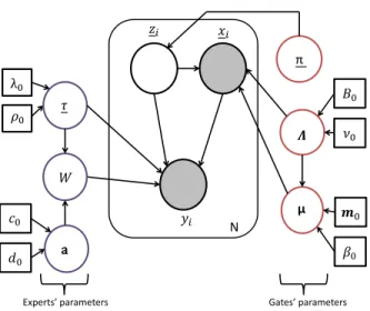
p(y, X, Z,µ,Λ,W, τ ,a|π) =p(X, y, Z|π,θg,θe)p(µ,Λ)p(W, τ|a)p(a), (18) shown as a graphical model in Figure (16).
N w
a
E G
Fig. 16. A graphical model for the Bayesian MoE model given in Equation (18). The plate denotes N i.i.d observations of observed variables xi and
yi(grey shading), and unobserved variableszi(no shading). The red circles
represent gate parameters while the purple circles represent expert parameters. The square boxes represent known parameters associated with the priors, given in Section III-B.
C. Variational Bayesian Inference
Bayesian inference involves finding a posterior distribution of the parameters of the modelp(θg,θe,a|y, π)according to
Bayes’ theorem,
p(θg,θe,a|y, π) =
p(y|X, π,θg,θe)p(θg,θe,a)
p(y|π) , (19)
where p(θg,θe,a) is the parameter prior distribution given
in Section III-B. An approximate Bayesian framework needs to be used to solve (19) since the marginal likelihood (or evidence) p(y|π) consists of a complex integral over the multidimensional parameter space. The choice of conjugate prior distributions, along with a latent variable model is elegantly accommodated by the variational Bayes expectation-maximisation (VBEM) framework [31]. The VBEM algorithm is an iterative process which updates approximate variational posterior distributions for the latent variables q(Z)and model parameters q(θg,θe,a) sequentially. Each variational
distri-bution update equation is determined by optimising the varia-tional lower bound ofp(y|π), and the update steps are stopped when this lower bound plateaus. The variational distributions of both the latent variables and the parameters for the MoE model described in this paper can be expressed in a factorised form as follows,
q(Z,µ,Λ, W, τ ,a) =q(Z)q(µ,Λ)q(W, τ)q(a). (20)
as the priors since conjugate priors were used in Section (III-B), and details of the expressions and derivations can be found in [29].
The mixing coefficients π of the gates are optimised us-ing maximum likelihood techniques: after every pass of the variational update equations the lower bound is maximised with respect to π, and hence π can be updated. Optimising the mixing coefficients of the gates in this way enables the number of experts to be set to a large number, and any mixing coefficient that converges to zero can be removed.
A posterior predictive distributionp(yN+1|xN+1,D), where
D = [y, X] and xN+1 is a new unseen input data point,
can be obtained once the VBEM algorithm has converged. In this case, the posterior predictive distribution is a Student-t distribution, and the meanE[yN+1]and variance var[yN+1]of
the predictions can be calculated.
D. Case Study: Z24 Bridge Data
The Z24 bridge is a well-studied bridge within the SHM community due to a year long comprehensive monitoring campaign [32]. The modal parameters of the structure were tracked, and environmental elements affecting the bridge, such as air temperature, were measured. Towards the end of the monitoring campaign a number of realistic damage events were introduced to the structure, and consequently SHM of the Z24 bridge was performed by various different groups, see [33], [34] among others.
In this work the features of interest are the temperature on the deck top and the second natural frequency of the bridge f2, which serve as the input and output of the modelling
process respectively. Figure 17 shows the time histories of these two variables, including the separate portions used for training (consists of temperature variation only) and testing (consists of both temperature variation and damage effect) the model. The vertical black line represents the point at which the different levels of damage were introduced to the bridge.
The second natural frequency exhibits nonstationarity due to large fluctuations in the dataset before the introduction of damage. The authors in [35] established a bilinear relationship between f2 and temperature using treed Gaussian processes
since the anomalous regions occurred during very cold periods when the bridge deck was frozen causing an increase in stiffness. This scenario demonstrates how damage sensitive parameters can also be susceptible to environmental variations. The VBEM-MoE algorithm was run 50 times due to the local maxima issue, and the model with the largest lower bound was chosen as being the model that best represents the data. The number of experts was set to 6 and any experts having πi < 10−5 were discarded. The results for the Z24
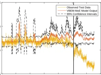
bridge data were obtained by training the MoE model using both temperature and its square as inputs to the model. The final model had 3 experts, with 2 splits occurring at 0.42◦C and 13.4◦C as shown by the black vertical lines in Figure 18. The red lines represent the mean of the predictions on the training data (blue), with 99%confidence intervals given by the dashed black lines. The algorithm is successful at identifying a switch
3 4 5 6 7 8 9 10 11 12 13 14 15 16 17 18 19 20 21 22 23 24 25 26 27 28 29 30 31 32 33 34 35 36 37 38 39 40 41 42 43 44 45 46 47 48 49 50 51 52 53 54 55 56 57 58 59 60
REVIEW COPY
Sampling Index 500 1000 1500 2000 2500 3000 3500 4000 4500 5000 Temperature ( °C) 0 20 40 Input Sampling Index 500 1000 1500 2000 2500 3000 3500 4000 4500 5000 f2 (Hz) 4.5 5 5.5 6 OutputFig. 17. The top plot shows the temperature variation on the deck top(input), while