DOI 10.1007/s10994-013-5365-4
Robust ordinal regression in preference learning
and ranking
Salvatore Corrente·Salvatore Greco· Miłosz Kadzi ´nski·Roman Słowi ´nski
Received: 7 January 2012 / Accepted: 19 April 2013 / Published online: 27 July 2013 © The Author(s) 2013. This article is published with open access at Springerlink.com
Abstract Multiple Criteria Decision Aiding (MCDA) offers a diversity of approaches de-signed for providing the decision maker (DM) with a recommendation concerning a set of alternatives (items, actions) evaluated from multiple points of view, called criteria. This paper aims at drawing attention of the Machine Learning (ML) community upon recent ad-vances in a representative MCDA methodology, called Robust Ordinal Regression (ROR). ROR learns by examples in order to rank a set of alternatives, thus considering a similar problem as Preference Learning (ML-PL) does. However, ROR implements the interactive preference construction paradigm, which should be perceived as a mutual learning of the model and the DM. The paper clarifies the specific interpretation of the concept of prefer-ence learning adopted in ROR and MCDA, comparing it to the usual concept of preferprefer-ence learning considered within ML. This comparison concerns a structure of the considered problem, types of admitted preference information, a character of the employed preference models, ways of exploiting them, and techniques to arrive at a final ranking.
Keywords Robust ordinal regression·Ranking·Preference learning·Multiple criteria decision aiding·Comparison·Preference modeling·Preference construction
Editors: Eyke Hüllermeier and Johannes Fürnkranz. S. Corrente·S. Greco
Department of Economics and Business, University of Catania, Corso Italia, 55, 95129 Catania, Italy S. Greco
Operations & Systems Management, University of Portsmouth, Portsmouth PO1 3DE, UK M. Kadzi´nski (
)·R. Słowi´nskiInstitute of Computing Science, Pozna´n University of Technology, 60-965 Pozna´n, Poland e-mail:milosz.kadzinski@cs.put.poznan.pl
R. Słowi´nski
1 Introduction
Ranking problems In ranking problems one aims at ordering a finite set of alternatives (items, actions) from the best to the worst, using a relative comparison approach. On the one hand, ranking problems have been of major practical interest in such various fields as economy, management, engineering, education, and environment (Zopounidis and Parada-los2010). For example, countries are ranked with respect to the quality of their information technology infrastructure, or established environmental policy goals, or level of introduced innovation. World-wide cities are rated on the basis of living conditions or human capital. When it comes to firms, they are ranked on the achieved level of business efficiency or relia-bility of being the best contractor for a particular project. Furthermore, magazines regularly publish rankings of MBA programs, schools, or universities.
On the other hand, a growing interest in ranking problems has recently emerged in fields related to information retrieval, Internet-related applications, or bio-informatics (see, e.g, Fürnkranz and Hüllermeier2011; Liu2011). Indeed, ranking is at the core of document retrieval, collaborative filtering, or computation advertising. In recommender systems, a ranked list of related items should be recommended to a user who has shown interest in some other items. In computational biology, one ranks candidate structures in protein struc-ture prediction problem, whereas in proteomics there is a need for the identification of fre-quent top scoring peptides.
The popularity of ranking problems encouraged researchers in different fields to propose scientific methods supporting the users in solving these problems. Remark that one has to dissociate problem formulation from problem solving because differences between the various approaches concern rather problem solving than problem formulation. The central point of these approaches concerns accounting for human preferences.
Multiple criteria decision aiding As far as Multiple Criteria Decision Aiding (MCDA) (Figueira et al.2005) is concerned, it offers a diversity of methods designed for structuring the decision problem and carrying forward its solution. An inherent feature of decision prob-lems handled by MCDA is a multiple criteria evaluation of alternatives (criteria = attributes with preference ordered scales). As multiple criteria are usually in conflict, the only objec-tive information that stems from the formulation of such a decision problem is a dominance relation (Pareto relation) in the set of alternatives. This relation leaves, in general, many alternatives incomparable, and thus one needs a method that would account for preferences of the decision maker (DM), making the alternatives more comparable. Thus, the DM is the main actor of the decision aiding process in whose name or for whom the decision aiding must be given. (S)he is usually assisted by an analyst who represents a facilitator of the process and needs to perform her/his role in the interaction with the DM.
MCDA is of essential help in preference elicitation, constructing a model of user’s pref-erences, and its subsequent exploitation which leads to a recommendation, e.g., a ranking of the considered alternatives. Thus, it is often defined as an activity of using some models which are appropriate for answering questions asked by stakeholders in a decision process (Roy2005). As noted by Stewart (2005), MCDA includes a comprehensive process involv-ing a rich interplay between human judgment, data analysis, and computational processes.
Dealing with DM’s preferences is at the core of MCDA. However, it is exceptional that facing a new decision problem, these preferences are well structured. Hence, the questions of an analyst and the use of dedicated methods should be oriented towards shaping these preferences. In fact, MCDA proceeds by progressively forming a conviction and commu-nicating about the foundations of these convictions. The models, procedures, and provided
results constitute a communication and reflection tool. Indeed, they allow the participants of the decision process to carry forward their process of thinking, to discover what is important for them, and to learn about their values. Such elements of responses obtained by the DMs contribute to recommending and justifying a decision, that increase the consistency between the evolution of the process and objectives and value systems of the stakeholders. Thus, de-cision aiding should be perceived as a constructive learning process, as opposed to machine discovery of an optimum of a pre-existing preference system or a truth that exists outside the involved stakeholders.
The above says that MCDA requires active participation of the stakeholders, which is often organized in an interactive process. In this process, phases of preference elicita-tion are interleaved with phases of computaelicita-tion of a recommended decision. Preference elicitation can be either direct or indirect. In case of direct elicitation, the DM is ex-pected to provide parameters related to a supposed form of the preference model. How-ever, a majority of recently developed MCDA methods (see, e.g., Ehrgott et al. 2010; Siskos and Grigoroudis2010), require the DM to provide preference information in an indi-rect way, in the form of decision examples. Such decision examples may either be provided by the DM on a set of real or hypothetical alternatives, or may come from observation of DM’s past decisions. Methods based on the indirect preference information are considered more user-friendly than approaches based on explicitly provided parameter values, because they require less cognitive effort from the DM at the stage of preference elicitation. More-over, since the former methods assess compatible instances of the preference model repro-ducing the provided decision examples, the DM can easily see what are the exact relations between the provided preference information and the final recommendation.
Robust ordinal regression One of the recent trends in MCDA concerning the develop-ment of preference models using examples of decisions is Robust Ordinal Regression (ROR) (Greco et al.2010). In ROR, the DM provides some judgments concerning selected alter-natives in the form of pairwise comparisons or rank-related requirements, expressed either holistically or with respect to particular criteria. This is the input data for the ordinal regres-sion that finds the whole set of value functions being able to reconstruct the judgments given as preference information by the DM. Such value functions are called compatible with the preference information. The reconstruction of the DM’s judgments by the ordinal regression in terms of compatible value functions is a preference learning step. The DM’s preference model resulting from this step can be used on any set of alternatives. Within the framework of ROR, the model aims to reconstruct as faithfully as possible the preference information of the DM, while the DM learns from the consequences of applying all compatible instances of the model on the set of alternatives.
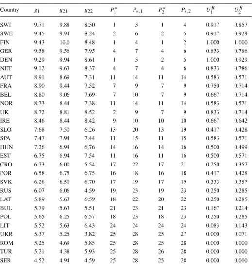
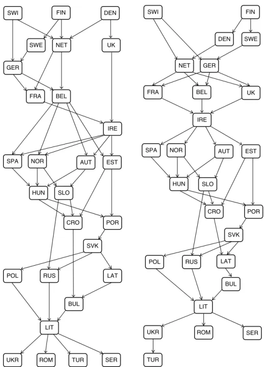
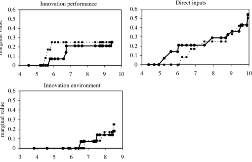
A typical application scenario of the ROR method is the following. Suppose a DM wants to rank countries with respect to their trend for innovation. Three criteria are used to eval-uate the countries: innovation performance, direct innovation inputs, and innovation envi-ronment. The DM is sure of some pairwise comparisons between countries which do not dominate each other. Moreover, (s)he claims that some countries should be placed in a spec-ified part of the ranking, e.g., at the bottom 5. This preference information is a starting point for the search of a preference model, which is a value function. If there is no instance of the preference model reproducing the provided holistic judgments, the DM could either decide to work with the inconsistency or revise some pieces of preference information impeding the incompatibility. Then, using ROR, i.e. solving a series of special optimization problems, one obtains two preference relation in the set of countries, called necessary and possible. While the first is true for all value functions compatible with the DM’s preference information, the
other is true for at least one such compatible value function. Moreover, ROR provides ex-treme ranks of particular countries and a representative compatible value function. Thanks to the analysis of the both outcomes of ROR at the current state of interaction as well as the form of the displayed representative preference model, the DM gains insights on her/his preferences. This stimulates reaction of the DM who may add a new or revise the old prefer-ence information. Such an interactive process ends when the necessary preferprefer-ence relation, extreme ranks, and/or a representative ranking yield a recommendation which, according to the DM, is decisive and convincing. This application example is developed in Sect.7.
Preference learning in machine learning When it comes to Machine Learning (ML), a “learning to rank” task is also involved with learning from examples, since it takes as an input a set of items for which preferences are known (Liu2011). Precisely, the training data is composed of lists of items with some partial order specified between items in each list. Preference Learning in ML (PL-ML) consists in discovering a model that predicts preference for a new set of items (or the input set of items considered in a different context) so that the produced ranking is “similar” in some sense to the order provided as the training data. In PL-ML, learning is traditionally achieved by minimizing an empirical estimate of an assumed loss function on rankings (Doumpos and Zopounidis2011).
Aim of the paper While there exist many meaningful connections and analogies between ROR-MCDA and PL-ML, there is also a series of noticeable differences concerning the process of learning a decision/prediction model from data. The aim of this paper is twofold. Firstly, we wish to draw attention of the ML community upon recent advances in ROR with respect to modeling DM’s preferences and interacting with her/him in the constructive learn-ing process. Our goal is to introduce ROR to specialists of PL in ML, so that they are aware of an alternative technique coming from a different field (MCDA), but aiming at learning preferences with respect to a similar problem. In fact, we review all previous developments in ROR, combining them under a unified decision support framework that permits to learn preferences by taking advantage of the synergy between different types of admitted pref-erence information and provided outcomes. Secondly, we compare philosophies of prefer-ence learning adapted in ROR and ML. In this way, we follow the preliminary comparisons between MCDA and ML made be Waegeman et al. (2009) and Doumpos and Zopounidis (2011). However, we focus the attention on ROR, which is closer to PL practiced in ML than many other MCDA methods, because it exploits preference information of similar type.
The contribution of the paper is methodological, and reference to PL-ML is at a philo-sophical level rather than at an experimental one. Note that an empirical comparison with respect to the output of ROR and PL-ML would not be meaningful, because there is no common context of their use and no objective truth is to be attained. Moreover, each method (ROR and PL-ML) is transforming the input preference information in a different way and introduces some instrumental bias in interactive steps, thus leading to different results. Fur-thermore, the concept of “learning” is implemented in different ways in PL-ML and in ROR. In ROR, learning concerns not only the preference model, but also the decision maker. Since the progress in learning of the DM is non-measurable, the experimental comparison of dif-ferent methods is ill-founded. Consequently, instead of providing an empirical comparison, our aim is rather to well explain and illustrate the steps of ROR.
Organization of the paper The remainder of the paper is organized as follows. In the next section, we present some basic concepts of ROR and MCDA. We also compare different as-pects of ranking problems and preference learning as considered in ROR and PL-ML. This
comparison is further continued throughout the paper with respect to the input preference in-formation, exploitation of the preferences, and evaluation of the provided recommendation. In particular, in Sect.3, we focus on different types of preference information admitted by the family of ROR methods. At the same time, we present the approach for learning of a set of compatible value functions. Section4describes the spectrum of procedures for robust-ness and sensitivity analysis that can be employed within the framework of ROR to support arriving at the final recommendation. In Sect.5, we put emphasis on the interactivity of the process of preference information specification. Section6reveals how ROR deals with in-consistency in the preference information provided by the DM. A case study illustrating the presented methodology is presented in Sect.7. The last section concludes the paper.
2 Basic concepts in MCDA and ROR and their comparison with preference learning in ML
2.1 Problem formulation
In the multiple criteria ranking problem, alternatives are to be ranked from the best to the worst. Precisely, the ranking of alternatives from setAresults from the ordering of indiffer-ence classes ofAwhich group alternatives deemed as indifferent (Roy2005).
Comparison: formulation of a ranking problem A ranking problem considered in MCDA corresponds most closely to an object ranking in PL-ML (see, e.g., Fürnkranz and Hüller-meier2011; Kamishima et al.2011), that aims at finding a model returning a ranking order among analyzed items. On the other hand, an instance ranking in PL-ML is about ordering a set of instances according to their (unknown) preference degrees (see, e.g., Waegeman and De Baets2011). This, in turn, is equivalent to a definition of a multiple criteria sorting problem (Zopounidis and Doumpos2002).
Let us formulate the problem that is considered in Robust Ordinal Regression (its detailed explanation is provided subsequently along with the comparative reference to PL-ML): Given:
– a finite set of alternativesA,
– a finite set of reference alternativesAR⊆A,
– a finite set of pairwise comparisons for some reference alternatives, expressed either holis-tically or with respect to a subset of criteria,
– a finite set of intensities of preference for some pairs of reference alternatives, expressed either holistically or with respect to a subset of criteria,
– a finite set of rank-related requirements for some reference alternatives, referring either to the range of allowed ranks or comprehensive values.
Find:
– a set of additive value functionsUARcompatible with the preference information provided
by the DM, i.e. value functions for which the pre-defined misranking error is equal to zero; each value functionU∈UARassumes as input a set of alternativesAand returns a
permutation (ranking) of this set,
– necessary and possible preference relations, for pairs or quadruples of alternatives inA, – extreme ranks and values for all alternatives inA,
– minimal sets of pieces of preference information underlying potential incompatibility of preference information.
Performance measure:
– margin of the misranking error comparing the provided pieces of preference information with the target ranking.
Technique:
– loop by interaction: analyze results provided in the previous iteration and supply prefer-ence information incrementally.
2.2 Data set
Generally, decision problems considered in MCDA involve a finite set A= {a1, a2, . . . ,
ai, . . . , an}ofnalternatives, i.e., objects of a decision, which are possible to be implemented
or have some interest within the decision aiding process.
Comparison: size of the data set Sets of alternatives in MCDA consist of modestly-sized collections of choices. In fact, multiple criteria ranking problems considered in Operations Research and Management Science (OR/MS) usually involve several dozens of alternatives (Wallenius et al.2008). Consequently, MCDA methods, including ROR, are designed to deal with the relatively small data sets, and the development of the computationally efficient algorithms that scale up well with the number of alternatives is not at the core of these approaches. On the other hand, real world applications of PL-ML often involve massive data sets (Waegeman et al. 2009). Typical ML applications are related to the Internet, in particular to recommender systems and information retrieval, and, thus, the scalability of the algorithms is a fundamental issue. Nevertheless, it is worth noting the complementarity of MCDA and ML from the viewpoint of the data size: the previous is more appropriate for several dozens of alternatives and over hundreds, the latter is more suitable.
Let us additionally note that in case of large data sets, it is very rare that the whole ranking is analyzed by the user. In fact, the rank of at most several dozens of alternatives is of interest to the DM, while the rest of the alternatives is neglected and, in fact, can remain unordered. Thus, to overcome the curse of dimensionality, in case of over hundreds of alternatives it might be useful first to filter out some significant subsets of alternatives, consisting of these less relevant to the DM. For this purpose, one may take advantage of some simple classification methods, or elimination by dominance (with the benchmarks in form of some artificial alternatives whose attractiveness should be evaluated directly by the DM). This would lead to limiting down the data set to several dozens relevant alternatives, which can be directly handled by ROR.
2.3 Data description
In MCDA, an important step concerns selection or construction of attributes describing the alternatives, based on the set of their elementary features. The aim is to obtain a consistent family ofmattributesG= {g1, g2, . . . , gj, . . . , gm}which permits a meaningful evaluation
and comparison of alternatives. Such attributes represent goals to be attained, objectives, impacts of considered alternatives, and points of view that need to be taken into account. In MCDA, one assumes that some values of attributes are more preferred than others, and thus, the corresponding value sets are transcoded into real-valued monotonic preference scales.
Such attributes are called criteria. Let us denote by Xj = {xj ∈R:gj(ai)=xj, ai∈A}
the set of all different evaluations on criteriongj,j∈J = {1,2, . . . , m}. We will assume,
without loss of generality, that the greatergj(ai), the better alternativeaion criteriongj, for
allj∈J.
Comparison: monotonicity of attributes/criteria In ROR (or, more generally, MCDA) one constructs criteria with explicit monotonic preference scales, whereas in ML the relation-ships between value sets of attributes and DM’s preferences (if any) are discovered from data for a direct use in classification or ranking. This means that in the majority of ML methods (e.g., approaches proposed in Chu and Ghahramani (2005a) and Herbrich et al. (1999), which solve the problem of ordinal regression), the monotonic preference scales converting attributes to criteria are neither used nor revealed explicitly.
Nevertheless, in the recent years, learning of predictive models that guarantee the mono-tonicity in the input variables has received increasing attention in ML (see, e.g., Feelders
2010; Tehrani et al.2012a). In fact, the difficulty of ensuring such monotonicity increases with the flexibility or nonlinearity of a model. In PL-ML, it is obtained either by a modifi-cation of learning algorithms or a modifimodifi-cation of the training data.
Apart from the monotonicity of criteria, the familyGconsidered in MCDA is supposed to satisfy another two conditions: completeness (all relevant criteria are considered) and non-redundancy (no superfluous criteria are taken into account). The set of attributes considered in ML, in general, does not have to satisfy such strict requirements.
Comparison: complexity of the considered alternatives/items As noted by Waegeman et al. (2009), ML is also concerned with more complex structures than alternatives described over a number of criteria. This includes, e.g., graphs in the prediction problems in bio-informatics or texts and images in the retrieval problems. Nevertheless, it is worth to note the recent effort of the MCDA community to apply decision aiding methods to geographical (spatial) data (Malczewski2010).
2.4 Preference/prediction model
The most straightforward way of ranking the alternatives in MCDA consists in aggregat-ing their individual performances on multiple criteria into a comprehensive (overall) perfor-mance. In particular, Multiple Attribute Utility Theory (MAUT) models the decision making situation with an overall value functionU (Keeney and Raiffa1976), and assigns a numer-ical score to each alternative. Such a score serves as an index used to decide the rank in a complete preorder. In ROR, in order to model the DM’s preference information, we use the additive value function:
U (a)= m j=1 uj gj(a) (1) where the marginal value functionsuj,j∈J, are monotone, non-decreasing and normalized
so that the additive value (1) is bounded within the interval[0,1]. Note that for simplicity of notation, one can writeuj(a),j∈J, instead ofuj(gj(a)). Consequently, the basic set of
constraints defining general additive value functions has the following form: uj(xjk)−uj(xj(k−1))≥0, k=2, . . . , nj(A), uj(xj1)=0, m j=1uj(x nj(A) j )=1, ⎫ ⎬ ⎭EA R BASE
wherex1
j, xj2, . . . , x nj(A)
j are the ordered values ofXj,xjk< x k+1
j ,k=1,2, . . . , nj(A)−1
(nj(A)= |Xj|andnj(A)≤n). General monotonic marginal value functions defined in this
way do not involve any arbitrary or restrictive parametrization. On the contrary, the majority of existing methods employ marginal value functions which are linear or piecewise linear (Siskos et al.2005). Note that piecewise linear functions require specification of the number of characteristic points which is not easy for most DMs.
Comparison: interpretability and regularization of the model The preference model in the form of an additive value function is appreciated by the MCDA community for both an easy interpretation of numerical scores of alternatives and a possibility of assessing relative importance of each evaluation on a particular criterion understood as its share in the compre-hensive value. Indeed, the interpretability and descriptive character of preference models is essential in MCDA, since it encourages the participation of the DM in the decision process. On the contrary, ML has mainly focused on the development of non-linear models, such as support vector machines (SVMs) (see, e.g., Herbrich et al.2000; Joachims2002) or neural networks. The higher predicting ability and possibility of capturing complex interdependen-cies by such models results, however, in less confidence in their employment by the users who need to interpret and understand the underlying process (Waegeman et al.2009).
Note that in a regression learning problem in ML, the task of finding the utility function corresponds just to learning an appropriate mapping from data to real numbers. Thus, the utility function is used in a rather instrumental way, and the model is not deeply analyzed by the user in order to gain insights on the character of the alternatives.
The researchers in ML indicate also the need for the regularization, which takes into account the trade-offs between complexity and performance of the model, preventing over-fitting on the data (Waegeman et al.2009). In MCDA the focus is put on the explicative char-acter of the employed models, rather than statistically predictive PL. Thus, MCDA models do not involve regularization, being, however, vulnerable to noise.
2.5 Input data
A preference elicitation process in MCDA consists in an interaction between the DM and the analyst, and leads the DM to express information on her/his preferences within the frame-work of the assumed preference model. Such information is materialized by a set of plausible values of the parameters related to the formulation of the model. At the end of the decision aiding process, the use of a preference model for the inferred parameters should lead to a result which is compatible with the DM’s preferential system.
In case of an additive value function, some MCDA methods require the DM to provide constraints on the range of weights of linear marginal value functions, or on the range of variation of piecewise linear marginal value functions. The DM may have, however, diffi-culties to analyze the link between a specific value function and the resulting ranking. Thus, ROR implements the preference disaggregation analysis, which is a general methodological framework for the development of a decision model using examples of decision made by the DM. In fact, ROR admits and enhances the variety of indirect preference information concerning the set of reference alternativesAR= {a∗, b∗, . . .}(usually,AR⊆A).
This information may have the form of pairwise comparisons of reference alternatives stating the truth or falsity of the weak preference relation (Greco et al.2008). Such a com-parison may be related to the holistic evaluation of alternatives on all considered criteria or on a subset of criteria considered in a hierarchical structure (Corrente et al.2012). In the same spirit, the DM may provide holistic or partial comparisons of intensities of preference
between some pairs of reference alternatives (Figueira et al.2009). Furthermore, (s)he is admitted to refer to the range of allowed ranks that a particular alternative should attain, or to constraints on the final value scores of the alternatives. In this way, the DM may rate a given alternative individually, at the same time collating it with all the remaining alternatives (Kadzi´nski et al.2013a). Finally, ROR accounts for the preference information regarding in-teractions betweenn-tuples (e.g., pairs or triples) of criteria (see, e.g., Greco et al.2013).
ROR methods are intended to be used interactively, with an increasing subset of reference alternatives and a progressive statement of holistic judgments. The DM may assign gradual confidence levels to pieces of preference information provided in the subsequent iterations (Greco et al.2008; Kadzi´nski et al.2013a).
The paradigm of learning from examples which is implemented in ML is a counterpart approach to preference modeling and decision aiding (Fürnkranz and Hüllermeier2010). Traditional machine learning of preferences was motivated by the applications where de-cision examples come from observation of people’s behavior rather than from direct ques-tioning. For example, typical ML applications are related to the Internet, in particular to recommender systems and information retrieval. In the previous, the task is to recommend to the user a new item (like movie or book) that fits her/his preferences. The recommenda-tion is computed on the base of the learning informarecommenda-tion describing the past behavior of the user. In the latter, the task is to sort (or rank) the documents retrieved by the search engine according to the user’s preferences. Nevertheless, recently in PL-ML one also develops the procedures which require direct human assessment (Liu2011). For example, in information retrieval, one uses pooling methods whose role is to collect documents that are more likely to be relevant. Considering the query, human annotators specify whether a document is rel-evant or not, or whether a document is more relrel-evant than the other, or they provide the total order of the documents.
Comparison: inferring a faithful model Both ROR and PL-ML aim at inferring a (prefer-ence or prediction) model that permits to work out a final recommendation (e.g., a ranking of alternatives) being concordant with a value system of the DM; thus, both of them deal with the same decision problem.
Comparison: learning of a model from examples Both ROR and PL-ML try to build a DM’s preference model from decision examples (exemplary judgments) provided by the DM—in ML decision examples form a training data set, while in ROR, preference infor-mation; thus, both of them comply with the paradigm of learning by example. In both ap-proaches learning concerns the model, because one integrates into it the expressed/collected preferences.
Comparison: amount of the available human preferences The number of decision exam-ples forming the training set or the preference information is quite different in ML and ROR: while the first is big enough for statistical learning, the second is usually limited to small sets of items, which excludes statistical analysis.
Comparison: preference elicitation for the utility functions Preference elicitation can be perceived as one of the main links between decision analysis and PL-ML. An extensive survey on the utility elicitation techniques is presented in Braziunas and Boutilier (2008). The authors classify the elicitation methods in different ways. For example, they distinguish the local and global queries. The previous involve querying only single attributes or small subsets of attributes, whereas the latter concern the comparison of the complete outcomes over all attributes. ROR takes advantage of both types of techniques.
As for the representation of uncertainty over user preferences, two main approaches have been proposed. On the one hand, in a Bayesian approach, uncertainty over utilities is quan-tified probabilistically (see, e.g., Braziunas and Boutilier 2005). On the other hand, in a feasible set uncertainty, the space of feasible utilities is defined by some constraints on the parameters of the user’s utility function (this approach is also called Imprecisely Specified Muti-Attribute Utility Theory (ISMAUT) (see, e.g., White et al.1983). ROR represents the latter approach.
2.6 Performance measure
Disaggregation analysis in MCDA aims at constructing a preference model that represents the actual decisions made by the DM as consistently as possible. To measure the perfor-mance of this process, ROR considers a margin of the misranking on a deterministic pref-erence information. When the margin is not greater than zero, this means that for a given preference information, no compatible value function exists. This is considered as a learning failure. Subsequently, the DM could either decide to work with the inconsistency (agreeing that some of the provided pieces would not be reproduced by the inferred model) or re-move/revise some pieces of preference information impeding the incompatibility. In fact, in ROR the application of the learned preference model on the considered set of alternatives makes greater sense when there is no inconsistency, and misranking error is reduced to zero (i.e. the margin of the misranking error is greater than zero).
On the other hand, in ML the predictive performance of a ranker is measured by a loss function. Indeed, any distance or correlation measure on rankings can be used for that pur-pose (Fürnkranz and Hüllermeier2010). When it comes to the inconsistencies in training data, PL-ML treats it as noise and hard cases that are difficult to learn.
Comparison: minimization of a learning error Both ROR and ML try to represent pref-erence information with a minimal error—ML considers a loss function, and ROR a mis-ranking error. In this way, both of them measure the distance between the DM’s preferences and the recommendation which can be obtained for the assumed model. However, the loss function considered in ML is a statistical measure of the performance of preference learning on an unknown probabilistic distribution of preference information, whereas a margin of the misranking error is a non-statistical measure.
Obviously, it is possible to optimize the error considered in ROR within a standard ML setting. Nevertheless, such an optimization is not conducted, because it would lead to select a single instance of the preference model. Instead, our aim is to work with all instances of the preference model for which the value of the margin of the misranking error is greater than the acceptable minimal threshold (i.e., zero in case the inconsistency is not tolerated). That is why, in ROR we analyze the mathematical constraints on the parameters of the constructed preference model to which the preference information of the DM was converted. Precisely, the preference relations in the whole set of alternatives result from solving some mathematical programming problems with the above constraints.
Comparison: dealing with inconsistencies ROR treats inconsistencies explicitly during construction of the preference model. In this case, the DM may either intentionally want to pursue the analysis with the incompatibility or (s)he may wish to identify its reasons with the use of some dedicated procedures, which indicate the minimal subsets of troublesome pieces of preference information. As emphasized in Sect.6, analysis of such subsets is in-formative for the DM and it permits her/him to understand the conflicting aspects of her/his statements.
PL-ML methods process noise in the training data in a statistical way. In fact, the ML community perceives the noise-free applications as uncommon in practice and the way of tolerating the inconsistencies is at the core of ML methods.
Let us additionally note that the noise-free ROR is well adapted to handing preferences of a single DM. There are several studies (e.g. Pirlot et al.2010) proving great flexibility of general value functions in representing preference information of the DM. Consequently, if preferences of the DM do not violate dominance and are not contradictory, it is very likely that they could be reproduced by the model used in ROR. Nevertheless, ROR has been also adapted to group decision (Greco et al.2012; Kadzi´nski et al.2013b).
2.7 Ranking results
In case of MCDA methods using a preference model in form of a value function, tra-ditionally, only one specific compatible function or a small subset of these functions has been used to determine the final ranking (see, e.g., Beuthe and Scannella 2001; Jacquet-Lagrèze and Siskos1982). To avoid such arbitrary limitation of the instances under-lying the provided recommendation and to prevent the DMs from an embarassing selection of some compatible instances, which requires interpretation of their form, ROR (Greco et al.
2010) postulates taking into account the whole set of value functions compatible with the provided indirect preference information. Then, the recommendation for the set of alterna-tives is worked out with respect to all these compatible instances.
When considering the set of compatible value functions, the rankings which can be ob-tained for them can vary substantially. To examine how different can those rankings be, ROR conducts diverse sensitivity and robustness analysis. In particular, one considers two weak preference relations, necessary and possible (Greco et al.2008). Whether for an ordered pair of alternatives there is necessary or possible preference depends on the truth of preference relation for all or at least one compatible value function, respectively. Obviously, one could reason in terms of the necessary and the possible, taking into account only a subset of cri-teria or a hierarchical structure of the set of cricri-teria (Corrente et al.2012). In this case, the presented results are appropriately adapted to reflect the specificity of a particular decision making situation.
However, looking at the final ranking, the DM is usually interested in the position which is taken by a given alternative. Thus, one determines the best and the worst attained ranks for each alternative (Kadzi´nski et al.2012a). In this way, one is able to assess its position in an overall ranking, and not only in terms of pairwise comparisons. Finally, to extend original ROR methods in their capacity of explaining the necessary, possible and extreme results, one can select a representative value function (Kadzi´nski et al. 2012b). Such a function is expected to produce a robust recommendation with respect to the non-univocal prefer-ence model stemming from the input preferprefer-ence information. Precisely, the representative preference model is built on the outcomes of ROR. It emphasizes the advantage of some al-ternatives over the others when all compatible value functions acknowledge this advantage, and reduces the ambiguity in the statement of such an advantage, otherwise.
Comparison: considering the plurality of compatible models In traditional ML rank loss minimization leads to a choice of a single instance of the predictive model. This corresponds to the traditional UTA-like procedures in MCDA, which select a “mean”, “central”,“the most discriminant”, or “optimal” value function (see Beuthe and Scannella2001; Despotis et al.
Nevertheless, in PL-ML one can also indicate some approaches that account for the plu-rality of compatible instances. For example, Yaman et al. (2011) present a learning algo-rithm that explicitly maintains the version space, i.e., the attribute-orders compatible with all pairwise preferences seen so far. However, since enumerating all Lexicographic Prefer-ence Models (LPMs) consistent with a set of observations can be exponential in the number of attributes, they rather sample the set of consistent LMPs. Predictions are derived based on the votes of the consistent models; precisely, given two objects, the one supported by the majority of votes is preferred. When comparing with a greedy algorithm that produce the “best guess” lexicographic preference model, the voting algorithm proves to be better when the data is noise-free.
Furthermore, Viappiani and Boutilier (2010) present a Bayesian approach to adaptive utility selection. The system’s uncertainty is reflected in a distribution, or beliefs, over the space of possible utility functions. This distribution is conditioned by information acquired from the user, i.e. (s)he is asked questions about her preference and the answers to these queries result in updated beliefs. Thus, when an inference is conducted, the system takes into account multiple models, which are, however, weighted by their degree of compatibility.
Comparison: generalization to the new users/stakeholders The essence of the decision aiding process is to help a particular DM in making decision with respect to her/his pref-erences. In fact, ROR is precisely addressed to a given user and the generalization to other users is neither performed nor even desired. On the contrary, in some applications of PL-ML, the aim is to infer the preferential system of a new user on the basis of preferences of other users.
2.8 Interaction
ROR does not consider the DM’s preference model as a pre-existing entity that needs to be discovered. Instead, it assumes that the preference model has to be built in course of an interaction between the DM and the method that translates preference information provided by the DM into preference relations in the set of alternatives. ROR encourages the DM to reflect on some exemplary judgments concerning reference alternatives. Initially, these judgments are only partially defined in the DM’s mind. The preferences concerning the alternatives are not simply revealed nor they follow any algorithm coming from the DM’s memory. Instead the DM constructs her/his judgments on the spot when needed. This is concordant with both the constructivist approach postulated in MCDA (Roy 2010b) and the principle of posterior rationality postulated by March (1978). The provided preference information contributes to the definition of the preference model. In ROR, the preference model imposes the preference relations in the whole set of alternatives.
In this way, ROR emphasizes the discovery of DM’s intentions as an interpretation of actions rather than as a priori position. Analyzing the obtained preference relations, the DM can judge whether the suggested recommendation is convincing and decisive enough, and whether (s)he is satisfied with the correspondence between the output of the preference model and the preferences that (s)he has at the moment. If so, the interactive process stops. Otherwise, the DM should pursue the exchange of preference information. In particular, (s)he may enrich the preference information by providing additional exemplary judgments. Alternatively, if (s)he changed her/his mind or discovered that the expressed judgments were inconsistent with some previous judgments that (s)he considers more important, (s)he may backtrack to one of the previous iterations and continue from this point. In this way, the process of preference construction is either continued or restarted.
The use of the preference model shapes the DM’s preferences and makes her/his con-victions evolve. As noted by Roy (2010b), the co-constructed model serves as a tool for looking more thoroughly into the subject, by exploring, reasoning, interpreting, debating, testing scenarios, or even arguing. The DM is forced to confront her/his value system with the results of applying the inferred model on the set of alternatives. This confrontation leads the DM to gaining insights on her/his preferences, providing reactions in the subsequent it-eration, as well as to better understanding of the employed method. In a way, ROR provokes the DM to make some partial decisions that lead to a final recommendation. The method presents its results so that to invite the DM to an interaction—indeed, comparing the nec-essary and possible relations, the DM is encouraged to supply preference information that is missing in the necessary relation. Let us emphasize that the knowledge produced during the constructive learning process does not aim to help the DM discover a good approximate decision that would objectively be one of the best given by her/his value system. In fact, the “true” numerical values of the preference model parameters do not exist, and thus it is not possible to refer directly to the estimation paradigm. Instead, the DM is provided with a set of results derived from applying some working assumptions and different reasoning modes, and it is the course of the interactive procedure that enhances the trust of the DM in the final recommendation.
Comparison: preference construction in ROR vs. preference discovery in typical ML In fact, ROR can be qualified as preference construction method, whereas the typical meth-ods of ML can be named as preference discovery. The main differences between the two approaches are the following:
– preference construction is subjective while preference discovery is objective: within pref-erence construction, the same results can be obtained (i.e., accepted, rejected, doubted, etc.) in a different way by different DMs, while within preference discovery, there is no space for taking into account the reactions of the DM;
– preference construction is interactive while preference discovery is automatic: the DM actively participates in the process of preference construction, while in the preference discovery the DM is asked to give only some preference information that are transformed in a final result by the adopted methodology without any further intervention of the DM; – preference construction provides recommendations while preference discovery gives
pre-dictions: the results of a preference construction give to the DM some arguments for making a decision, while the results of preference discovery give a prevision of what will be some decisions;
– preference construction is DM-oriented while preference discovery is model-oriented: preference construction aims the DM learns something about her/his preferences, while preference discovery assumes the model would learn something about the preferences of the DM.
In the view of above remarks, let us emphasize that preference learning in MCDA does not only mean statistical learning of preference patterns, i.e. discovery of statistically validated preference patterns. MCDA proposes a constructivist perspective of preference learning in which the DM takes part actively.
Comparison: recommendation vs. elicitation The main objective of the majority of PL-ML methods is to exploit current preferences and to assess a preference model applicable on the set of alternatives in a way that guarantees the satisfying concordance between the discovered/predicted results and the observed preferences. Thus, PL-ML is focused rather
on working out a recommendation, being less sensitive to gaining explanation of the results. On the other hand, the role of preference elicitation within ROR is to acquire enough knowl-edge and arguments for explanation of the decision. This enables the DM to establish the preferences that previously had not pre-existed in her/his mind, to accept the recommenda-tion, and to appropriately use it (and possibly share with the others). ROR (or, generally, “preference construction”) is a mutual learning of the model and the DM to assess and un-derstand preferences on the considered set of alternatives.
Nevertheless, this issue has been also considered in PL-ML especially with respect to the setting of recommender systems and product search. In fact, there are several works that advocate for eliciting user preferences, suggesting an incremental and interactive user sys-tem. Although the context of their use and the feedback presented to the user is significantly different than in ROR, they can be classified as “preference construction” as well.
For example, Pu and Chen (2008) formulate a set of interaction design guidelines which help users state complete and sound preferences with recommended examples. They also describe strategies to help users resolve conflicting preferences and perform trade-off deci-sions. These techniques allow gaining a better understanding of the available options and the recommended products through explanation interfaces.
Moreover, there are also noticeable advances in the active learning, which deals with the algorithms that are able to interactively query the user to obtain the desired outputs for new items (Settles2012). In particular, in Viappiani and Boutilier (2010) one presents Bayesian approaches to utility elicitation that involve an interactive preference elicitation in order to learn to make optimal recommendation to the user. The system is equipped with an active learning component which is employed to find relevant preference queries that are asked to the user. Similar task has been considered, e.g., in Radlinski and Joachims (2007) and Tian and Lease (2011). These studies report that active exploration strategy substantially outperforms passive observation and random exploration, and quickly leads to a presentation of the improved ranking to a user.
Comparison: user interface vs. truly interactive process Obviously, an interaction with the user in the PL-ML methods that have not considered this aspect can be modeled with the use of an interface accounting for user preferences. However, in our understanding a truly interactive process requires exploitation of the learned models, delivering to the user con-sequences of such exploitation, and encouraging her/him to the further involvement. Note that the feedback that can be provided by the majority of PL-ML methods is formed by the results predicted by the single optimized model. The user can then react by reinforcing or neglecting some parts of the outcome. Nevertheless, such a feedback is rather poor, because it does not guide the user through the process. Moreover, since PL-ML setting admits noise, there is no guarantee that the provided preferences will be integrated into the model in the subsequent iteration. On the other hand, noise-free ROR reveals the possible, necessary, ex-treme, and representative consequences of the preference information provided at the current stage of interaction. In this way, it leads the DM to have a better understanding of her/his preferences and invites her/him to a deeper exploitation of the preference model.
Comparison: analyst vs. user interface Let us also note that real-world MCDA problems involve an analyst, who interacts with the DM in order to guide the process. Once the analyst enters into the interaction with the DM, (s)he becomes a co-constructor of the knowledge produced; thus, (s)he cannot be perceived as being outside the decision aiding process. It is difficult to imagine that a software interface can play the same role.
Comparison: validation of the results In MCDA it is assumed that the analyst cooperates with the DM and the quality of the model is validated by an interactive process during which (s)he judges the correspondence between the output of the preference model and one’s preferential system. On the other hand, the generalizing ability of the model is the core issue in the validation stage of all statistical learning models. In PL-ML the validation stage involves, e.g., additional testing sets or the use of resampling methods.
2.9 Features of preference learning in robust ordinal regression
Belton et al. (2008) consider some important features of a preference learning process within MCDA. Let us recall them, pointing out how they are extant in ROR:
– flexibility of the interactive procedure, which is related to the capacity of incorporating any preference information coming from the DM: ROR admits the DM to provide a wide spectrum of indirect preference information; note that flexibility can be decomposed in generality, reversibility and zooming capacity;
– generality of the preference model, which is related to the universality and the plurality of the decision model: for the features of plurality of instances and universality of value functions in ROR, there is a large credit for generality;
– universality of the preference model, which considers the non-specificity of the form of the value function, in the sense that the less specific the form, the greater the chance that the model learns in a sequence of iterations: the additive value function with monotone marginal value functions considered within ROR constitutes a very general preference model and consequently it reaches a very good level of universality, which is far more universal than the model admitting only linear marginal value functions;
– plurality of instances of value functions which regards consideration of only one, sev-eral, or even all compatible instances of the considered preference model: ROR takes into account the whole set of additive value functions compatible with the preference informa-tion provided by the DM, which is evidently more plural than considering only one value function as in the traditional approaches;
– reversibility which is understood as the possibility for the DM to return to a previous iteration of interaction with the method: ROR permits in any moment to retract, to modify or to remove the already expressed pieces of preference information;
– zooming which regards the possibility to represent preferences in a limited zone of the evaluation spaces of considered criteria: ROR enables to add preference information rela-tive to alternarela-tives from a particular region of the evaluation space of considered criteria, which results in a more precise representation of preferences in this local region.
3 Preference information
In this section, we present a variety of preference information admitted by the family of ROR methods designed for dealing with multiple criteria ranking problems. The wide spectrum of the accounted types of preference information guarantees the flexibility of the interac-tive procedure. We discuss the usefulness of each accounted type of preference information, and we present mathematical models which are able to reproduce preferences of the DM, i.e. translate the exemplary decisions of the DM into parameters of the value function. The constraints related to every new piece of preference information can reduce the feasible polyhedron of all compatible value functions. Let us denote the holistic set of constraints obtained in this way byEAR
the provided preference information byUAR. Although the considered set of additive value
functions composed of marginal monotone value functions already ensures a large credit for generality, plurality, and universality, we extend the basic model by accounting for interac-tions between criteria.
Comparison: variety of preference information admitted by the method ROR admits the variety of indirect preference information concerning the set of reference alternatives. This means that the DM can use pairwise comparisons or rank-related requirements or magni-tudes of preference if (s)he feels comfortable with this kind of information and (s)he is able to provide it for the problem at hand. However, (s)he is not obliged to specify preference in-formation of each type. On the contrary, ML methods consider rather preference inin-formation of a given type and the user has to express her/his preferences in the precise form required by the employed approach (e.g., solely pairwise comparisons or only the magnitudes of preference).
3.1 Pairwise comparisons
Comparing alternatives in a pairwise fashion, which is admitted by numerous decision-theoretic methods, is consistent with intuitive reasoning of DMs, and requires from the DM relatively small cognitive effort (Fürnkranz and Hüllermeier2010). In the UTAGMSmethod
(Greco et al.2008), which initiated the stream of further developments in ROR, the ranking of reference alternatives does not need be complete as in the original UTA method (Jacquet-Lagrèze and Siskos1982). Instead, the DM may provide pairwise comparisons just for those reference alternatives (s)he really wants to compare. Precisely, the DM is expected to pro-vide a partial preorderonARsuch that, fora∗, b∗∈AR, a∗b∗meansa∗is at least as
good asb∗.
Obviously, one may also refer to the relations of strict preferenceor indifference∼, which are defined as, respectively, the asymmetric and symmetric part of. The transition from a reference preorder to a value function is done in the following way: fora∗, b∗∈AR,
U (a∗)≥U (b∗)+ε, ifa∗b∗, U (a∗)=U (b∗), ifa∗∼b∗, E
AR GMS
whereεis a (generally small) positive value.
Comparison: use of pairwise comparisons in PL-ML Learning by pairwise comparisons paradigm is a ML counterpart of MCDA. Thus, the rankers in ML require exemplary pair-wise preferences of the forma∗b∗ suggesting thata∗should be ranked higher thanb∗. Then, the algorithm needs to care about preserving the relative order between the compared pairs of items. Such decomposition of the original problem into a set of presumably simpler subproblems is not only advantageous for human decision making, but it is also useful from a ML point of view (Fürnkranz and Hüllermeier2010). It is the case, because the resulting learning problem (i.e. operating on every two items under investigation and minimizing the number of misranked pairs) can typically be solved in a more accurate and efficient way. In PL-ML, one has proposed several algorithms, whose major differences are in the loss function. Let us mention a few of them.
Fürnkranz and Hüllermeier (2010) discuss various standard loss functions on ranking that can be minimized in expectation. In particular, they consider the expected Spearman rank correlation between the true and the predicted ranking, or the number of pairwise inversions,
i.e., Kendall’s tau, which is traditionally considered in the UTA-like methods. Furthermore, RankBoost (Freund et al.2003) formalizes learning to rank as a problem of binary classifica-tion on instance pairs. By adopting the boosting approach, it trains one weak ranker at each iteration. After each round, the item pairs are re-weighted in order to relatively increase the weight of wrongly ranked pairs. In fact, RankBoost minimizes the exponential loss. When it comes to the model of Ranking SVM (Joachims2002), it uses representation of the ex-amples as points in space, which carry the rank information. These labeled points are used to find a boundary that specifies the order of the considered points. Precisely, Ranking SVM employs the loss function in the form of a hinge loss defined on item pairs. Finally, instead of explicitly defining the loss function, LambdaRank (Burges et al.2006) directly defines the gradient. The authors note that it is easier to specify rules determining how to change the rank order of documents than to construct a smooth loss function. Some improvements of the “learning to rank” algorithms that enable better ranking performance consist in empha-sizing likely top-ranked items and balancing the distribution of items pairs across queries (Liu2011).
3.2 Intensities of preference
In some decision making situations the DMs are willing to provide more information than a partial preorder on a set of reference alternatives, such as “a∗is preferred tob∗ at least as much asc∗is preferred tod∗”. The information related to the intensity of preference is accounted by the GRIP method (Figueira et al.2009). It may refer to the comprehensive comparison of pairs of reference alternatives on all criteria or to a particular criterion only. Precisely, in the previous case, the DM may provide a partial preorder ∗ onAR×AR,
whose meaning is: fora∗, b∗, c∗, d∗∈AR,
a∗, b∗∗c∗, d∗⇔a∗is preferred tob∗at least as much as c∗is preferred tod∗.
When referring to a particular criteriongj,j∈J, rather than to all criteria jointly, the
mean-ing of the expected partial preorder∗jonAR×ARis the following: fora∗, b∗, c∗, d∗∈AR,
a∗, b∗∗jc∗, d∗⇔a∗is preferred tob∗at least as much as c∗is preferred tod∗on criteriongj.
In both cases, the DM is allowed to refer to the strict preference and indifference relations rather than to weak preference only. The transition from the partial preorder expressing intensity of preference to a value function is the following: fora∗, b∗, c∗, d∗∈AR,
U (a∗)−U (b∗)≥U (c∗)−U (d∗)+ε, if(a∗, b∗)∗(c∗, d∗), U (a∗)−U (b∗)=U (c∗)−U (d∗), if(a∗, b∗)∼∗(c∗, d∗), uj(a∗)−uj(b∗)≥uj(c∗)−uj(d∗)+ε, if(a∗, b∗)∗j(c∗, d∗)forgj∈G, uj(a∗)−uj(b∗)=uj(c∗)−uj(d∗), if(a∗, b∗)∼∗j(c∗, d∗)forgj∈G, ⎫ ⎪ ⎪ ⎪ ⎪ ⎪ ⎪ ⎪ ⎪ ⎪ ⎪ ⎪ ⎬ ⎪ ⎪ ⎪ ⎪ ⎪ ⎪ ⎪ ⎪ ⎪ ⎪ ⎪ ⎭ EGRI PAR
Comparison: use of intensities/magnitudes of preference in PL-ML When using the pref-erence information in the form of pairwise comparisons, one loses the granularity in the relevance judgments (any two items with different relevance/attractiveness degrees can con-struct an item pair). Thus, several algorithms have been proposed in PL-ML to tackle the problem of considering the magnitude of preference. In particular, Qin et al. (2007) sug-gested the use of leveraged multiple hyperplanes to preserve the magnitude of rating differ-ences on the basis of the Ranking SVM algorithm and demonstrated the importance of pref-erence magnitude. Further, Cortes et al. (2007) analyzed the stability bounds of magnitude preserving loss functions for generalization error. They proposed two magnitude-preserving ranking algorithms, MPRank and SVRank, with reports of the improvement on mis-ordering loss. Finally, in the MPBoost method (Zhu et al.2009) one applies the preference magnitude into the exponential loss function of boosting to improve the accuracy of ranking.
Note that introducing a quaternary relation∗, ROR considers the intensity of preference in an ordinal way. On the contrary, in PL-ML it is supposed that there exists a cardinal rating such that the magnitude of preference is a monotonic function of difference between the cardinal ratings. Moreover, in ROR the intensity of preference can be referred also to a single criterion, while this option has not been yet considered in PL-ML.
3.3 Rank-related requirements
When looking at the final ranking, the DM is mainly interested in the position which is attained by a given alternative and, possibly, in its comprehensive score. Therefore, in the RUTA method (Kadzi´nski et al.2013a), the kind of preference information that may be sup-plied by the DM have been extended by information referring to the desired rank of reference alternatives, i.e. final positions and/or scores of these alternatives. In fact, when employing preference disaggregation methods in the context of sorting problems in MCDA (instance ranking in PL-ML), the DM is allowed to refer to the desired final assignment (label) of the reference alternatives. In this perspective, it was even more justified to adapt similar idea to multiple criteria ranking problems, and to allow DMs expressing their preferences in terms of the desired ranks of reference alternatives.
In fact, people are used to refer to the desired ranks of the alternatives in their judgments. In many real-world decision situations (e.g., evaluation of candidates for some position) they use statements such asa∗should be among the 5 % of best/worst alternatives, orb∗should be ranked in the second ten of alternatives, orc∗is predisposed to secure the place between 4 and 10. These statements refer to the range of allowed ranks that a particular alternative should attain. When using such expressions, people do not confront “one vs one” as in pairwise comparisons or “pair vs pair” as in statements concerning intensity of preference, but rather rate a given alternative individually, at the same time somehow collating it with all the remaining alternatives jointly.
Moreover, specification of the desired ranks of the alternatives addresses one of the com-monly encountered disadvantages of using traditional UTA-like methods. On the one hand, very often all reference alternatives or their significant subsets are grouped together in the upper, or middle, or lower part of the ranking. As a result, the positions of reference alter-natives in the final ranking are very close to each other. On the other hand, some UTA-like procedures (Beuthe and Scannella2001) allow discrimination of the comprehensive values of reference alternatives. This usually results in the uniform distribution of their positions in the final ranking, e.g., one alternative is placed at the very top, the other just in the middle, and the third one at the very bottom. If the rankings obtained in the two above described scenarios are inconsistent with the DM’s expectations, accounting for the rank-related re-quirements may be used as a tool to prevent such situations. It is the case, since the ranks
specified by the DM may be interpreted in terms of the desired “parts” of the final ranking in which reference alternatives should be placed.
Finally, there is a correspondence between the input in form of rank-related requirements and the output presented as the extreme ranks (see Sect.4.2). Consequently, the presentation of the extreme ranks may constitute a good support for generating reactions from the part of the DM, who may incrementally supply rank-related requirements.
Let us denote the range of desired ranks for a particular reference alternative a∗∈A provided by the DM with[PDM∗ (a∗), P∗,DM(a∗)]. The constraints referring to the desired
values of some reference alternatives may be expressed as follows: Ua∗∈U∗,DM
a∗, UDM∗ a∗,
where U∗,DM(a∗)≤UDM∗ (a∗) are precise values from the range [0,1] that are provided
by the DM. Formally, these requirements are translated into the following constraints: for a∗∈AR U (a∗)−U (b)+M·v> a∗,b≥ε, for allb∈A\ {a∗} b∈A\{a∗}va>∗,b≤P∗,DM(a∗)−1 U (b)−U (a∗)+M·va<∗,b≥ε, for allb∈A\ {a∗} b∈A\{a∗}va<∗,b≤n−PDM∗ (a∗) va>∗,b+v < a∗,b≤1, for allb∈A\ {a∗} ⎫ ⎪ ⎪ ⎪ ⎪ ⎪ ⎪ ⎪ ⎪ ⎪ ⎪ ⎪ ⎪ ⎪ ⎪ ⎪ ⎪ ⎬ ⎪ ⎪ ⎪ ⎪ ⎪ ⎪ ⎪ ⎪ ⎪ ⎪ ⎪ ⎪ ⎪ ⎪ ⎪ ⎪ ⎭ ifa∗⇒PDM∗ a∗, P∗,DM a∗, U (a∗)≥U∗,DM(a∗) U (a∗)≤UDM∗ (a∗) ifU a∗∈U∗,DM a∗, UDM∗ a∗, ⎫ ⎪ ⎪ ⎪ ⎪ ⎪ ⎪ ⎪ ⎪ ⎪ ⎪ ⎪ ⎪ ⎪ ⎪ ⎪ ⎪ ⎪ ⎪ ⎪ ⎪ ⎪ ⎪ ⎪ ⎬ ⎪ ⎪ ⎪ ⎪ ⎪ ⎪ ⎪ ⎪ ⎪ ⎪ ⎪ ⎪ ⎪ ⎪ ⎪ ⎪ ⎪ ⎪ ⎪ ⎪ ⎪ ⎪ ⎪ ⎭ EARU T AR
whereM is an auxiliary variable equal to a big positive value,v>
a∗,b and v<a∗,b are binary
variables associated with comparison of a∗ to alternativeb. Using these binary variables, the above set of constraints guarantees that there are at mostP∗,DM(a∗)−1 alternatives
which are ranked better thana∗, and at most n−PDM∗ (a∗)alternatives which are ranked worse thana∗.
Comparison: use of rank-related requirements in PL-ML Rank-related requirements con-cerning positions of the alternative have not been yet considered as an input information in PL-ML. Nevertheless, some algorithms (see, e.g., Rudin2009; Usunier et al.2009) do con-sider the positions of items in the final ranking. Precisely, since top positions are important for users, the focus is put on the top-ranked items by punishing the errors occurring in the head of the ranking. Moreover, the direct feedback in form of exemplary utility degrees is admitted by several PL-ML methods.
3.4 Hierarchy of criteria
Complex real-world decision problems, such as choosing a new product pricing strategy, deciding where to locate manufactoring plants, or forecasting the future of a country, involve
factors of different nature. These factors may be political, economic, cultural, environmental, technological, or managerial. Obviously, it is difficult for the DMs to consider so different points of view simultaneously when assessing the quality of the alternatives.
By applying a hierarchical structure, such complex decision problems can be decom-posed into a hierarchy of more easily comprehended sub-problems, each of which can be analyzed independently (Saaty2005). It is the matter of fact that a hierarchy is an efficient way to organize complex systems, being efficient both structurally, for representing a sys-tem, and functionally, for controlling and passing information down the system. Once the hierarchy is built, the DMs may first judge the alternatives and then receive feedback about them, with respect to their impact on a particular element in the hierarchy.
In fact, practical applications are often explicitly imposing a hierarchical structure of cri-teria. For example, in economic ranking, alternatives may be evaluated on indicators which aggregate evaluations on several sub-indicators, and these sub-indicators may aggregate an-other set of sub-indicators, etc. In this case, the marginal value functions may refer to all levels of the hierarchy, representing values of particular scores of the alternatives on in-dicators, sub-inin-dicators, sub-sub-inin-dicators, etc. In order to treat this case, we extend the previously introduced notation:
– lis the number of levels in the hierarchy of criteria, – Gis the set of all criteria at all considered levels,
– IGis the set of indices of particular criteria representing position of criteria in the hierar-chy,
– mis the number of the first level criteria,G1, . . . , Gm,
– Gr∈G, with r=(i1, . . . , ih)∈IG, denotes a subcriterion of the first level criterionGi1 at
levelh; the first level criteria are denoted byGi1,i1=1, . . . , m,
– n(r)is the number of subcriteria ofGrin the subsequent level, i.e. the direct subcriteria
ofGrareG(r,1), . . . , G(r,n(r)),
– gt:A→R, with t=(i1, . . . , il)∈IG, denotes an elementary subcriterion of the first level
criterionGi1, i.e a criterion at levellof the hierarchy tree ofGi1,
– ELis the set of indices of all elementary subcriteria:
EL=t=(i1, . . . , il)∈IG where ⎧ ⎪ ⎪ ⎨ ⎪ ⎪ ⎩ i1=1, . . . , m, i2=1, . . . , n(i1), . . . il=1, . . . , n(i1, . . . , il−1)
– E(Gr)is the set of indices of elementary subcriteria descending fromGr, i.e.
E(Gr)= (r, ih+1, . . . , il)∈IG where ⎧ ⎨ ⎩ ih+1=1, . . . , n(r), . . . il=1, . . . , n(r, ih+1, . . . , il−1)
thus,E(Gr)⊆EL.
In case of hierarchy of criteria, the DM may provide a partial preorderronARor a partial
preorder ∗r onAR×AR, which should be interpreted analogously as pairwise
compar-isons or statements regarding the intensity of preference, however, limited only to a crite-rion/subcriterionGr. In this context, the value function of an alternativea∈Awith respect
to criterion/subcriterionGris: Ur(a)= t∈E(Gr) ut gt(a) .