Multi-objective optimisation using the Bees Algorithm

Ca r d i f f

U N I V E R S I T Y P R I F Y S C O L

CA'RDVg)

Multi-Objective Optimisation

using the Bees Algorithm

A thesis submitted to Cardiff University in candidature for the degree of

Doctor of Philosophy

by

Ji Young Lee, B.Eng., M. Eng.

Manufacturing Engineering Centre School of Engineering

Cardiff University United Kingdom

UMI Number: U585417

All rights reserved

INFORMATION TO ALL USERS

The quality of this reproduction is dependent upon the quality of the copy submitted.

In the unlikely event that the author did not send a complete manuscript and there are missing pages, these will be noted. Also, if material had to be removed,

a note will indicate the deletion.

Dissertation Publishing

UMI U585417

Published by ProQuest LLC 2013. Copyright in the Dissertation held by the Author. Microform Edition © ProQuest LLC.

All rights reserved. This work is protected against unauthorized copying under Title 17, United States Code.

ProQuest LLC

789 East Eisenhower Parkway P.O. Box 1346

ABSTRACT

In the real world, there are many problems requiring the best solution to satisfy numerous objectives and therefore a need for suitable Multi-Objective Optimisation methods.

Various Multi-Objective solvers have been developed recently. The classical method is easily implemented but requires repetitive program runs and does not generate a true “Pareto” optimal set. Intelligent methods are increasingly employed, especially population-based optimisation methods to generate the Pareto front in a single run.

The Bees Algorithm is a newly developed population-based optimisation algorithm which has been verified in many fields. However, it is limited to solving single optimisation problems. To apply the Bees Algorithm to a Multi- Objective Optimisation Problem, either the problem is converted to single objective optimisation or the Bees Algorithm modified to function as a Multi- Objective solver.

To make a problem into a single objective one, the weighted sum method is employed. However, due to failings of this classical method, a new approach is developed to generate a true Pareto front by a single run.

This work also introduces an enhanced Bees Algorithm. A new dynamic selection procedure improves the Bees Algorithm by reducing the number o f parameters and new neighbourhood search methods are adopted to optimise the Pareto front.

The enhanced algorithm has been tested on Multi-Objective benchmark functions and the classical Environmental/Economic power Dispatch Problem (EEDP). The results obtained compare well with those produced by other population- based algorithms.

Due to recent trends in renewable energy systems, it is necessary to have a new model of the EEDP. Therefore, the EEDP was amended in conjunction with the Bees Algorithm to identify the best design in terms o f energy performance and carbon emission reduction by adopting zero and low carbon technologies. This computer-based tool supports the decision making process in the design of a Low-Carbon City.

ACKNOWLEDGEMENTS

I would like to thank my supervisor Professor Due Truong Pham for his excellent supervision, continuous encouragement and support. He deserves more thanks than I can express for the amount o f time he gave me, and for making that time the most rewarding hours o f my academic life.

I would also like to thank the members and staff o f the MEC, especially Dr

Michael Packianather and Celia Rees for their support throughout my research work. My thanks are also due to all my Cardiff Bay Bees colleagues, especially Dr Marco Castellani and Dr Ahmed Haj Darwish, who contributed to my work through their valuable help, advice and technical support.

Furthermore, special thanks also go to Professor Jin-Seok Oh and the members of the E2E Lab. at Korea Maritime University for their support. I also want to thank Dr Jae-Min Kim and Roger Judd for their valuable help.

Finally, I reserve my deepest gratitude for my parents, Sang-Min Lee and Mi-Ok Oh who gave and have given me continuous support and encouragement throughout my studies. Many thanks also to my sisters Mi-Jung Lee and Hey-Jung Lee, my brother Neung-Hui Lee and special thanks goes to my sister Sun-Young Lee.

DECLARATION

This work has not previously been accepted in substance for any degree and is not concurrently submitted in candidature for any degree.

S i g n e a ^ T ^ T T S r r r ? ^ . .... ( Ji Young Lee ) Date. f.'. l . ' . t i . ?!. °

Statement 1

This thesis is being submitted in partial fulfilment o f the requirements for the degree o f PhD.

Signed . . ( Ji Young Lee) Date.

Statement 2

This thesis is the result of my own independent work/investigations, except where otherwise stated. Other sources are acknowledged by explicit references. A bibliography is appended.

Signed ... . ( Ji Young Lee ) D ate.. .^t! / / .?:/ . ^P. L°

Statement 3

I hereby give consent for my thesis, if accepted, to be available for photocopying and for inter-library loan, and for the title and summary to be made available to outside organisations.

i l I

2

i

/ ( i

/

2oio

CONTENTS

LIST OF TABLES... xvi

ABBREVIATIONS... xix

NOMENCLATURE... xxiii

1 INTRODUCTION...1

1.1 Motivation...1

1.2 Research Aim and Objectives... 3

1.3 Outline of the Thesis... 5

2 MULTI-OBJECTIVE OPTIMISATION USING SWARM-BASED OPTIMISATION ALGORITHMS... 7

2.1 Multi-Objective Optimisation (M O O )... 7

2.2 Multi-Objective solvers... 10

2.2.1 Classical m ethods...10

2.2.1.1 Weighted sum method... 13

2.2.2 Intelligent m ethods...14

2.2.2.1 Population-based Multi-Objective solvers... 14

2.2.2.1.1 Genetic Algorithms (G A s)... 17

2.2.2.1.2 Ant algorithm...26

2.2.2.1.3 Particle Swarm Optimisation (PSO )...31

2.2.2.1.4 Artificial Immune System (AIS)... 36

2.2.2.1.5 Bacteria Foraging Optimisation Algorithm (BFOA) 41 2.2.2.1.6 Bee-inspired Algorithms... 45

2.3 Sum m ary... 58

3 THE PARETO-BASED BEES ALGORITHM WITH MEMORISED SOLUTIONS FOR MULTI-OBJECTIVE PROBLEMS... 59

3.1 Prelim inaries... 59

3.2 Applications... 60

3.2.1 The Environmental/Economic Dispatch Problem (EED P) 60 3.2.1.1 Objective functions...64

3.2.1.2 Constraints... 65

3.2.1.3 Multi-Objective form ulation...65

3.2.1.4 System parameters... 66

3.2.2 Benchmark mathematical Multi-Objective functions...66

3.3 The Pareto-based Bees Algorithm with memorised solutions... 69

3.4 Results... 73

3.4.1 Results o f the EE D P... 73

3.4.1.1 Comparison o f Multi-Objective Optimisation Algorithm s. 74 3.4.1.2 Effect o f patch size... 81

3.4.1.3 Effect o f number o f memorised solutions... 85

3.4.1.4 Comparison of the number o f solutions and Pareto fronts...88

3.5 Sum m ary...98

4 AN ENHANCED BEES ALGORITHM FOR MULTI-OBJECTIVE PROBLEMS...99

4.1 Prelim inaries... 99

4.2 Applications...100

4.2.1 The Environmental/Economic Dispatch Problem (EED P) 100 4.2.2 Benchmark mathematical Multi-Objective functions... 100

4.3 An enhanced Bees Algorithm for solving Multi-Objective Optimisation Problems... 109

4.3.1 Enhancements... 109

4.3.1.1 Global enhancem ents...109

4.3.1.2 Local enhancem ents...110

4.3.1.2.1 Basic neighbourhood search (basicNGH) method 111 4.3.1.2.2 Random and weighted sum neighbourhood search (randomNGH and wsNGH) methods...115

4.3.2 The proposed algorithm s...119

4.3.2.1 The Single-Cycled Bees Algorithm (SC B A )...119

4.3.2.2 The Multi-Cycled Bees Algorithm (M C BA )...122

4.4 Results...125

4.4.1 Results of the EED P... 125

4.4.1.1 Comparison o f two extreme Pareto solutions... 128

4.4.1.1.1 Comparison o f Multi-Objective Optimisation Algorithms...128

4.4.1.1.2 Effect o f neighbourhood search m ethods... 140

4.4.1.1.3 Effect o f settings...145

4.4.1.3 Comparison between WSBA-w and MCBA-wsNGH

methods... 162

4.4.2 Results o f benchmark mathematical functions... 167

4.5 Sum m ary...175

5 OPTIMISATION OF MULTI-FUEL ENERGY SYSTEMS FOR A LOW-CARBON CITY USING THE BEES ALGORITHM ... 177

5.1 Prelim inaries... 177

5.2 The proposed system m odel...183

5.3 Proposed techniques...189

5.3.1 The Simultaneous Technique (ST)... 189

5.3.2 The Sequential Technique with Multi-Optimisation (STMO)...197

5.3.2.1 Equations for the Pareto ® fro n t... 198

5.3.2.2 Equations for the Pareto ® fro n t...202

5.3.3 The Sequential Technique with Single Optimisation (STSO)... 203

5.3.4 System parameters...204

5.4 Results...209

5.4.1 Comparison of two extreme solutions... 209

5.4.1.1 Effects o f techniques...212

5.4.1.1.1 S e ttin g l... 212

5.4.1.1.2 Setting2... 213

5.4.1.2 Effect of settings...213

5.4.2 Comparison of Pareto fronts...218

5.4.3 Additional comparisons... 232

6 CONCLUSION... 239

6.1 Contributions... 239

6.2 Conclusions...240

6.3 Suggestions for future research... 242

APPEN DIX...243

REFERENCES...268

LIST OF FIGURES

Figure 2.1 Illustration of the Pareto concept for a bi-objective optimisation

problem...11

Figure 2.2 Taxonomy o f Multi-Objective solvers... 12

Figure 2.3 Pareto front generation using population-based techniques...16

Figure 2.4 Simplified flowchart o f a Genetic Algorithm ...19

Figure 2.5 Genetic Algorithm for Multi-Objective Optimisation Problems...21

Figure 2.6 Flowchart o f Ant Colony Optimisation algorithm...30

Figure 2.7 Simplified flowchart o f Particle Swarm Optimisation algorithm... 33

Figure 2.8 Pseudo code o f Immune System model (fitness scoring)...39

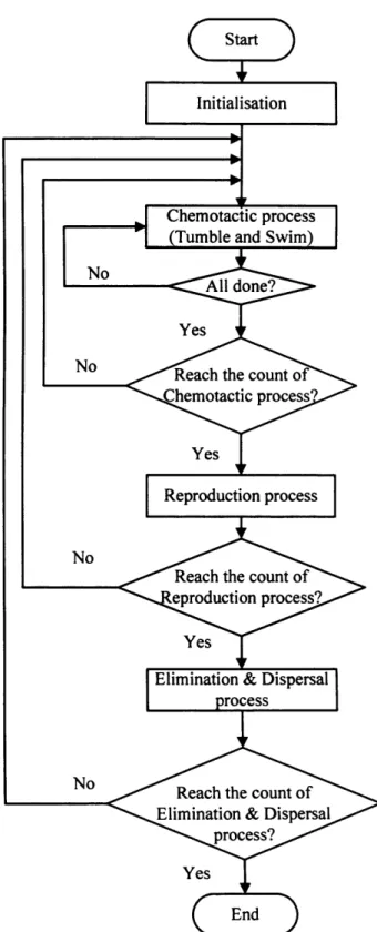
Figure 2.9 Simplified flowchart o f Bacterial Foraging Optimisation Algorithm 44 Figure 2.10 Bee behaviour and algorithm s...47

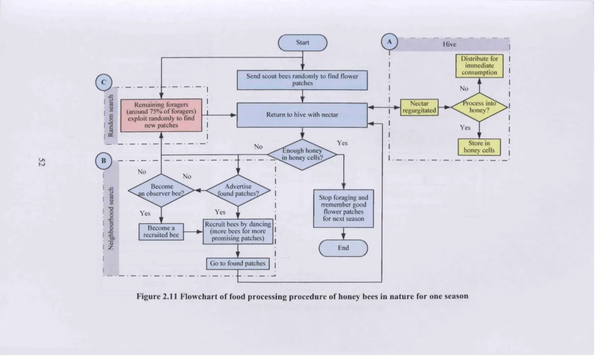
Figure 2.11 Flowchart of food processing procedure o f honey bees in nature for one season... 52

Figure 2.12 Flowchart o f the Bees Algorithm... 53

Figure 3.1 Single-line diagram o f IEEE 30-bus test system ...63

Figure 3.2 Illustration o f the concept for the Bees Algorithm with memorised solutions... 71

Figure 3.3 Flowchart of the proposed Pareto-based Bees Algorithm with memorised solutions...72

Figure 3.5 The results by WSBA(20)...95

Figure 3.6 The Pareto fronts by W SBA -e(20)... 96

Figure 3.7 The Pareto fronts by W SBA -w (20)... 97

Figure 4.1 Flowchart for the basicNGH m ethod... 113

Figure 4.2 The concept o f basicNGH method...114

Figure 4.3 The concept for the both randomNGH and wsNGH methods 117 Figure 4.4 The flowchart for the both randomNGH and wsNGH m ethods 118 Figure 4.5 The flowchart of the Single-Cycled Bees Algorithm (SC B A ) 121 Figure 4.6 The concept o f the Multi-Cycled Bees Algorithm (M CBA ) 123 Figure 4.7 The flowchart o f the Multi-Cycled Bees Algorithm (M C BA ) 124 Figure 4.8 Box plot of the best cost (fc) regarding neighbourhood search methods ... 141

Figure 4.9 Box plot of the best emissions (fe) regarding neighbourhood search m ethods... 143

Figure 4.10 Box plot o f the best cost (fc) regarding settings...148

Figure 4.11 Box plot o f the best emission (fe) regarding settings... 149

Figure 4.12 Box plots of the number of evaluations...154

Figure 4.13 Box plots of program running tim es... 156

Figure 4.14 Box plots o f the number o f Pareto solutions... 158

Figure 4.15 Pareto fronts regarding neighbourhood search methods... 160

Figure 4.17 Box plots of the best cost between the WSBA-m(22) and the

MCBA-wsNGH... 164

Figure 4.18 Comparison between the WSBA-/w(22) and the MCBA-wsNGH 165 Figure 4.19 Comparison of the Pareto fronts between the WSBA-w(22) (or m-Pareto(22)) and the MCBA-wsNGH...166

Figure 4.20 Pareto fronts of convex functions without constraints... 171

Figure 4.21 Pareto front o f non-convex function without constraints...172

Figure 4.22 Pareto front of three-objective function without constraints 172 Figure 4.23 Pareto fronts o f functions with constraints...173

Figure 4.24 Comparison of Pareto fronts between the WSBA-m(20) (or m-Pareto(20)) and the SCBA-randomNGH... 174

Figure 5.1 Outline plan for ASAN new to w n ...186

Figure 5.2 Overview o f the procedure for this w ork... 187

Figure 5.3 Multi-fuel energy system configuration... 188

Figure 5.4 System structure of Simultaneous Technique (S T )... 191

Figure 5.5 Flowchart of the Simultaneous Technique (ST) using the Bees A lgorithm ... 192

Figure 5.6 Structure o f the Sequential Technique with Multi-Optimisation (STM O )... 199

Figure 5.7 Concept of the Sequential Technique with Multi-Optimisation (STM O )... 200

Figure 5.8 Flowchart o f the Sequential Technique with Multi-Optimisation (STMO) using the Bees A lgorithm ...201 Figure 5.9 Structure of the Sequential Technique with Single Optimisation (STSO)... 205 Figure 5.10 Concept o f the Sequential Technique with Single Optimisation (STSO)... 206 Figure 5.11 Flowchart o f the Sequential Technique with Single Optimisation (STSO) using the Bees Algorithm...207 Figure 5.12 Box plot o f the best cost (fc) regarding techniques in setting2 216 Figure 5.13 Pareto fronts o f the Simultaneous Technique (ST)... 220 Figure 5.14 Individual proportions o f the energy system and CO2 reduction (%) with the Simultaneous Technique (ST) s e ttin g l... 221 Figure 5.15 Individual proportions o f the energy system and CO2 reduction (%) with the Simultaneous Technique (ST) setting2... 222 Figure 5.16 Pareto fronts of the Sequential Technique with Multi-Optimisation (STM O )...223 Figure 5.17 Individual proportions o f the energy system and CO2 reduction (%) with the STMO se ttin g l...224 Figure 5.18 Individual proportions o f the energy system and CO2 reduction (%) with the STMO setting2... 225 Figure 5.19 Pareto fronts of Sequential Technique with the Single Optimisation (STSO)... 226

Figure 5.20 Individual proportions o f the energy system and CO2 reduction (%) with the STSO settingl... 227 Figure 5.21 Individual proportions o f the energy system and CO2 reduction (%) with the STSO setting2... 228 Figure 5.22 Comparison o f Pareto fronts of three techniques in settin g l 229 Figure 5.23 Individual proportions o f the energy system with three techniques

...230 Figure 5.24 Comparison o f Pareto fronts between the ST and partial Pareto front o f thermal systems which exceeds electrical dem and... 231 Figure 5.25 Box plots of results with settingl... 235 Figure 5.26 Box plots of results with setting2... 236

LIST OF TABLES

Table 2.1 Applications o f the Bees Algorithm... 48 Table 3.1 Coefficients for the test system ...67 Table 3.2 Equations for Multi-Objective mathematical function optimisation... 68 Table 3.3 Parameters for the Environmental/Economic Dispatch Problem 75 Table 3.4 Test settings... 76 Table 3.5 Symbols used in Table 3.6 to 3 .1 2 ...78 Table 3.6 Comparison of results between MOPSO and the proposed Bees Algorithm for finding the best fuel cost (fc) ...79 Table 3.7 Comparison of results between MOPSO and the proposed Bees

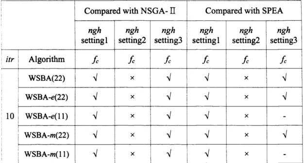
Algorithm for finding the best NOx emissions (fe)... 80 Table 3.8 Comparison of results between NSGA- I I , SPEA and the proposed Bees Algorithms (/7r=10) for the best cost (fc) ... 82 Table 3.9 Comparison of results regarding neighbourhood size for the best cost ( f c )...83 Table 3.10 Comparison o f results regarding neighbourhood size for the best emissions (fe)... 84

Table 3.11 Comparison o f results regarding memorised solutions for the best cost

( f c)...86

Table 3.12 Comparison results regarding memorised solutions for the best

emissions (fe)... 87

Table 3.13 The average number o f solutions for each 20 independent runs 89 Table 3.14 Parameters o f the Bees Algorithm for benchmark mathematical functions...93

Table 3.15 Results for benchmark mathematical functions...94

Table 4.1 Convex functions without constraints... 104

Table 4.2 Non-con vex functions without constraints... 105

Table 4.3 Functions with constraints... 107

Table 4.4 Three-functions optim isation...108

Table 4.5 Parameter settings for the basicNGH and the SCBA-randomNGH...126

Table 4.6 Parameter settings for the SCBA-wsNGH and the MCBA-wsNGH 127 Table 4.7 Comparison between the SCBA-basicNGH, the SCBA-randomNGH and M O PSO ...130

Table 4.8 Comparison between the SCBA-basicNGH, the SCBA-randomNGH a n d N S G A -n ...131

Table 4.9 Comparison between the SCBA-basicNGH, the SCBA-randomNGH and S P E A ... 133

Table 4.10 Comparison between the SCBA-wsNGH and MOPSO... 134

Table 4.11 Comparison between the SCBA-wsNGH, the MSBA-wsNGH and M O PSO ... 135

Table 4.12 Comparison between NSGA- I I , SPEA and the SCBA-wsNGH ... 138

Table 4.13 Comparison between NSGA- I I , SPEA, the SCBA-wsNGH and the MSBA-wsNGH... 139

Table 4.14 The result of statistic analyses regarding settings by SPSS... 147

Table 4.15 The average number o f evaluations, program running times and number o f Pareto solutions...153

Table 4.16 The result o f statistical analyse o f two extreme Pareto solutions ... 164

Table 4.17 Parameters for the Bees Algorithm ...168

Table 4.18 The result o f the number o f evaluation and Pareto solutions 169 Table 5.1 Peak demands and total roof areas...188

Table 5.2 Limit o f each system ...195

Table 5.3 Parameters o f the proposed multi-fuel energy system ... 208

Table 5.4 Parameter setting for the Bees Algorithm ... 210

Table 5.5 The average o f two extreme solutions from 10 independent runs .... 211

Table 5.6 Statistical result in s e ttin g l... 214

Table 5.7 Statistical results in setting2... 215

Table 5.8 Statistical result from t- te s tregarding setting...217

Table 5.9 The average values from 10 independent program ru n s...234

ABBREVIATIONS

Artificial Bee Colony algorithm

Autonomous Bee Colony Optimisation algorithm Ant Colony Optimisation

Artificial Intelligence Artificial Immune System Adaptive Inertia Weight Factor Analysis o f variance

Automated Red Teaming The Ant System

The Adaptive Weighted-Sum method The Bees Algorithm

The Bees Algorithm-assisted Multi objective Optimisation Problems

Bacterial Chemotaxis Multi-Objective Optimisation Algorithm

Bee Colony Optimization algorithm Bacteria Foraging Optimisation Algorithm Bees System

Bee Swarm Optimisation Combined Heat and Power Chaotic Local Search Carbon dioxide

Coefficient O f Performance Decision Maker

Evolutionary Algorithm/Evolutionary Algorithms

EDAS Entropy-based Density Assessment Scheme EEDP The Environmental/Economic Dispatch Problem EMOIA Evolutionary Multi-Objective Immune Algorithm EMOO Evolutionary Multi-Objective Optimisation ESRU Energy Systems Research Unit

FACTS Flexible AC Transmission System devices FCM Fuzzy C-Means clustering

FON Fonseca and Fleming’s study

GA/GAs Genetic Algorithm/Genetic Algorithms HBF Honey Bee Foraging algorithm

HBMO Honey-Bees Mating Optimisation algorithm IEEE Institute of Electrical and Electronics Engineers

KRW Korea currency (won)

KUR Kursawe’s study

MACS Multiple Ant Colony System MBA Multiobjective Bees Algorithm MBO

MCBA-wsNGH

Marriage Process in Honey Bees algorithm

The Multi-Cycled Bees Algorithm with weighted sum neighbourhood search method

MG Micro-Grid

MIMO MC- Multiple Input Multiple Output Multi Carrier Code Division CDMA Multiple Access system

MO Multi-Objective

MOAIS Multi-Objective Artificial Immune System MOBA The Multi-Objective Bees Algorithm MOBCO

MODEST

Multi-Objective Bee Colony Optimisation algorithm Model for Optimisation o f Dynamic Energy System with Time-Dependent Components and Boundary Conditions

Multi-Objective Evolutionary Algorithm/Multi-Objective MOEA/MOEAS

Evolutionary Algorithms

e -MOEA e -Multi-Objective Evolutionary Algorithm MOGA Multi-Objective Genetic Algorithm

MOO Multi-Objective Optimisation

Multi-Objective Optimisation Problem/Multi-Objective MOOP/MOOPs

Optimisation Problems

MOPSO Multi-Objective Particle Swarm Optimisation NPGA Niched-Pareto Genetic Algorithm

NOx Generic term for mono-nitrogen oxides (NO and NO2) NSGA Non-dominated Sorting Genetic Algorithm

N SG A -13 Non-dominated Sorting Genetic Algorithm- II PACO Population-based Ant Colony Optimisation PAES Pareto Archived Evolution Strategy algorithm PCB Printed Circuit Board

POL Poloni’s study

PSO Particle Swarm Optimisation

PV Photovoltaic

QMOO Queuing Multi-Objective Optimiser

RE Renewable Energy

RES Renewable Energy Sources

The product o f the molar gas constant R and the temperature RT

T (The SI units for RT are joules per mole (J/mol))

SCBA- The Single-Cycled Bees Algorithm with basic neighbourhood basicNGH search method

SCBA- The Single-Cycled Bees Algorithm with random randomNGH neighbourhood search method

SCBA-wsNGH The Single-Cycled Bees Algorithm with weighted sum

neighbourhood search method

SCH Schaffer’s study

SO Single-Objective

SOOP/SOOPs SPEA

Single Objective Optimisation Problem/Single Objective Optimisation Problems

Strength Pareto Evolutionary Algorithm SPEA 2 Strength Pareto Evolutionary Algorithm 2 SPSS Statistical Package for the Social Sciences ST The Simultaneous Technique

STMO The Sequential Technique with Multi-Optimisation STSO The Sequential Technique with Single Optimisation TNK Tanaka et. al.’s study

TSP Travelling Salesman Problem VBA Virtual Bee Algorithm

VEABC Vector Evaluated Artificial Bee Colony algorithm VEGA Vector-Evaluated Genetic Algorithm

VEPSO Vector Evaluated Particle Swarm Optimisation

WBMOAIS Weight-Based Multi-Objective Artificial Immune System WSBA Weighted Sum Bees Algorithm

WSBA-e Weighted Sum Bees Algorithm with e sites WSBA-m Weighted Sum Bees Algorithm with m sites

ZEH Zero Energy House

ZDT1 Zitzler et. al.’s study ZDT2 Zitzler et. al.’s study ZDT3 Zitzler et. al.’s study

NOMENCLATURE

ucGi

Index o f electric power generator (i = 1 , N G) Index o f thermal generator (J= 1 , . .N T)

Index o f heat & power generator (k= 1 N GT) Index o f Pareto optimal solution (p=\,...,Spo)

The number o f Pareto optimal solutions The number o f generator

• N g: number o f electric power systems (NG =2: G1 and G2)

• N f. number o f thermal system (Np =4: T1, T2, T3 and T4)

• N Gf. number o f heat & power system (NGt =2:

GT1 and GT2)

The total capital cost o f whole systems KRW/KW The unit cost o f electric power system i

MWe The capacity o f electric power system i • cai: capacity o f grid power • c : capacity o f PV

KRW/KW The unit cost o f thermal system j

The capacity o f thermal system j

• cn • capacity o f solar thermal collector • cr, : capacity o f boiler

• q, • capacity o f geothermal heat pump

KRW

MWe

KRW/KW MWe Ton

MWth

• cr, ' capacity o f air source heat pump The unit cost o f heat & power system k The capacity o f heat & power system k

• Q : capacity o f CHP • c : capacity o f fuel cell

Total CO2 emission of whole systems CO2 factor

• C02FGi: CO2 factor o f electric power system i • C02FTj' CO2 factor o f thermal system j

• co2F cn ’ CO2 factor o f heat & power system k

Produced thermal from thermal generator j

Produced thermal from heat & power system k Peak thermal demand

Total thermal transmission losses

Thermal efficiency o f thermal generator j

• pn : efficiency o f solar thermal collector • pT2: efficiency of boiler

• pTi: efficiency o f geothermal heat pump • pT4: efficiency o f air source heat pump The coefficient o f performance

• copT3 '■ coefficient o f performance o f geothermal

heat pump

• CopTt • The coefficient o f performance o f air

source heat pump

Produced thermal from heat & power system k Thermal efficiency o f heat & power system k

• Poj: thermal efficiency o f CHP • ^ : thermal efficiency o f fuel cell PHRcn - Power/heat ratio o f heat & power system k

• PHRcn '• power/heat ratio o f CHP • w/Jtr,: power/heat ratio o f fuel cell Pc, MWe Generated electricity from electric generator / I*GTk MWe Generated electricity from heat & power system k Poe MWC Peak electricity demand

RPn _MWe Required electricity for geothermal heat pump input RPT4 _MWe Required electricity for air source heat pump input

Poe MWe Total electricity transmission losses &Gi 0 ~ 1 Electric efficiency o f electric generator /

• aci: electric efficiency o f grid power • ac2: electric efficiency o f PV

aGTt 0 ~ 1 Electric efficiency o f heat & power system k • : electric efficiency o f CHP

• : electric efficiency o f fuel cell

^Timm MWth Minimum capacity boundary o f thermal generator j • cTltma' minimum capacity boundary o f solar

thermal collector

• cr,min • minimum capacity boundary o f boiler • cnmm • minimum capacity boundary o f

geothermal heat pump

• cT4mm ’ minimum capacity boundary o f air source heat pump

MWth Maximum capacity boundary o f thermal generator j

• cnmx: maximum capacity boundary o f solar thermal collector

• cT^ • maximum capacity boundary o f boiler • cr3amt '• maximum capacity boundary o f

geothermal heat pump

• cr4lMX: maximum capacity boundary of air source heat pump

Total buildings’ roof area

Required unit areas for installation o f solar thermal collectors

Required unit areas for installation o f PV panels Allowance o f installation o f renewable systems from maximum boundary capacity

• allownacen: allowance o f solar thermal collector • allownacej-s: allowance o f geothermal heat pump • allownaceTA: allowance o f air source heat pump

• allowance '■ allowance o f fuel cell • allowance,G2: allowance o f PV

Minimum capacity boundary o f heat & power system k • Qnmm: minimum capacity boundary o f CHP • Ccr2min: minimum capacity boundary o f fuel cell Maximum capacity boundary o f heat & power system k

• Ccrimax: maximum capacity boundary o f CHP • CGT2max: maximum capacity boundary o f fuel

cell

MWe RPr RPr. C02RRp Eallp A C 02 f c T H f e T H M W e M W e M W e % Ton kg K R W Ton

Minimum capacity boundary of electric generator i • cGlmin • minimum capacity boundary of grid

power

• : minimum capacity boundary o f PV Maximum capacity boundary o f electric generator i

• cCimtx' maximum capacity boundary of grid power

• Cgw : maximum capacity boundary of PV Maximum required electricity for geothermal heat pump input

Maximum required electricity for air source heat pump input

Percentage o f CO2 reduction o f Pareto optimal solution P

Total CO2 emission o f Pareto optimal solution p Total absolute CO2 quantity for conventional systems (boiler and grid power)

Total capital cost o f thermal and heat & power systems Total CO2 emission o f thermal and heat & power systems

1 INTRODUCTION

1.1 Motivation

In the real world, there are many problems requiring the best solution to satisfy numerous objectives where single-objective optimisation is not ideal, hence the need for methods such as Multi-Objective Optimisation (MOO) to solve these problems. MOO (also called multi-criteria optimisation, multi-performance or vector optimisation) can then be defined according to Coello et al. (Coello et al. 2007) as the search for:

a vector o f decision variables which satisfies constraints and optimises a vector function whose elements represent the objective functions. These functions form a mathematical description o f performance criteria which are usually in conflict with each other. Hence, the term “optimise” means finding such a solution which would give the values o f all the objective functions acceptable to the decision maker (Coello et al. 2007, p. 5).

The solution to Multi-Objective Optimisation Problems (MOOPs) has been a challenge to researchers for a long time. Despite the considerable variety o f techniques developed in Operations Research (OR) and other disciplines to tackle this problem, the complexities o f its solution calls for alternative

approaches such as the population-based Genetic Algorithm (GA). This algorithm has been motivated mainly to solve a Multi-Objective Optimisation Problem (MOOP) because it allows the generation of several elements of the Pareto optimal set (i.e., the set o f solutions that are Pareto “efficient”, in other word, solutions for which the value for no objective function could be improved without causing those o f the remaining objective function to worsen) in a single run. The complexity o f some MOOPs (i.e., very large search spaces, uncertainty, noise, disjointed Pareto curves, etc.) may prevent the use (or application) o f traditional OR MOOP-solution techniques.

Recently, other population-based algorithms such as Particle Swarm Optimisation (PSO), Ant Colony Optimisation (ACO) and Artificial Immune System (AIS) have been employed to solve MOOPs. While PSO is becoming popular, ACO and AIS have not yet seen many applications. More recently, the Bacteria Foraging Algorithm (BFOA) and the Bees Algorithm have received attention as possible new tools for Multi-Objective Optimisation.

The Bees Algorithm (Pham et al. 2005) is an intelligent optimisation tool which is inspired by the natural foraging behaviour o f honey bees. The algorithm employs a combination o f global exploration and local exploitation. However, the Bees Algorithm was basically developed for solving a Single-Objective

Optimisation Problem (SOOP) and it requires a large number of parameters to be correctly set before it can be run.

This work introduces a number o f ways to solve Multi-Objective problems using the Bees Algorithm. It also proposes different improvements to the Bees Algorithm as a Multi-Objective solver such as reducing the number o f parameters needed to run the algorithm. Additional neighbourhood search techniques are also developed in order to enhance the Pareto optimal set.

1.2 Research Aim and Objectives

The aim o f this research is to evaluate and validate the Bees Algorithm as a Multi-Objective solver. The specific objectives are to:

• Survey current population-based Multi-Objective solvers • Develop new forms o f the Bees Algorithm

o To make the algorithm suitable for a MOOP

o To enhance the Bees Algorithm by reducing the number of parameters necessary to run it

o To enhance the Pareto optimal set

• Apply the proposed optimisation algorithms to different categories o f continuous optimisation problems and compare the results obtained with other optimisation methods

• Design a multi-fuel energy system for a Low-Carbon City and optimise it using the proposed Bees Algorithm

To achieve these objectives, the following methodologies were adopted.

Literature review: the most relevant population-based optimisation algorithms will be reviewed in both the basic and Multi-Objective versions. Their advantages and disadvantages will be discussed, helping to lay the groundwork for the research.

Experiments: The performance o f the new versions o f the algorithm will be evaluated by computer simulation to solve a number o f Multi-Objective problems. In each case, performance measures will be computed to assess the effectiveness o f the new methods and comparisons with traditional methods will also be carried out.

1.3 Outline of the Thesis

The thesis is organised as follows.

Chapter 2 begins by laying out the definitions o f Multi-Objective problems and Pareto optimality. MOOP solvers are enumerated as classical methods and intelligent methods. The chapter then provides an overview o f the population- based Multi-Objective algorithms currently available such as the most popular Multi-Objective Evolutionary Algorithms (MOEAs) in Pareto ranking, ACO, PSO, AIS, BFOA and the Bees Algorithm. Their advantages and disadvantages are briefly discussed.

Chapter 3 describes a Multi-Objective version o f the Bees Algorithm adopting the weighted sum method. Three different versions o f the Bees Algorithm are introduced. The proposed algorithms are tested on two different applications: nonlinear power system optimisation (the Environmental/Economical Dispatch Problem: EEDP) and optimisation o f benchmark mathematical functions. Their results are compared with those o f other optimisation techniques.

Chapter 4 presents a globally and locally enhanced Multi-Objective version o f the Bees Algorithm with a reduction in the number o f parameters needed to run the algorithm. In order to enhance the Pareto optimal set by local enhancement o f

the Bees Algorithm, three different types o f neighbourhood search methods are introduced. The proposed algorithms are also applied to both the EEDP and optimisation o f benchmark mathematical functions for their validation. Their results are also compared with those o f other optimisation techniques.

Chapter 5 presents the application o f an enhanced version o f the Bees Algorithm to the design o f a ‘Low-Carbon City’. The algorithm is modified for three different techniques to satisfy constraints on the balance o f power and heat.

Chapter 6 presents the main contributions o f this research and suggestions for future work in this field.

2 MULTI-OBJECTIVE OPTIMISATION

USING SWARM-BASED OPTIMISATION

ALGORITHMS

2.1 Multi-Objective Optimisation (MOO)

The majority o f optimisation problems require the simultaneous optimisation of more than one objective function and it is unlikely that the different objectives would be optimised by adopting the same set o f parameters. The goal o f Multi- Objective Optimisation (MOO) algorithms is to generate trade-offs between objectives. Exploring all these trade-offs is particularly important because it provides the system designer/operator with the ability to understand and evaluate the different choices available to them.

The general Multi-Objective (MO) problem requiring the optimisation o f N objectives may be formulated as follows (Lee and El-Sharkawi 2008; Ngatchou et al. 2005): Minimise

y =

f

{* ) =

L / i ( * ) > / 2 ( * ) > • • • > / * ( * ) f

E(»-21

x = [x1,jc2,---,jcJ7' e Q . y : objective vector g j: constraints

x : P-dimensional vector representing the decision variables within a parameter space £2

Q : parameter space

The utopian solution is the solution that is optimal for all objectives and it is formulated as follows:

for ze {l,2,*

• N= 1: Single-Objective (SO) problem, utopian solution = global optimum (always exists, even if it cannot be found)

• N>\: The utopian solution does not generally exist rather, there are non­ dominated solutions

To compare candidate solutions to MO problems, the concept o f Pareto dominance and Pareto optimality are commonly used. Pareto (Pareto 1906), cited in (Kim and de Week 2005), introduced the concept o f non-inferior solutions in the context o f economics and Stadler (Stadler 1979, 1984), cited in (Kim and de Week 2005), began to apply the notion o f Pareto optimality to the field o f

Eq. 2.2

engineering and science in the 1970s. A solution belongs to the Pareto set if there is no other solution that can improve at least one o f the objectives without degrading any other objective. Formally, a decision vector u = [ * q , « 2 , • • • , « / > F

is said to be a Pareto-dominated vector v = [ v \ , v 2 , v p Y > in a minimisation context, if and only if:

Vz'e { l,--s W } ,/ . ( « ) < / .( v ) , and 3j e {l,--*,A },/(w)< f t(v\ E q .2 .3

In the context o f MOO, Pareto dominance is used to compare and rank decision vectors: u dominating v means in the Pareto sense that F(u) is either better than or the same as F(v) for all objectives, and there is at least one objective function for which F ( w ) is strictly better than f ( v ) .

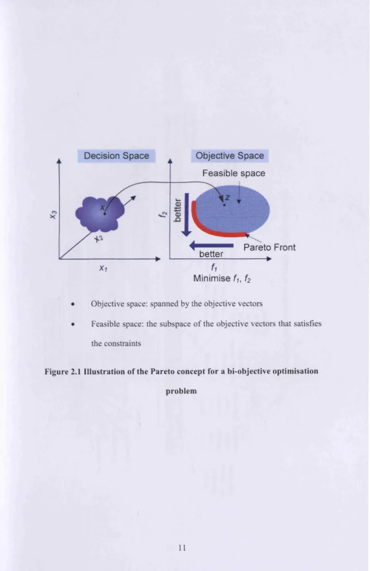
A solution a is said to be Pareto optimal if and only if there does not exist another solution that dominates it. The corresponding objective vector f (5) is called a Pareto dominant vector, or non-inferior or non-dominated vector. All the Pareto optimal solutions are known as the Pareto optimal set. The corresponding objective vectors are said to be on the Pareto front. Figure 2.1 depicts the Pareto concept for a bi-objective minimisation problem.

2.2 Multi-Objective solvers

Solving M O problem s has evolved over tim e. Initial classical approaches essentially consisted o f converting the M O problem into a SO problem w hich can be solved using traditional scalar optim isation techniques. Population-based intelligent methods have more recently been used, which allows direct generation o f trade-off curves in a single run. Taxonomy o f MO solvers is shown in Figure 2.2.

2.2.1 Classical methods

Classical approaches have been used to convert an MO problem into an SO problem by either aggregating the objective functions or optimising the most important objective and treating the others as constraints which are geared towards finding a singe solution. In order to generate a trade-off curve, the solution procedure has to be reapplied after modifying the aggregation modalities or design criteria. Although there are many classical methods, the weighted sum method is the simplest approach and probably the most widely used. Therefore only the weighted sum method is reviewed here.

Decision Space

Objective Space

Feasible space

better

Pareto Front

Minimise

• Objective space: spanned by the objective vectors

• Feasible space: the subspace of the objective vectors that satisfies the constraints

Figure 2.1 Illustration of the Pareto concept for a bi-objective optimisation problem

W e ig h te d su m x £ -C o n stra in t W e ig h te d m etr ic C la s s ic a l m e th o d s M u lti-O b je c tiv e s o lv e r s I n te llig e n t te c h n iq u e s In tera ctiv e G o a l p r o g r a m m in g M e ta -h e u r is tic a lg o rith m V a lu e fu n c tio n B e n s o n s S in g le -p o in t sto c h a s tic se a rch a lg o r ith m s S im u la te d G e n e tic a n n e a lin g A lg o r ith m P o p u la tio n -b a se d a lg o r ith m s A r tific ia l I m m u n e S y s te m s N o n -P a r e to -b a s e d a p p roach H L G A ( H a le j a & L in ’s G e n e tic A lg o r ith m ) V E G A ( V e c to r E v a lu a ted G e n e tic A lg o r ith m ) M O G A (M u lti-O b je c tiv e G e n e tic A lg o r ith m ) P a reto -b a se d ap p roach E v o lu tio n a r y A lg o r ith m s N S G A ( N o n ­ d o m in a te d (S o r tin g G e n e tic A lg o r ith m ) S P E A 2 S P E A (S tr e n g th P areto E v o lu tio n a r y S tr a te g ie s A n t C o lo n y O p tim isa tio n

N S G A - ll E v o lu tio n a r y A lg o r ith m ) N P G A (N ic h e d P areto G e n e tic A lg o r ith m ) P A E S (P a r e to A r c h iv e E v o lu tio n S tr a te g y ) S w a r m -b a s e d a lg o r ith m s P a r tic le S w arm O p tim isa tio n

I

B a c te r ia F o r a g in g O p tim isa tio n

A lg o r ith m M O P S O (M u lti-O b je c tiv e P a r tic le S w arm O p tim is a tio n )

i

2.2.1.1 W eighted sum m ethod

The weighted sum method scalarizes a set o f objectives into a single objective by pre-multiplying each objective with a user-supplied weight (Deb 2001). Although the idea is simple, the challenge is determining what values o f the weights to use. It depends on the importance o f each objective in the context of the problem and also a scaling factor. The utility function o f this method is a linear combination o f the objectives:

Minimise Wj f j(*) with > 0 and ^ = 1, Eq. 2.4

7=1 7=1

where the weights ( w; ) are chosen to reflect the relative importance the Decision Maker (DM) attaches to each o f the N objectives.

In order to generate a trade-off curve with the weighted sum method, (Kim and de Week 2005) developed the Adaptive Weighted-Sum (AWS) method. This focuses on unexplored regions by changing the weights adaptively rather than by using prior weight selections and by specifying additional inequality constraints. It produced well-distributed solutions, found Pareto optimal solutions in non- convex regions and neglected non-Pareto optimal solutions.

2.2.2 Intelligent methods

Due to the complexity o f real-world optimisation problems such as ill-defined functions and non-differentiability, it is virtually impossible to find exact algorithms. For these types of problems, meta-heuristics are a practical way to generate acceptable solutions, even though they cannot guarantee optimality. Several variants o f meta-heuristic algorithms exist including single-point stochastic search algorithms (e.g., simulated annealing (Kirkpatrick et al. 1983; Pham and Karaboga 1999)) and population-based algorithms. However, only population-based algorithms are reviewed here.

2.2.2.1 Population-based Multi-Objective solvers

This section presents some popular population-based MO algorithms. Recent studies on Evolutionary Algorithms have shown that population-based algorithms are potential candidates to solve MOOPs. They can be efficiently used to eliminate most of the difficulties with classical single objective methods such as sensitivity to the shape o f the Pareto front and the necessity o f multiple runs to find multiple Pareto solutions. Although the majority are based on Evolutionary Algorithms (EAs), the most recent are inspired from swarm intelligence such as Ant Colony Optimisation (ACO) (Dorigo et al. 1996), Particle Swarm Optimisation (PSO) (Eberhart and Kennedy 1995; Kennedy and Eberhart 1995), Artificial Immune Systems (AIS) (Forrest et al. 1994), Bacteria

Foraging Optimisation Algorithm (BFOA) (Passino 2002) and the Bees Algorithm (Pham et al. 2005).

The general structure of population-based MO solvers is similar to those used for SO solvers. However, three different steps are adopted to solve MOOPs.

1) fitness assignment controls convergence, o f which there are three methods: aggregation-based, criterion-based and Pareto-based. O f these the Pareto-based fitness assignment is the most popular and efficient technique. Figure 2.3 shows how to generate a Pareto front using population-based techniques.

2) diversity mechanisms such as niching are included to determine an individual’s fitness in order to prevent premature convergence to a region of the front.

3) a form o f elitism is applied to prevent the problem deteriorating to the point where dominant solutions may disappear from one generation to the next.

c Initialisation Decision vectors Evaluation Objective vectors Stopping criterion?

Pareto dominance sorting _Archive

Non-dominated vectors

Fitness assignment

Selection & Variation

Figure 2.3 Pareto front generation using population-based techniques

2.2.2.1.1 Genetic Algorithms (GAs)

The concept o f GA’s developed by (Goldberg 1989; Holland 1992) in the 1970s was inspired by the Darwin’s evolutionist theory explaining the origin of species. In nature, while weak and unhealthy species are faced with extinction by natural selection, the strong or healthier have a greater opportunity to pass their genes on to future generations via reproduction. In the long run, species carrying the correct combination in their genes become dominant in their population. Sometimes, during the slow evolutionary process, random changes may occur in genes. If these changes provide additional advantages in the challenge for survival, new species evolve from the old ones, but unsuccessful changes are eliminated by natural selection. In GA terminology, a solution vector is called a chromosome which consists o f discrete units called genes and a collection of chromosomes which is called a population. In the original implementation o f GA by Holland, genes are assumed to be binary digits. However, in later implementations, more varied gene types have been introduced. Normally, a chromosome corresponds to a unique solution in the solution space and it requires a mapping mechanism called an encoding mechanism between the solution space and the chromosomes. Figure 2.4 illustrates a simplified flowchart o f GA in which the population is normally randomly initialised. As the search evolves, the population eventually converges, which means that it is dominated by a single solution. GA uses two operators to generate new solutions from existing ones:

1) Crossover is the most important operator in GA. Generally, two chromosomes, called parents, are combined together to form a new chromosome called offspring. The parents are selected from existing chromosomes in the population with a preference towards fitness so that their offspring are expected to inherit good genes. By iteratively applying the crossover operator, genes o f good chromosomes are expected to appear more frequently in the population, eventually leading to convergence to an overall good solution.

2) M utation introduces random changes into the characteristics o f chromosomes, which are generally applied at the gene level. In typical GA implementations, the mutation rate (the probability o f changing the properties o f a gene) is very small, and depends on the length o f the chromosome. Therefore the new chromosome produced by mutation will not be very different from the original one. However, it plays a critical role in GA because it reintroduces genetic diversity back into the population and assists the search to escape from local optima.

Reproduction involves the selection o f chromosome for the next generation. There are different selection procedures in GA depending on how the fitness values are used. Proportional, ranking and tournament selection are the three most popular selection procedures.

Yes No ermination criterion? Mating Selection Initial population Evaluation Crossover Mutation

GA for Multi-Objective Optimisation Problems

GA is well suited to solve MOOPs as a population-based approach. The crossover operator in GA may exploit the structure o f good solutions with respect to different objectives to create new non-dominated solutions in unexpected parts o f the Pareto front. A GA does not require the user to prioritise, scale or weigh objectives, therefore it has become the most popular heuristic approach to Multi-Objective design and optimisation problems. (Jones et al. 2002) reported that 90% o f the approaches to Multi-Objective optimisation aimed to approximate the true Pareto front for the underlying problem. A majority of these used a meta-heuristic technique and 70% o f all meta-heuristics approaches were based on evolutionary approaches. (Deb 2001) and (Coello et al. 2007) are well documented regarding various versions o f Multi-Objective GAs and their applications. In addition, (Guliashki et al. 2009; Konak et al. 2006; Lee and El-Sharkawi 2008) aptly summarised them. Figure 2.5 shows a GA for MOOPs according to their work.

Vector-Evaluated Genetic Algorithm (VEGA)

Multi-Objective Genetic Algorithm (MOGA)

GA for MOOPs

Non-elitist Niched-Pareto Genetic Algorithm (NPGA)

Non-dominated Sorting Genetic Algorithm (NSGA)

— Elitist

Non-dominated Sorting Genetic Algorithm (NSGA-II) Strength Pareto Evolutionary Algorithm (SPEA)

Strength Pareto Evolutionary Algorithm 2 (SPEA 2) Pareto Archived Evolution Strategy (PAES) algorithm Pareto Enveloped based Selection Algorithm (PESA)

• Non-elitist Multi-Objective Evolutionary Algorithms

o Vector-Evaluated Genetic Algorithm (VEGA): (Schaffer 1984) suggested VEGA as the first implementation o f a real Multi-Objective Evolutionary Algorithm in 1984. He separated the selection method for each individual objective to fill up a portion o f the mating pool, which meant that each subpopulation is evaluated with respect to a different objective. Then, the entire population is thoroughly shuffled to apply crossover and mutation operators.

o Multi-Objective Genetic Algorithm (MOGA): (Fonseca and Fleming 1993) proposed MOGA in 1993, which is the simple extension o f a single objective GA. The main concept is that all non-dominated individuals are assigned the same highest possible fitness value, while dominated ones are penalised according to the population density o f the corresponding region.

o Niched-Pareto Genetic Algorithm (NPGA): (Horn et al. 1994) propounded NPGA which uses a tournament selection scheme based on Pareto dominance. The basic idea o f NPGA is: two individuals are randomly chosen and compared against a comparison subset (typically around 10% o f the population) from the entire population. When one candidate is dominated by the set and the other is not, the latter is selected. If neither or both candidates are dominated, fitness sharing is used to decide selection.

o Non-dominated Sorting Genetic Algorithm (NSGA): (Srinivas and Deb 1994) postulated NSGA based on several layers o f classifications of the individuals. Before selection is performed, the population is ranked on the basis of non-domination. However, it is not very efficient because Pareto ranking has to be repeated over and over again.

• Elitist Multi-Objective Evolutionary Algorithms: The elitist Evolutionary Multi-Objective Optimisation (EMOO) methodologies include an elite- preservation mechanism in their procedures. The non-elitist EMOO algorithms do not use such a mechanism and usually perform worse than the elitist algorithms. In the context o f Multi-Objective optimisation, elitism usually, (although not necessarily), refers to the use o f an external population (also called secondary population) to retain the non-dominated individuals found along the evolutionary process. Following the theory offered by (Zitzler and Thiele 1999), most researchers began to incorporate external populations in their EMOO algorithms and the use o f this mechanism became common practice.

o Non-dominated Sorting Genetic Algorithm-II (NSGA-II): (Deb et al. 2002) introduced NSGA- II as an improved version of NSGA. It adopts a Crowding Distance mechanism for diversity. Its elitist mechanism combines the best parents with the best offspring obtained, instead o f using an external memory.

o Strength Pareto Evolutionary Algorithm (SPEA): (Zitzler and Thiele 1999) introduced SPEA which uses an archive containing non-dominated solutions previously found (the so-called external non-dominated set). At each generation, non-dominated individuals are copied to the external non-dominated set. For each individual in this external set, a strength value is computed. The fitness o f each member of the current population is computed according to the strengths o f all external non-dominated solutions that dominate it. Although this approach does not require a niche radius, its effectiveness relies on the size o f the external non- dominated set. If its size grows too large, it slows down the search procedure.

o Strength Pareto Evolutionary Algorithm 2 (SPEA 2): This was also developed by (Zitzler and Thiele 1999) to address some o f the major drawbacks o f SPEA. It has three main differences with SPEA:

1) It incorporates a fine-grained fitness assignment strategy which takes into account for each individual the number o f individuals that dominate it and the number o f individuals by which it is dominated. 2) It uses a nearest neighbour density estimation technique which guides

the search more efficiently.

3) It has an enhanced archive truncation method that guarantees the preservation of boundary solutions.

o Pareto Archived Evolution Strategy (PAES) algorithm: (Knowles and Come 2000) introduced PAES consists o f a 1+1 evolution strategy (i.e., a single parent that generates a single offspring) in combination with a historical archive that records the non-dominated solutions previously found. The role of the external archive is limited to storing the non- dominated solutions and provides a source of comparison for ranking candidate solutions. However, archive members are not involved in the mutation and crossover procedures. The interesting feature o f this algorithm is in the adaptive grid at the heart o f its diversity and niching mechanisms. The objective space is divided in a recursive manner, thus creating a multi-dimensional co-ordinate system, or grid, over the objective space. A crowding-based fitness sharing mechanism is applied by determining the location o f solutions within this grid and estimating the density o f solutions per cell. Individuals corresponding to solutions in the less crowded cells have higher fitness,

o Pareto Envelope based Selection Algorithm (PESA): (Come et al. 2000) suggested PESA which combines the good aspects o f SPEA and PAES. Like SPEA, PESA carries two populations (a smaller EA population and a larger archive population). Non-domination and the PAES crowding concept are used to update the archive with the newly created child solutions.

2.2.2.1.2 Ant algorithm

The Ant System (AS) developed by (Dorigo 1992) was the original ant algorithm. Since then several improvements to the Ant System have been devised. It was inspired by colonies o f real ants that deposit a chemical substance on the ground called pheromone. This substance influences the behaviour of the ants as they tend to take those paths where there is a larger amount of pheromone. Pheromone trails can thus be seen as an indirect communication mechanism among ants. Three main ideas from actual ant colonies that have been adopted are:

• Indirect communication through pheromone trails

• Shortest paths tend to have a greater pheromone growth rate

• Ants have a higher preference (with a certain probability) for paths that have a larger quantity o f pheromone

Ant Colony Optimisation (ACO) was introduced by (Dorigo et al. 1996) as a novel nature-inspired metaheuristic for solving combinatorial optimisation problems such as the Travelling Salesman Problem (TSP) which entails the cost function to be minimised. The simple ACO can be stated as given by (Bonabeau et al. 1999; Camazine et al. 2003; Dorigo and Stutzle 2004; Engelbrecht 2006): A combinatorial optimisation problem entails the cost function to be minimised. A candidate solution is defined as a sequence o f parameters visualised as a path through several nodes. Each node corresponds to one o f the solution’s

parameters. Moving from one node (z) to another (/) is carried out by the probability (Eq. 2.5).

where

transition probability

Ty : posterior effectiveness o f the move from node z to node j , as expressed in the pheromone intensity o f the corresponding link (z',y)

rjy: prior effectiveness o f the move from z to j (i.e., the attractiveness or desirability of the move) and it is computed using some heuristic

a : parameter to control the influence o f Ty

f t: parameter to control the influence of rjtJ

N- : set o f feasible nodes for ant k when located on node z

The pheromone concentrations, Ty, indicate how profitable it has been in the past to make a move from z to j\ serving as a memory o f previous best moves. Pheromone evaporation is implemented as given in Eq. 2.6. After completion of a path by each ant, the pheromone on each link is updated according to Eq. 2.7.

Eq. 2.5

0

Tij (0 <- (! - P^ij (t) with p g [0,1] Eq. 2.6

The constant, p , specifies the rate at which pheromone evaporates, causing ants to ‘forget’ previous decisions controlling the influence o f search history. For example, if p is a large value, pheromone will evaporate rapidly and vice versa. The greater the evaporation, the more random the search becomes which means that it is facilitating a better exploration. When p = 1, the search is completely random. r„ (' + l)= r,,(0 + A r„ (r) Eq. 2.7 A rf (/) = 2 > r ‘ (r) E q .2 .8 k = \ where nk : number o f ants

At* (/): amount o f pheromone deposited by ant k on link (i,j) at time step t.

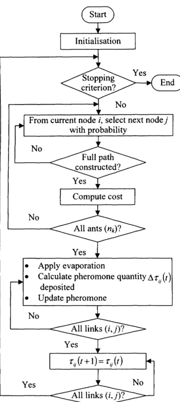
Figure 2.6 illustrates the flowchart o f ACO for solving combinatorial problems.

ACO for M ulti-Objective O ptim isation Problem s

The first implementations o f ACO algorithms utilised only one colony o f ants to construct solutions. However, multiple colony algorithms have been adapted to use multiple colonies, with the main objectives of mitigating stagnation and

minimising the chances of being trapped in local minima. Multiple colonies have also been used to solve MOOPs and it was one o f the first applications o f multiple colony ACO. MOOPs are solved by assigning to each colony the responsibility o f optimising one o f the objectives. If nc objectives need to be optimised, a total o f nc colonies are used. Colonies cooperate to find a solution that optimises all objectives by sharing information about the solutions found by each colony. (Tippachon and Rerkpreedapong 2009) adopted this Multiple Ant Colony System (MACS) for the optimal placement o f switches and protective devices in electrical power distribution systems. (Colson et al. 2009) also employed this algorithm for solving a Micro-Grid (MG) Multi-Objective power management problem.

Another version o f ACO for solving MOOPs is Population-based ACO (PACO) which was introduced by (Guntsch and Middendorf 2002). (Angus 2007) applied this algorithm to Multi-Objective function optimisation. The defining difference between PACO and canonical ACO algorithms is the method used for storing solutions. Most traditional ACO algorithms store solution information from an (artificial) ant in a pheromone matrix only, PACO stores solutions in a population and then uses this population to make adjustments to the pheromone matrix. However, PACO still uses the core principles o f ACO which include stepwise construction (solutions are constructed one piece at a time) and the use o f global information in constructing solutions.

Yes No No No All ants («*)? Yes No All links (/,/)? Yes No Yes All links (1,7)? Stopping criterion? Full path ^constructed? Compute cost Initialisation

From current node i, select next node j with probability

Apply evaporation

Calculate pheromone quantity At (?) deposited

Update pheromone

Figure 2.6 Flowchart of Ant Colony Optimisation algorithm

2.2.2.1.3 Particle Swarm Optimisation (PSO)

Kennedy and Eberhart proposed a population-based stochastic optimisation called ‘Particle Swarm Optimisation (PSO)’ in 1995 (Eberhart and Kennedy 1995; Kennedy and Eberhart 1995) inspired by the collective behaviour of social animals such as bird flocking or fish schooling (Engelbrecht 2006; Kennedy et al. 2001; Van den Bergh 2006). A PSO algorithm maintains a swarm of particles and an individual particle, which represents a potential solution, moving through a multi-dimensional search space to approach the optima. Figure 2.7 illustrates the flowchart for PSO. Initially, the number o f particles are randomly created and set into motion through the search space (‘Initial population’ in Figure 2.7). A particle has its own position and flight velocity, which is constantly adjusted during the optimisation process. For a better position (fitness), each particle adjusts its position based on its own experiences (personal best: ‘pbest’) as well as that of the entire swarm (global best: ‘gbest’) at each generation. Eq. 2.9 represents the formula to change the position o f the particle by adding a velocity, ^ ( / + l), to the current position ( X ^ t ) ) . The velocity formula is shown in Eq.

2.10.

*,.(' + !)= * , ( 0 + ^ + 1) Eq.2.9

where

i ( i = 1,2, . . . , ri): index o f individual particles in the swarm n: total number of particles in the swarm

t: discrete time steps

X t{t + l) : updated position of particle i at next step (/+1) which is calculated using the current position with updated velocity

X t (/): current position o f particle i in the search space at step t Vi( t +1): updated velocity o f particle i at next step (/+1)

v,j

(tipbesfj^ -x^ {t)\+c2r2]

j O' - 1 , 2 , . .m): index o f dimensional search space m: number o f dimensional search space

vjy(/ + l): velocity o f particle i in dimension j at step (/+1) calculated by using the current velocity and the distance from pbesU to gbestt w: inertia weight that controls the impact o f previous velocity

vtj (/): velocity o f particle i in dimension j at step / which is confined to the range [vmn, ] to control excessive roaming o f particles outside the search space

xjy(/): position o f particle i in dimension j at step /

ci and eg positive acceleration constants used to scale the contribution o f the cognitive and social components respectively

r{j(t) andr2j{t)\ random values in the range [0,l] sampled from a uniform distribution

pbesty (/): personal best position o f particle i at step t since the first step gbestj(t) : global best position at step /, which is the best position

discovered by any o f the particles to date

Y es N o Y es N o Termination criterion?

Outside the pre-defined

'^ ■ ^ h y p e r c u b e ? ^ ^

Reintegrate it to its boundaries Update the velocity and

_______ position_______ Initial population

Update ‘pbest’ and ‘gbest’ Evaluation

Under the guidance o f these two updating rules (Eq. 2.9 and 2.10), the particles will proceed toward the best position found so far. This driving force makes the PSO algorithm search to find the optimal solutions.

PSO for Multi-Objective Optimisation Problems

The basic PSO cannot be applied directly to solve MOOPs (Engelbrecht 2006). This is due to the velocity update equation where the social component causes all particles to converge on one point. Changing conventional single objective PSO to a Multi-Objective PSO (MOPSO) requires redefining the global best because there is no absolute global best in the Multi-Objective PSO procedure, but rather a set of non-dominated solutions. Therefore choosing the global best to guide the swarm becomes a nontrivial task in the Multi-Objective domain (Abido 2009). Many researchers have proposed several PSO-based MO solvers which are generally categorised by three methods:

• Aggregation-based methods: One o f the simplest approaches to deal with MOOPs, is to define an aggregate objective function as a weighted sum of the objectives, because uni-objective optimisation algorithms can be applied without any changes to the algorithm to find optimum solutions. (Parsopoulos and Vrahatis 2002a, b) applied this aggregation method to a number o f standard benchmarking functions, but there are numerous problems. For example, the

algorithm has to be applied repeatedly to find different solutions. Even for repeated applications, there is no guarantee that different solu