Article
An Eigenvector Centrality for Multiplex Networks
with Data
Francisco Pedroche1 , Leandro Tortosa2 and José F. Vicent2,*
1 Institut de Matemàtica Multidisciplinària, Universitat Politècnica de València, E-46022 València, Spain;
2 Department of Computer Science and Artificial Intelligence, University of Alicante, Campus de San Vicente,
Ap. Correos 99, E-03080 Alicante, Spain; [email protected] * Correspondence: [email protected]; Tel.: +34-965-903900
Received: 10 May 2019; Accepted: 3 June 2019; Published: 5 June 2019 Abstract: Networks are useful to describe the structure of many complex systems. Often, understanding these systems implies the analysis of multiple interconnected networks simultaneously, since the system may be modelled by more than one type of interaction. Multiplex networks are structures capable of describing networks in which the same nodes have different links. Characterizing the centrality of nodes in multiplex networks is a fundamental task in network theory. In this paper, we design and discuss a centrality measure for multiplex networks with data, extending the concept of eigenvector centrality. The essential feature that distinguishes this measure is that it calculates the centrality in multiplex networks where the layers show different relationships between nodes and where each layer has a dataset associated with the nodes. The proposed model is based on an eigenvector centrality for networks with data, which is adapted according to the idea behind the two-layer approach PageRank. The core of the centrality proposed is the construction of an irreducible, non-negative and primitive matrix, whose dominant eigenpair provides a node classification. Several examples show the characteristics and possibilities of the new centrality illustrating some applications.
Keywords: eigenvector centrality; networks centrality; two-layer approach PageRank; multiplex networks; biplex networks
1. Introduction 1.1. Literature Review
The identification of the most relevant nodes in complex networks has caught the attention of researchers because of its theoretical significance [1]. The idea of importance of a vertex in complex networks is associated with the concept of centrality and it is a basic question in analysing complex networks.
Recently, it has been accepted that some complex systems can be integrated by multilayer networks that characterize different interactions [2–4]. Originally, the termmultiplex networkwas applied to social networks and it indicated that the same person has more than one relationship [5]. Nowadays, it is a type of multilayer network in which a set of links determines a different layer [6,7].
We understand multiplex networks as a non-linear superposition of complex networks, where some components interact through a variety of different relationships which are conceptualized as different layers (see [8] for a formal introduction to the subject of multiplex networks).
Multiplex networks have been applied in wide areas of science, such as transportation networks [9], social networks [10], financial networks [11] or biological networks [12]. For instance, in a
transportation network, each layer may represent a different mode of transportation or, in collaboration networks, the different layers may represent several topics of the collaboration. In this regard, it is interesting to have the centrality of these multilayer structures [13,14].
In [15], the authors calculate the centrality of multiplex networks based on Multiplex PageRank. There are other centrality measures that associate a different influence to the links of the layers with the aim of pondering their contribution to the node centrality [13,14]. Likewise, Ribalta et al. [16] re-define an intermediation centrality to take into account the structure of multiplex networks, proposing an algorithm to compute it efficiently.
An extension of the eigenvector centrality to multiple networks is presented in [13] , highlighting the relationships between the different centrality measures. Their starting question is: How can one consider all the interactions between the sub-networks assuming that not all of them have the same importance? Spatocco et al. [17] propose a new framework called TaCMM that can encode specific dependencies between the subnets of multiplex networks to define semantic-aware centrality measures.
An approach to the classic PageRank based on a two-layer network is presented in [18]. The authors’ proposals draw from the idea that the importance of the nodes is given by two factors: the topology of the network and the teleportation from one node to another. Following this approach, Agryzkov et al. [19] design and implement an adaptation of the PageRank algorithm for spatial networks with data to the two-layer approach PageRank.
1.2. Main Contribution
In the present paper, the main focus is to provide a measure of centrality for multiplex networks based on the idea behind the eigenvector centrality. The proposed model adapts the eigenvector centrality for single-layer networks with data [20] and implements the two-layer approach PageRank concept [18]. The principal feature that distinguishes this measure is that it calculates the centrality in multiplex networks where the layers have different relationships between nodes and where each layer has a dataset associated with their nodes. The key of this model is the ease with which we can measure the impact of the data presented in a network when calculating the nodes’ centrality. The versatility of the proposed measure allows to work with data from different sources or types (real, virtual, ...) and evaluate its importance within the network.
It is certainly useful to use this centrality in different types of networks. For instance, in social networks, it is possible to consider different relationships between nodes such as vicinity, member-ship, coworker-ship, etc. Epidemic spreading in multilayer networks is probably one of the most immediate applications of multilayer networks. In [21], the new approach allows studying scenarios in which two or more diseases interact cooperatively or competitively. However, there are other potential applications such as the improvement in the recommender systems [22,23] or networks of Public Safety [24,25].
The paper is structured as follows. Section2is devoted to describe well-established centrality models for single-layer networks which constitute the basis for the proposed centrality of multiplex network. In Section3, it is possible to show how the proposed measure gives distinct results in networks with different datasets. A biplex network about jazz musicians born in the firs decades of the 20th century is constructed and analyzed, obtaining the most relevant nodes. The discussion of the results are given in Section4. Finally, in Section5some conclusion are presented.
2. Methodology
In this section, the well-established models that constitute the core of the proposed centrality are described in detail. Later, an algorithm summarizing the required calculations to obtain the measure for multiplex networks is presented and analysed.
LetG= (N,E)be a connected graph with the adjacency matrixA= aij , with aij = ( 1 if(i,j)is a link, 0 otherwise.
2.1. The Eigenvector Centrality for Networks with Data
In [26], Bonacich presented the classical eigenvector centrality which measure the importance of a node depending on its connections. However, we can consider the possibility that not all the links are equally relevant. Taking this into account, we argue that the centrality does not only depend on the quantity of its links, but also on the degree of its adjacent nodes.
Denoting byxithe centrality of the nodei, it is possible to measure the importance of each node
with the expression,
xi= 1 λ n
∑
j=1 aijxj, (1)whereaijare the elements of the adjacency matrix corresponding to the rowi, andλis a constant. Defining the centrality vector asx= (x1,x2, . . .), the expression (1) can be rewritten as
A·x=λx. (2)
From the expression (2), x is an eigenvector of the adjacency matrix A associated with the eigenvalue λ. Taking into account that A is non-negative and irreducible and using the Perron–Frobenius theorem, there exists and eigenvector associated with the maximum eigenvector (in absolute value) with positive entries. This vector is the eigenvector centrality.
This classical eigenvector centrality only takes into account the topology and the links of the neighbouring nodes. It does not incorporate any other data of the spatial network.
In [20], Agryzkov et al. present a new centrality measure for networks that takes into account geo-located data associated with the network. Besides, this measure allows to weight the contribution of the topology in the final classification.
The main idea of the model is the construction of adata vectorvwith all the information present in the network. This vector is normalizedv∗and allows to establish theimportanceof an edge between nodesiandjas
wij =v∗(i) +v∗(j).
Repeating the computation for all edges, a weight matrixWfor the data is constructed. With the aim to avoid null elements in the weight matrixW, abasic minimum level of importanceis introduced, denoted byα. A matrixA∗is constructed summarizing the importance of the topology of the network and the data present in it.
Algorithm 1(Eigenvector centrality for network with data).LetG= (N,E)be a primary graph withnnodes,
Athe adjacency matrix,Dthe data vector andv0the balanced vector for data. Let us denote by◦the Hadamard
matrix product.
1 The data vectorv=D·v0is constructed.
2 Normalization ofv.
v∗= 1
maxivi v.
3 The weight matrixW
wij=v∗(i) +v∗(j) is constructed.
4 Calculateαusing the expressionα=min vi∗/10, v∗i 6=0.
5 Takee, according to the expressione< 101α.
6 FromA,W, andα,econstructA∗as
A∗=A◦(W+αJ) +eJ. 7 Compute the dominant eigenpair ofA∗,(λ1,x1).
8 FromAandx1compute the eigenvector centrality for networks with data CVP as
CVP= 1
λ1
[Ax1+x1].
WhereJis a matrix with 1’s in all its entries. It is relevant to remark, as a special characteristic of this model, that the data associated with the network allow to quantify and qualify the information located in their environments.
Based on the Agryzkov et al. [20] model some small modifications are introduced in order to design and implement the centrality measure for multiplex networks.
First, the definition of the parameterαhas been modified slightly, reducing the value of thebasic
minimum level of importanceof data in the global network. Now,αis calculated as α=min(v∗i)/10, v∗i 6=0.
Specifically, the weight matrixWis now defined as
wij=v∗(i) +v∗(j) +α.
The introduction of thebasic minimum level of importanceassociated with the edges in matrix
Wis because of the own centrality, where the importance of a node is given by the influence of its neighbours. It can be said that a node with no data is always influenced by the global dataset of the whole network, even if the nodes are not directly connected to it.
Consequently, the definition of the matrixA∗is now
A∗= A◦W+eJ.
In the step 8 of Algorithm 1, the centrality of the nodes is calculated from A and x1 by the expression
CVP= 1
λ1[Ax1+x1], (3)
which is different from the classic eigenvector centrality model computed using the expression (1). In (1), the centrality of a node is only determined by the influence of the nodes to which it is connected. However, in the eigenvector centrality with data, the termx1is added in the expression (3), which
represents the importance of the node itself due to the data associated with it. This is a small variant that is introduced with respect to the classic eigenvector centrality, which aims to evaluate the importance of data associated with a particular node.
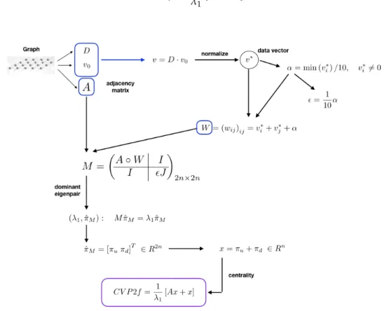
Figure1shows a schematic representation of the eigenvector centrality model proposed in [20] for networks with data taking into account the modifications proposed.
Figure 1.Eigenvector centrality modified for networks with data.
2.2. The Two-Layer Approach Pagerank
A two-layer approach PageRank was propose by Pedroche et al. in [18]. The key is to consider the PageRank model as a process divided into two parts: one related to the topology of the network and the other related to the probability of jumping between two nodes in the network, following a criterion that there is the same probability among all of them.
In [18], the authors realize that the classification obtained by the PageRank graph G can be understood as the stationary distribution of a Markov chain that occurs in a two-layer network
l1, a physical layer:the networkG.
l2, a teleportation layer:the network given by the personalized vector.
Within this framework, a block matrixMAis constructed, where each diagonal block is associated
with every layer. Hence,MAcan be constructed as
MA=
αPA (1−α)I
αI (1−α)evT
!
∈R2n×2n. (4)
whereMAdefines a two-layer Markov chain.
Remark that matrixPAis a probability matrix defined as
PA=pij =
( 1
cj ifaij6=0,
0 otherwise, 1≤i,j≤n, wherecjis the sum of thej-th column of the adjacency matrixA.
SinceMAis irreducible and primitive, Pedroche et al. [18] defined thetwo-layer approach PageRank
of an adjacency matrixAas the vector ˆ
πA=πu+πd ∈Rn,
where there is a unique normalized and positive eigenvector of matrixMAgiven byπTu πdTT∈R2n.
The idea of separating the centrality based on the PageRank concept into two layers, differentiating the topological part of the network from the concept of personalization vector, can be extrapolated to multilayer networks, as the authors demonstrate in [18].
2.3. Adapting the Two-Layer Pagerank Approach for Eigenvector Centrality
In this section, a modification of the eigenvector centrality described in Section2.1is presented. It is based into the two-layer approach PageRank technique described in Section2.2. A 2×2 block matrix is used to distinguish the topology and the teleportation layer. But some previous reasoning are required to understand the similarity of both models.
The idea of the combination of a physical layer and a teleportation layer in PageRank measure, differentiating the topological part of the network from the idea of jumping in a random way from one node to other, can be applied in this case in a similar way. Thus, let us consider a first layer related to the quantity of data from the topology of the network and a second layer where a residual importance of the data is considered globally in the network, regardless of where they are located. The first layer may be calledtopological datawhile the second one may be calledresidual data.
The key of this model lies in the construction of the matrixMgiven by
M= A◦W I
I eJ
!
∈R2n×2n. (5)
The first diagonal block ofMis related to thetopological datalayer and may be expressed by the Hadamard productA◦W, whereAis the adjacency matrix andWis the weight matrix constructed from the quantity and location of data in the network. This block clearly reflects the influence of data regarding the topology of the network. The second diagonal block is related to theresidual datalayer and is expressed by the producteJthat summarizes the influence of a residual data value at a global network scale. In this second block, we introduce thebasic minimum level of importancein the definition of the weight matrixW. This is in accordance with the idea of teleportation, considering equally likely the jump from one node to another, in a random way.
In Figure2, a schematic representation of the eigenvector centrality model [20] is presented taking into account the two-layer approach PageRank.
Note thatMis irreducible since any node has a path to any other node, and this is independent of whetherAis irreducible or not. Besides,Mis also non-negative and primitive (since it is known that an irreducible nonnegative matrix with a nonzero diagonal element is primitive [27]). Therefore, the eigenvector centrality corresponding toMis well defined in the sense that the dominant eigenvalue is unique and we can find an associated eigenvector with all its entries positive.
Consequently, because of the good spectral characteristics ofM, the eigenpar(λ1, ˆπM)is obtained,
whereλ1is the dominant eigenvalue and
h
πuTπdT
iT
∈R2n,
is the unique positive eigenvector of matrixMgiven by (5). Therefore,
x=πu+πd ∈Rn,
This centrality, that adapts the two-layer approach for PageRank to the eigenvector centrality for networks with data, is denoted as CVP2f and may be calculated by the expression
CVP2f = 1 λ1
[Ax+x]. (6)
Figure 2.Eigenvector centrality following the two-layer approach PageRank.
2.4. The Eigenvector Centrality for Multiplex Networks with Data
Taking as a reference the model described in Figure2, it is possible to extend the centrality measure to the case of multiplex networks, where all the layers have the same nodes and the differences are in the relationships among them.
Let us consider a multiplex network M = (N,E,S) with layers S = (l1,l2, . . . ,lk). Then,
an eigenvector centrality is defined by associating to each layerli a two-layer approach as it was
described in Section2.2. Moreover, the transition between these layers must be allowed.
To begin with, a biplex networks M = (N,E,S) with two-layerS = (l1,l2)and adjacency matrices A1,A2 ∈ Rn×n are considered. We write the following elements for every layerli, (for i=1, 2):Didata matrix,v0ibalanced vector,Wiweight matrix, andαi,eiparameters associated with
the data vector.
It is possible to construct the 4n×4nmatrixMBIas
MBI= 1 2 A1◦W1 I I 0 I A2◦W2 0 I I 0 eJ1 eJ2 0 I eJ1 eJ2 . (7)
The spectral characteristics ofMare inherited by the fact thatMBIis built non-negative, irreducible
and primitive. Therefore, there exists a unique dominant eigenvalue and an eigenvector associated with it with all its elements positive. That is, the eigenvector
ˆ
πBI = (πu1,πu2,πd1,πd2) ∈R
is associated with the dominant eigenvalueλ1. This vector is the basis to obtain the classification vector. Therefore, a unique vector is obtained
x= 1
2(πu1+πu2+πd1+πd2) ∈R
n, (9)
with all its elements positive.
Regarding to the calculation of the centrality, we do not have a single adjacency matrix as in the case of monoplex networks, since there is an adjacency matrix for each layer of the network. It is reasonable to think about constructing a global adjacency matrix of the network that reflects the connections between nodes in all the layers of the network. We can call this general matrix asglobal adjacency matrixand denote it byAG. This matrix is defined as
AG =AG(i,j) = (
1 if nodes i and j are linked in any layer (l1,l2),
0 otherwise. (10)
Therefore, if this centrality is denoted as CVPBI, it can be calculated by the expression
CVPBI = 1
λ1
[AGx+x],
whereAGis the global adjacency matrix given by (10).
The following algorithm summarizes the steps required to calculate the CVPBI centrality. Algorithm 2(Eigenvector centrality for biplex networks). LetM = (N,E,S), with layersS = (l1,l2)and
adjacency matrices A1,A2 be a biplex network withn nodes. LetD1,D2 be the data matrices for layers
l1,l2, respectively.
1 Construct the weighted vectorsvi=Di·v0i, fori=1, 2. 2 Normalization ofvi, fori=1, 2.
vi∗ =
1 maxj(vi)j
vi.
3 Construct the weighted matricesWi, fori=1, 2, as
Wi= wij i=vi ∗(i) +v i∗(j). 4 Computeαi, fori=1, 2, using the expressionαi=min v∗i
/10, v∗i 6=0. 5 Obtainei, according to the expressionei<101αi.
6 FromAi,Wi, andαi,eiconstructMBIas
MBI= 1 2 A1◦W1 I I 0 I A2◦W2 0 I I 0 e1J e2J 0 I e1J e2J .
7 Compute the dominant eigenpair ofMBI,(λ1,πˆBI).
8 Computexfrom the expression9.
9 ComputeAGtheglobal adjacency matrixusing expression (10). 10 FromAGandxcompute the centrality
CVPBI= 1
λ1
[AGx+x].
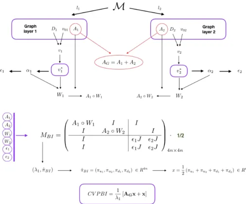
In Figure3, a scheme of the eigenvector centrality algorithm for biplex networks is presented.
Figure 3.Eigenvector centrality CVPBI for biplex networks.
This biplex measure provides a ranking vector of the nodes according to their importance. This classification is obtained from the importance of the nodes in two layers where the nodes are the same and it changes the links between the nodes and the data associated with them.
Remark that the MBI is built for biplex networks. But, it can be extended for multiplex
networks with k layers {l1,l2, . . . ,lk}, defining the adjacency and data matrices {A1,A2, . . .Ak}
and{D1,D2, . . . ,Dk}. The matrixMBIis Mmulti= 1 k M1,1 M1,2 M2,1 M2,2 ! with M1,1= A1◦W1 I · · · I I A2◦W2 · · · I · · · · I I · · · Ak◦Wk , (11) M2,2 = e1J e2J · · · ekJ e1J e2J · · · ekJ · · · · e1J e2J · · · ekJ . (12)
andM1,2,M2,1are diagonal matrices with the identityInin its blocks.
The centrality for multiple layers may be denoted as CVPM and will be given by the expression
CVPM= 1
λ1
whereAGis the global adjacency matrix given by
AG =AG(i,j) = (
1 if nodes i and j are linked in any layer (l1,l2, . . . ,lk)
0 otherwise.
andxis the eigenvector ofMmultiassociated with the dominant eigenvalueλ1. 3. Results
In this section, we present some numerical examples of the theoretical models studied in Section2 for different types of networks and sizes. These examples allow the establishment of characteristics and properties of the centralities developed, with special emphasis on the possibilities offered by an eigenvector centrality for multiplex networks.
As was discussed in Section 2.2, the way in which the final centrality is calculated in the measures described in this paper differs from the way in which it is calculated in the classical model, as can be shown looking at the expressions (1) and (3). To compare the results of centralities when applying both expressions, we distinguish between two measures of centrality, such as:
CVPThe eigenvector centrality for networks with data, using expression (3).
CVPclassicThe eigenvector centrality with data calculating the centrality using the expression (1). We will refer to this model asclassic eigenvector centrality with data.
Therefore, the different centralities involved in these examples are: CVPclassicThe classic eigenvector centrality with data.
CVPThe eigenvector centrality for networks with data.
CVP2fThe eigenvector centrality based on the two-layer approach PageRank idea. CVPBIThe eigenvector centrality for multiplex networks.
All the numerical tests have been carried out by implementing these centralities in R [28], a free software under the terms of the GNU project. It constitutes a language and environment specially efficient for computing and graphics.
Firstly, one-layer networks (monoplex) are used to compare the results obtained for the CVPclassic, CVP, and CVP2f centralities, in order to subsequently develop a discussion on the coherence of the measures defined with respect to the traditional eigenvector centrality. Later, some examples of the CVPBI centrality for particular biplex networks are described in detail.
3.1. Monoplex Networks
Let G1 = (N,E) be a simple graph with 10 nodes where N ={1, 2, . . . , 10} and
N ={(1, 2),(1, 3),(2, 4),(3, 4),(4, 5),(5, 6),(5, 7),(5, 8),(6, 7),(6, 10),(7, 8),(7, 9),(7, 10),(8, 9),(9, 10)}. Let us consider the following datasetsD1,D2andD3:
1 2 3 4 5 6 7 8 9 10 α e
D1 8 1 8 8 1 1 1 1 1 1 1/80 1/800
D2 1 1 1 10 0 0 10 0 0 0 1/100 1/1000
D3 10 2 2 2 2 2 10 2 2 2 2/100 2/1000
Now, we perform the calculations of the CVPclassic, CVP, and CVP2f eigenvector centralities, using the expression (1) and the Algorithms 1 and 2, respectively. The results are shown in Table1.
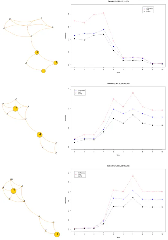
The numerical results of Table1are represented graphically in Figure4. The graphs has been drawn on the left, while the values of centralities are shown in the right column. It is observed that the size of each vertex in the graphs is proportional to the amount of data associated with it. Thus, for example, in the upper part where the data setD1is evaluated, the nodes 1, 3 and 4 are observed
with a larger size, since they have the greatest quantity of data, specifically 8. In the following section a brief analysis of the characteristics of these centralities that emerge from this example is carried out, with special emphasis on the differences between the classical model of eigenvector centrality and that proposed by Agryzkov et al. [20].
Figure 4.Eigenvector centralities CVPclassic, CVP, and CVP2f for the graphG1, using datasetsD1,
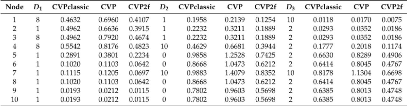
Table 1.CVPclassic, CVP, and CVP2f eigenvector centralities for the simple graphG1.
Node D1 CVPclassic CVP CVP2f D2 CVPclassic CVP CVP2f D3 CVPclassic CVP CVP2f
1 8 0.4632 0.6960 0.4107 1 0.1958 0.2139 0.1254 10 0.0118 0.0170 0.0075 2 1 0.4962 0.6636 0.3915 1 0.2232 0.3211 0.1889 2 0.0293 0.0352 0.0186 3 8 0.4962 0.7920 0.4674 1 0.2232 0.3211 0.1889 2 0.0293 0.0352 0.0186 4 8 0.5542 0.8176 0.4823 10 0.4629 0.6681 0.3944 2 0.1777 0.2018 0.1174 5 1 0.2891 0.3801 0.2234 0 0.9858 1.2528 0.7425 2 0.6630 0.8289 0.4906 6 1 0.1020 0.1103 0.0642 0 0.8668 1.0473 0.6212 2 0.6414 0.8045 0.4767 7 1 0.1115 0.1205 0.0697 10 0.9883 1.4079 0.8352 10 0.8178 1.1304 0.6698 8 1 0.1020 0.1103 0.0642 0 0.8668 1.0473 0.6212 2 0.6414 0.8045 0.4767 9 1 0.0193 0.0212 0.0115 0 0.7802 0.9603 0.5698 2 0.6385 0.8013 0.4748 10 1 0.0193 0.0212 0.0115 0 0.7802 0.9603 0.5698 2 0.6385 0.8013 0.4748
3.2. A Simple Biplex Network
In this section, we study the example of a simple biplex network constituted by 10 nodes and with two layers. In this case, the links between the nodes in the different layers have been generated randomly, while the data has been directly associated on the nodes in a simulated way to establish possible differences in the centrality values for each layer. So, let M1 = (N1,E1,S1)be a biplex network with nodes N1 = {1, 2, . . . , 10}, with layers S1 = (l1,l2)and adjacency matrices A1,A2 given by A1= 0 1 0 0 0 1 0 1 0 0 1 0 1 0 0 1 1 0 1 0 0 1 0 0 0 1 0 0 1 1 0 0 0 0 1 0 0 0 1 0 0 0 0 1 0 1 1 0 0 1 1 1 1 0 1 0 1 0 0 0 0 1 0 0 1 1 0 1 0 0 1 0 0 0 0 0 1 0 0 0 0 1 1 1 0 0 0 0 0 0 0 0 1 0 1 0 0 0 0 0 A2= 0 0 1 0 0 0 1 0 1 0 0 0 0 1 0 0 1 0 1 1 1 0 0 0 1 1 1 1 0 0 0 1 0 0 0 1 0 0 0 0 0 0 1 0 0 1 1 0 0 1 0 0 1 1 1 0 1 0 0 0 1 1 1 0 1 1 0 0 0 0 0 0 1 0 0 0 0 0 1 0 1 1 0 0 0 0 0 1 0 1 0 1 0 0 1 0 0 0 1 0 .
LetD1,D2be the data vectors for layersl1,l2, respectively,
D1= [1, 1, 1, 10, 1, 1, 1, 10, 1, 10]T, D2= [1, 1, 10, 1, 1, 1, 10, 1, 1, 1]T.
It is observed that in layer 1 the largest amount of data has been assigned to those nodes that have less connectivity, that is, degree 2. However, in layer 2 just the opposite is done, the largest amount of data has been assigned to the nodes that have greater connectivity (degree 5).
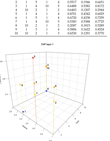
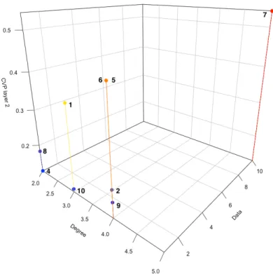
In Table2, we have reflected the following information about each node of the network: the dataD1,D2corresponding to layersl1andl2, respectively, the connectivity in each layer (dgl1, dgl2), the eigenvector centrality for layerl1(CVPl1), its eigenvector centrality for layerl2(CVPl2) and, finally, the eigenvector centrality for the biplex network CVPBI calculated from Algorithm 2. Data in Table2 may be visualized by the graphs of Figures5–7respectively.
Algorithm 2 have been run taking this network with these datasets. The results for the centrality are summarized in Table2.
Table 2. Classic eigenvector centrality for layers and CVPBI centrality for the simple biplex networkM1. Node D1 dgl1 D_2 dgl_2 CVPl1 CVPl2 CVPBI 1 1 3 1 3 0.2438 0.3548 0.6833 2 1 5 1 4 0.5517 0.1946 0.6651 3 1 4 10 5 0.6488 0.5382 0.8172 4 10 2 1 2 0.6403 0.1207 0.2944 5 1 4 1 4 0.8701 0.4342 0.6029 6 1 5 1 4 0.6720 0.4338 0.7259 7 1 4 10 5 0.5383 0.5388 0.7725 8 10 2 1 2 0.2087 0.1815 0.5289 9 1 3 1 4 0.5806 0.1622 0.4524 10 10 2 1 3 0.6530 0.1291 0.3770
Figure 6.Eigenvector centrality CVPl2.
Figure 7.Eigenvector centrality CVPBI.
3.3. A Jazz Musicians Biplex Network
An example of a biplex network related to the history of jazz is shown in this section. Among the many jazz artists that emerged between 1900 and 1930, 75 has been selected from the most relevant and influential in the following decades, such as:
Louis Armstrong 1, John Coltrane 2, Charles Mingus 3, Charlie Parker 4, Miles Davis 5, Count Basie 6, Dizzy Guillespie 7, Duke Ellington 8, Ella Fitzgerald 9, Billie Holiday 10, Thelonious Monk 11, Abbey Lincoln 12, Alice Babs 13, Art Blakey 14, Arthur Prysock 15, Artie Shaw 16, Ben Webster
17, Benny Goodman 18, Bill Evans 19, Bing Crosby 20, Blue Mitchell 21, Bud Powell 22, George Buster Cooper 23, Cannonball Adderley 24, Cat Anderson 25, Chet Baker 26, Coleman Hawkins 27, Cootie Williams 28, Dexter Gordon 29, Earl Hines 30, Dave Brubeck 31, Grant Green 32, Hank Mobley 33, Harry Carney 34, Helen Merrill 35, Helen Humes 36, Herbie Hancock 37, Jackie Wilson 38, Jeri Southern 39, Gerry Mulligan40, Jim Hall41, Jimmy Hamilton 42, Jimmy Jones43, Jimmy Rushing 44, Joe Williams 45, Johnny Hartman 46, Johnny Hodges 47, Johnny Smith 48, Kenny Burrell 49, King Oliver 50, Lester Young 51, Max Roach 52, Milt Jackson 53, Nat King Cole 54, Nina Simone 55, Lionel Hampton 56, Oscar Peterson 57, Billy Eckstine 58, Paul Desmond 59, Paul Gonsalves 60, Clifford Brown 61, Russell Procope 62, Sam Woodyard 63, Sammy Davis 64, Sarah Vaughan 65, Fletcher Henderson 66, Sonny Rollins 67, Sonny Stitt 68, Stan Getz 69, Art Tatum 70, Teddy Wilson 71, Clark Terry 72, Tony Bennett 73, Dinah Washington 74, Wes Montgomery 75.
This is a personalized list and, therefore, debatable and improvable. However, the majority of the most influential jazz musicians of all time are in this set of 75 great musicians. Only seven of them are out of the range 1900–1930 but were included for its influence on musicians of later times.
The data collected from these jazz figures are: date of birth, place of birth, instrument and discography. Regarding of the discography, three data have been compiled. On the one hand, the number of discs (LP’s) commercially released by each artist. On the other hand, the number of appearances of an artist on the disc of other colleagues has been collected. Finally, the data referring to the production of singles & EPs by each musician have been extracted from specialized Web pages. A part of the data collected in the study are shown in Table3.
In addition to these data, a more in-depth study is carried out based on the collaborations between them, understanding by collaboration the joint participation in discs, concerts, etc. Note that we also consider a collaborative relationship if an artist has been part of the band of another artist on the list. The majority of data has been collected from web pages specialized in jazz, such ashttps://www.discogs.com,https://en.wikipedia.orgorhttps://www.britannica.com/art/jazz. A map with the geographical location of the artists born in USA can be seen in Figure8.
This work aims to study the most influential jazz musicians of the early twentieth century taking into account on the one hand the professional collaborations between them, as well as the amount of contemporary artists to each musician. The data associated with each artist are related to the musical production of the artist throughout his professional career. For this purpose, we design a biplex networkM2= (N2,E2,S2)with nodesN2={1, 2, . . . , 75}, and layersS2= (l1,l2). The nodes are the jazz artists from the previous list and the two layers are constructed from the following relationships and data:
layer 1 the nodes are the 75 artists previously enumerated and the relationships we analyze are the musical collaborations between them. That is, two artists are linked by an edge if they have collaborated together in a disc or a remarkable musical event. The data associated with each node are related to its musical production. In this layer each node has a number representing the quantity of discs commercially launched throughout their professional career.
layer 2 the nodes are the same as in layer 1 but the relationships established between them are related to their contemporaneity. Specifically, a link between two artists is established if their age difference is less than 5 years. The data that accompanies each node is also related to its musical production, although now we measure the quantity of singles & EPs commercially launched along their life.
In Figure9we have drawn the graphs corresponding to the two layers of the biplex networkM2. On the left image, the graph of layer 1 has been drawn, where each link represents a collaboration between two jazz artists and the size of the nodes is proportional to the degree they have in the graph. Note that it is an undirected graph with 75 nodes and 386 edges, where the node that has a greater degree is that of Duke Ellington with 25 collaborations. In the graph of Figure9(right), the graph of layer 2 is shown. Now the idea of establishing relationships between artists is given by
their contemporaneity. Thus, we establish a link between two artists if the difference of their ages is less than 5 years. Analogously, the size of the nodes is directly proportional to the degree. It is a graph of 75 nodes and 728 edges, where now the node with the highest degree is John Coltrane, with 32 links.
Figure 8.Geolocation of the birthplace of the artists who were born in USA.
(a)Layer 1 (b)Layer 2
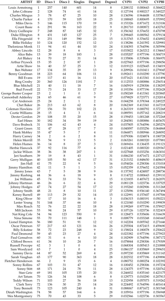
Table 3.Datasets related to the jazz artists biplex network.
ARTIST ID Discs 1 Discs 2 Singles Degree1 Degree2 CVPl1 CVPl2 CVPBI
Louis Armstrong 1 257 140 601 14 8 0.208132 0.000643 0.306822 John Coltrane 2 128 74 61 14 32 0.127194 0.900217 0.349227 Charles Mingus 3 78 47 25 10 28 0.136596 0.964608 0.337863 Charlie Parker 4 170 59 105 18 25 0.188845 0.800695 0.370992 Miles Davis 5 146 115 170 19 31 0.153326 0.871672 0.313106 Count Basie 6 291 96 163 22 9 0.281710 0.000872 0.432763 Dizzy Guillespie 7 248 87 145 32 15 0.356342 0.376652 0.470798 Duke Ellington 8 431 145 127 25 7 0.298445 0.000562 0.379134 Ella Fitzgerald 9 251 149 590 23 15 0.313765 0.376652 0.434902 Billie Holiday 10 124 120 152 12 13 0.138286 0.241592 0.329981 Thelonious Monk 11 94 61 44 10 24 0.104393 0.764596 0.305996 Abbey Lincoln 12 28 8 6 3 17 0.033822 0.263212 0.134663 Alice Babs 13 39 18 183 1 28 0.035207 0.977196 0.304719 Art Blakey 14 70 27 31 14 19 0.135806 0.535606 0.306970 Arthur Prysock 15 35 2 87 1 28 0.027843 0.977196 0.298056 Artie Shaw 16 40 37 25 3 12 0.019123 0.025645 0.134019 Ben Webster 17 134 35 29 13 9 0.209926 0.010411 0.279045 Benny Goodman 18 223 64 106 11 8 0.092611 0.010290 0.137790 Bill Evans 19 117 41 16 11 20 0.071621 0.413341 0.161494 Bing Crosby 20 360 126 1181 7 10 0.112533 0.000886 0.256514 Blue Mitchell 21 40 11 18 7 16 0.045919 0.258306 0.138295 Bud Powell 22 73 24 33 17 28 0.193356 0.977196 0.352628 George Buster Cooper 23 2 1 0 3 20 0.050249 0.413341 0.203845 Cannonball Adderley 24 65 46 61 9 27 0.079829 0.723771 0.232014 Cat Anderson 25 24 2 1 2 16 0.044258 0.378344 0.249225 Chet Baker 26 213 63 62 8 20 0.062369 0.413341 0.167218 Coleman Hawkins 27 156 70 102 21 8 0.263319 0.000792 0.372268 Cootie Williams 28 15 4 3 6 14 0.089591 0.057162 0.208219 Dexter Gordon 29 108 35 20 15 28 0.159453 1.001248 0.372268 Earl Hines 30 182 34 59 19 10 0.284581 0.000886 0.403670 Dave Brubeck 31 106 62 43 4 24 0.037805 0.764596 0.285276 Grant Green 32 47 28 17 7 10 0.040097 0.033256 0.064868 Hank Mobley 33 47 5 7 4 11 0.066871 0.000946 0.268092 Harry Carney 34 2 6 2 8 11 0.079306 0.024874 0.180728 Helen Merrill 35 54 9 13 5 2 0.063261 0.000320 0.077881 Helen Humes 36 14 8 27 3 13 0.069416 0.136435 0.191121 Herbie Hancock 37 92 116 77 4 2 0.021405 0.000320 0.029367 Jackie Wilson 38 36 38 207 1 10 0.027848 0.033256 0.063010 Jeri Southern 39 19 8 43 1 31 0.006230 0.871672 0.237127 Gerry Mulligan 40 105 50 62 17 31 0.213152 0.848650 0.408619 Jim Hall 41 75 22 9 5 16 0.054026 0.258306 0.151018 Jimmy Hamilton 42 11 5 1 3 15 0.052359 0.376652 0.243584 Jimmy Jones 43 7 5 38 9 16 0.137392 0.424007 0.288736 Jimmy Rushing 44 36 6 18 9 8 0.114722 0.000643 0.239110 Joe Williams 45 74 33 74 6 15 0.121835 0.407672 0.262070 Johnny Hartman 46 26 6 22 4 29 0.081128 1.023736 0.337525 Johnny Hodges 47 74 27 54 17 12 0.193260 0.002906 0.311268 Johnny Smith 48 21 8 10 11 27 0.125096 0.936140 0.367494 Kenny Burrell 49 113 29 32 14 15 0.122991 0.157607 0.197506 King Oliver 50 17 10 16 4 3 0.036315 0.000191 0.050221 Lester Young 51 144 37 66 10 8 0.121040 0.010290 0.199839 Max Roach 52 76 22 22 18 28 0.199269 0.977196 0.378927 Milt Jackson 53 94 24 57 10 29 0.107126 1.023736 0.322419 Nat King Cole 54 94 123 550 9 19 0.128473 0.535606 0.316639 Nina Simone 55 70 111 148 1 9 0.008779 0.033248 0.041665 Lionel Hampton 56 180 51 91 12 12 0.142204 0.005542 0.271646 Oscar Peterson 57 217 63 121 16 26 0.255504 0.872415 0.459690 Billy Eckstine 58 72 23 248 9 12 0.158024 0.180078 0.250622 Paul Desmond 59 45 23 27 4 28 0.023382 0.977196 0.275923 Paul Gonsalves 60 31 6 6 10 24 0.182909 0.764596 0.387172 Clifford Brown 61 34 10 24 7 16 0.078844 0.258306 0.179309 Russell Procope 62 3 1 0 4 11 0.068304 0.005413 0.210888 Sam Woodyard 63 7 1 0 4 25 0.086137 0.835869 0.299651 Sammy Davis 64 87 52 269 4 25 0.097230 0.835869 0.311143 Sarah Vaughan 65 177 90 363 18 28 0.202532 0.977196 0.439896 Fletcher Henderson 66 2 9 15 6 4 0.080752 0.000254 0.102392 Sonny Rollins 67 103 31 47 12 16 0.100452 0.258306 0.197234 Sonny Stitt 68 171 24 78 11 28 0.124375 0.977196 0.320762 Stan Getz 69 181 105 135 20 31 0.246832 0.835160 0.423175 Art Tatum 70 126 34 108 6 8 0.129773 0.010290 0.207813 Teddy Wilson 71 103 27 56 18 13 0.232958 0.057073 0.319262 Clark Terry 72 136 30 25 14 24 0.224492 0.764596 0.401614 Tony Bennett 73 123 105 240 8 31 0.088067 0.871672 0.301548 Dinah Washington 74 58 57 164 6 28 0.105916 0.977196 0.356948 Wes Montgomery 75 70 43 33 5 29 0.032566 1.023736 0.303567
Table3summarizes the whole set of data collected regarding to the biplex network of jazz artists of the early twentieth century. This table shows the names of the artists and their identifiers as network nodes. The following three columns show the information related to the musical production of each artist. The columndiscs1 shows the number of discs (LP’s) released commercially, the columndiscs2 shows, for each artist, the number of discs of other colleagues in which the artist has appeared and in the third columnsingleswe have the number of singles released commercially. The next columns
degree1anddegree2show the degrees of a node in the graphs of layer 1 and layer 2, respectively. Finally, the last three columns show the results of the calculated centralities. The centralityCVPl1refers to the eigenvector centrality taking individually the first layer,CVPl2refers to the eigenvector centrality taking individually the second layer, while the CVPBI centrality is shown in the third column, having been calculated running Algorithm 2.These results are analyzed and discussed in next section.
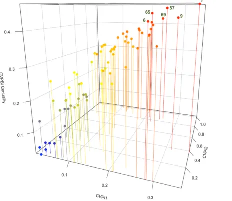
The biplex centrality for the jazz artists network is displayed in Figure10, where the biplex centrality CVPBI is represented in front of the individual centralities of each layer. Figure10shows how there is a group of nodes with very high CVPBI centrality and a low centrality in layer 2.
Figure 10.Eigenvector centrality CVPBI for jazz artists network. 4. Discussion
The way in which we calculate the centralities CVP (eigenvector centrality with data) and CVP2f (eigenvector centrality based on the two-layer PageRank approach) differs from the way in which the classical eigenvector centrality is calculated. When considering the CVP centrality it is assumed that the importance of the data associated with the node itself may be not negligible in the calculation of its importance within the network. If the expression (3) is observed, we notice the presence of the componentx, which fulfills this function precisely and which does not appear in the classical eigenvector centrality.
The importance of this detail on the computation of centrality is shown in the first network of the results section. On a simple network of 10 nodes, with two clearly differentiated components, three data sets are strategically distributed between the different nodes of the network. We analyze them briefly.
We pay attention to the upper graph corresponding to the data setD1, which centers all the data of the network in the first four nodes. Firstly, It is observed that the results of the three centralities studied are coherent, in the sense that the most relevant nodes coincide in the three measures, maintaining the order of importance of the nodes in all cases. However, certain differences are seen in the values of centrality in those nodes where the data are concentrated. Specifically, the biggest differences between the classic eigenvector centrality and the rest are given in nodes 1, 3 and 4, which are the ones that concentrate the data. This is a consequence of the way in which eigenvector centrality for networks with data is calculated, taking into account not only the degree of the node but also its own importance based on the data it contains. Observing the graphs shown in Figure4, the great similarity in the values of the CVPclassic and CVP2f centralities is clear. Likewise, when the nodes do not have data, the three measures of centrality are practically identical. In the central graph of Figure4, corresponding to datasetD2, it can be seen how the most relevant node in the network is 7, which is one of the two nodes that stores the data present in the network. One might think that the second most relevant node of the same would be node 4, which is the other node with 10 data. However, this is not the case, since the second node in importance is node 5. The reason for this behavior is that, although node 5 does not contain data, it is connected to the two nodes that contain all the data of the network (nodes 4 and 7). This case intuitively shows us the idea on which the eigenvector centrality is based.
In the lower graph of Figure4, corresponding to datasetD3, the importance of connectivity is also seen. Although nodes 1 and 7 have the maximum data, node 7 is the most relevant due to its connectivity (grade 5), compared to node 1 that only has degree 2. The nodes connected to node 7 present a higher centrality for its greater connectivity. The fact repeated is that the greatest differences in the values of the centralities occur when data are present in the nodes.
This coherence in the values of the centralities studied is not only observed in small networks. Tests have been carried out with networks of different sizes, up to 10, 000 nodes. The literature suggests different alternatives to study the correlations between two rankings; in this case a classic one has been chosen to perform the numerical tests, as it is the the Spearman correlation coefficient. The results are conclusive: in all the cases tested with different sizes, the Spearman coefficient between the variables exceeded the 0.9999 value, being 1 in most cases from sizes ofn=100. This positive correlation is very relevant in this proposal since we have a solid measure such as the CVP2f centrality that allows us to design a new measure for networks with multiple layers.
Let us consider the networkM1with two layers and 10 nodes. In the first layerl1the data are associated with the nodes with less connectivity, while in layerl2they are located in the two nodes with greatest connectivity. The influence of data on those nodes with more links is clearly observed. If we analyze the global centrality of the biplex network, it is much closer to the eigenvector centrality calculated for layerl2than for layerl1. In fact, the three most central nodes of the measures CVPl2 and CVPBI are the same, although following a different order in the ranking. However, if we consider separately the centrality of layerl1, it has nothing to do with the global results when analyzing the network by layers. In layerl1the two most relevant nodes do not coincide with the nodes that have more data; however, this does not happen in layerl2, where clearly the sum of data and degree makes the most central nodes are those that accumulate more data.
This shows that when a multilayer network with data is considered and evaluated, the results differ when the centrality is applied individually to each of the layers.
Now, we discuss the jazz musicians network described in Section3.3. Note that the goal is not only to establish a ranking of musicians of this time based on their collaborations and musical production. To address this objective, it would be enough to calculate the eigenvector centrality of layerl1(CVPl1) and we would have this classification. Note that we relate the collaborations between artists with those who are contemporary with each other. Following the idea of centrality based on the eigenvector concept, we consider that the relevance of an artist is also related to the presence of contemporary artists and, in addition, the more famous they are, the more fame they provide to a work and production. Therefore, the goal is not only to establish a ranking of musicians of that time
based on their collaborations and musical production. If this were the objective, it should be enough to calculate the CVP centrality of layer 1 and we would have this classification. In this case it is mixed the collaborations between artists with those who are contemporary with each other. Following the idea of centrality based on the eigenvector concept, it is established that the importance of an artist is also related to the presence of contemporary artists and, in addition, the more relevant they are, the more value they provide to their work and production.
A portion of the dataset collected is shown in Table3, while the geographical location of the artists’ birth places can be seen in the USA map in Figure8, where the large production of artists in the east and southeast of the country is clear.
Regarding to the data referring to the musical production, some highlights may be remarked:
• Much of the artists with the highest production of LP’s and singles are singers, such as Ella Fitzgerald, Billie Holiday, Bing Crosby, Nat King Cole, Nina Simone, Sarah Vaughan or Tony Bennett.
• It is remarkable the huge musical production of Bing Crosby.
• Most artists whose musical production is very low is a consequence of having been part of other bands, though their importance and influence in later times is undeniable.
• If we focus on the artists who have a higher number of collaborations with other musicians, most of them are part of all the lists of the best jazz musicians of all time, such as Dizzy Guillespie, Duke Ellington, Ella Fitzgerald, Miles Davis, Charlie Parker, Stan Getz or Louis Armstrong. To analyze the data obtained from the jazz artists network, Table3is simplified by taking the 15 nodes that present higher values of centralities. Therefore, Table4summarizes the ranking of nodes for the calculated values of centralities CVPl1, CVPl2 and CVPBI.
An extensive analysis of the results reproduced in Table4and displayed in Figure11is performed. As already mentioned, if we limit to the calculation of the eigenvector centrality for networks with data in layerl1using Algorithm 1, we obtain a classification of the nodes in importance according to the collaborations with other artists and taking the data of his musical production in terms of records. We must bear in mind that it is being valued as relevant not only the number of collaborations but the quality of these, always under the prism that we are relevant if our contacts are relevant. The importance of the musicians with whom they collaborate or participate is measured. Looking at Figure11(up left), the first in the ranking of the artists in the classification to measure the centrality CVPl1 is Dizzy Gillespie, key trumpeter in the evolution of jazz to the present. It is the node with the highest degree, that is, with a greater number of connections with other musicians.
It is noted that in this list are some of the best known artists of that time by the public, such as Dizzy Gillespie, Duke Ellington, Ella Fitzgerald, Count Basie, Oscar Peterson, Louis Armstrong and others. Other names are also not as well known as Earl Hines, pianist of the band of Louis Armstrong and whose musical production is remarkable with 182 albums released.
If the eigenvector centrality for layer 2 is now analyzed, a different pattern is observed. To begin with, there are hardly any names on the list that are so familiar to non-specialists in jazz music. Remark that now we relate the artists for contemporaneity. It follows that the artists with higher centrality are those born between 1923 and 1924, years of abundance in the birth of artists of unquestionable quality, some of whom are on this list. It is not surprising that several artists have the same centrality, since they were born in the same year they form similar subgraphs with the same degrees. Figure11 (up right) displays the 15 first names in the classification.
Table 4.The first 15 jazz artists with higher centralities.
Ranking CVPl1 Artist CVPl2 Artist CVPBI Artist
1 0.3563 Dizzy Guillespie 1.0237 Johnny Hartman 0.4708 Dizzy Guillespie 2 0.3138 Ella Fitzgerald 1.0237 Milt Jackson 0.4597 Oscar Peterson 3 0.2984 Duke Ellington 1.0237 Wes Montgomery 0.4399 Sarah Vaughan 4 0.2846 Earl Hines 1.0012 Dexter Gordon 0.4349 Ella Fitzgerald 5 0.2817 Count Basie 0.9772 Alice Babs 0.4328 Count Basie 6 0.2633 Coleman Hawkins 0.9772 Arthur Prysuck 0.4232 Stan Getz 7 0.2555 Oscar Peterson 0.9772 Bud Powell 0.4086 Gerry Mulligan 8 0.2468 Stan Getz 0.9772 Max Roach 0.40367 Earl Hines 9 0.2330 Teddy Wilson 0.9772 Paul Desmond 0.4016 Clark Terry 10 0.2245 Clark Terry 0.9772 Sarah Vaughan 0.3872 Paul Gonsalves 11 0.2132 Gerry Mulligan 0.9772 Sonny Stitt 0.3791 Duke Ellington 12 0.2099 Ben Webster 0.9772 Dinah Washington 0.3789 Max Roach 13 0.2081 Louis Armstrong 0.9646 Charles Mingus 0.3723 Coleman Hawkins 14 0.2052 Sarah Vaughan 0.9361 Johnny Smith 0.3722 Dexter Gordon 15 0.1993 Max Roach 0.9002 John Coltrane 0.3710 Charlie Parker
Figure 11.Jazz network centralities CVPl1 (upper left), CVPl2(upper right), and CVPBI taking the top 15 nodes (musicians) in the ranking of centralities.
Considering the network as a whole and not individually by layers, the influences of the different relationships between the nodes and the data associated with them are mixed together and the layers interact. Applying Algorithm 2 a ranking is obtained (see Figure11down).The winner is Dizzy Gillespie, a trumpet virtuoso and improviser. In the 1940s Gillespie, with Charlie Parker, became a major figure in the development of bebop and modern jazz. The second artist in the classification is
Oscar Peterson, exceptional pianist in the history of music. Being born in 1925, being contemporary of many jazz greats with whom he has collaborated actively throughout his career and his extensive musical production of both albums and singles takes to occupy a high position in this ranking. In the third place appears Sarah Vaughan, born in 1924. As in the previous case, her enormous musical production and having sung with the most relevant artists in the history of jazz cause her to be in second place. The same behavior repeats with the rest of the artists.
If we compare the three classifications, the names do not match. This is really what we expected when we consider multipex networks: the value of individual centrality does not exactly match the global centrality.
This example help us to understand how the data must be analyzed in the context of the networks and their characteristics. Thus, the analysis of the data collected on the musical production shows us a clear pattern as it is that the singers of this list have a very high musical production. The most obvious cases are those of Bing Crosby, Ella Fitzgerald or Nat King Cole, which have a singles production of 1181, 590 and 550, respectively, occupying the first three positions if we take this isolated data. Note that these artists are born before 1919 and the great explosion of artists in those decades is between 1921 and 1927, which penalizes them and it does not allow them to occupy higher positions in the rankings. Throughout the example, we see the possibilities of treatment that a dataset has from the study of diverse relations between the different nodes of the network. If we had related the artists in another sense, the results probably would not be same, but it is certain that in the final list some of the greatest artists in jazz history should appear.
5. Conclusions
In this paper, a centrality measure for biplex networks (CVPBI), based on the eigenvector centrality for networks with data, has been designed and implemented. The advantage of this type of measure is twofold. Firstly, it can determine the importance of the nodes of a network by analysing multiple relationships between the nodes. On the other hand, it allows to work with several datasets associated with the nodes themselves.
As a preliminary step to the design of the measure for multilayer networks, it has been necessary to adapt the eigenvector centrality for networks with data to the idea underlying the two-layered approach PageRank. Following this technique, a new centrality (CVP2f) is designed by means of the construction of a 2×2 block matrix, where the blocks of the main diagonal have the objective of separating the effect of the network topology on the data with the quantity of these. Thus, the first block assumes the importance of the network topology while the second block takes into account the influence of the data at a global or residual level.
In the several numerical tests performed on networks of different types and sizes, a coherence was observed in the values offered by CVP2f measure with the classic eigenvector centrality (CVPclassic) and with the eigenvector centrality for networks with data (CVP). This consistent result has allowed us to generalize to multiplex networks the idea of considering blocks in each of the layers differentiating the influence of the data according to the network topology and the data as a whole (following a similar reasoning as in the CVP2f centrality).
The centrality proposed for multiplex networks has been experienced on a real network of jazz musicians of the early twentieth century. It has demonstrated its ability to evaluate different relationships on the same set of nodes when different datasets are considered. From this particular example, we have shown how introducing a layer structure, by distinguishing different types of interactions between the nodes, may vary the behaviour of the network.
Author Contributions:All authors contributed equally to: conceptualization, F.P., L.T. and J.F.V.; methodology, F.P., L.T. and J.F.V.; formal analysis, F.P., L.T. and J.F.V.; investigation, F.P., L.T. and J.F.V.; writing—original draft preparation, F.P., L.T. and J.F.V.
Funding: This research is partially supported by the Spanish Government, Ministerio de Economía y Competividad, grant number TIN2017-84821-P.
Conflicts of Interest:The authors declare no conflict of interest. Abbreviations
The following abbreviations are used in this manuscript: CVP Eigenvector centrality for networks with data
CVPclassic Eigenvector centrality for networks with data with classic centrality calculation CVP2f Eigenvector centraliy using two-layer approach PageRank
CVPBI Eigenvector centrality for biplex networks CVPM Eigenvector centrality for multiplex networks
CVPl1 Eigenvector centrality for networks with data for layerl1
CVPl2 Eigenvector centrality for networks with data for layerl2 References
1. Estrada, E. The Structura of Complex Networks. Theory and Applications; Oxford University Press: Oxford, UK, 2012.
2. De Domenico, M.; Granell, C.; Porter, M.; Arenas, A. The physics of spreading processes in multilayer networks. Nat. Phys.2016,12, 901–906. [CrossRef]
3. De Domenico, M.; Solé-Ribalta, A.; Cozzo, E.; Kivelä, M.; Moreno, Y.; Porter, M.; Gómez, S.; Arenas, A. Mathematical formulation of multilayer networks. Phys. Rev. X2013,3, 041022. [CrossRef]
4. Kivela, M.; Arenas, A.; Barthelemy, M.; Gleeson, J.; Moreno, Y.; Porter, M. Multilayer networks.
J. Complex Netw.2014,2, 203–271. [CrossRef]
5. Padgett, J.; Ansell, C. Robust Action and the Rise of the Medici. Am. J. Soc.2016,98, 1259–1319. [CrossRef] 6. Cellai, D.; Bianconi, G. Multiplex networks with heterogeneous activities of the nodes. Phys. Rev. E2016,
93, 032302. [CrossRef] [PubMed]
7. De Domenico, M.; Solè-Ribalta, A.; Gómez, S.; Arenas, A. Navigability of interconnected networks under random failures. Proc. Natl. Acad. Sci. USA2014,111, 8351–8356. [CrossRef] [PubMed]
8. Cozzo, E.; Arruda, G.; Rodrigues, F.; Moreno, Y.Multiplex Networks. Basic Formalism and Structural Properties; Springer: Berlin/Heidelberg, Germany, 2018.
9. Cardillo, A.; Gómez-Gardeñes, A.; Zanin, M.; Romance, M.; Papo, D.; del Pozo, F.; Boccaletti, S. Emergence of network features from multiplexity.SIAM Rev.2013,3, 1–122. [CrossRef] [PubMed]
10. De Domenico, M.; Lancichinetti, A.; Arenas, A.; Rosvall, M. Identifying modular flows on multilayer networks reveals highly overlapping organization in interconnected systems. Phys. Rev. X2015,5, 011027. [CrossRef]
11. Battiston, S.; Caldarelli, G.; May, R.; Roukny, T.; Stiglitz, J. The price of complexity in financial networks.
Proc. Natl. Acad. Sci. USA2016,113, 10031–10036. [CrossRef]
12. Bentley, B.; Branicky, R.; Barnes, C.; Chew, Y.; Yemini, E.; Bullmore, E.; Vértes, P. The Multilayer Connectome of Caenorhabditis elegans.PLoS Comput. Biol.2016,12, e1005283. [CrossRef]
13. Sola, L.; Romance, M.; Criado, R.; Flores, J.; Garcia del Amo, A.; Boccaletti, S. Eigenvector centrality of nodes in multiplex networks. Chaos2013,23, 033131. [CrossRef]
14. Iacovacci, J.; Rahmede, C.; Arenas, A.; Bianconi, G. Functional Multiplex PageRank. arXiv 2016, arXiv:1608.06328v2.
15. Halu, A.; Mondragón, R.; Panzarasa, P.; Bianconi, G. Multiplex PageRank. PLoS ONE2013,8, e78293. 16. Solé-Ribalta, A.; De Domenico, M.; Gómez, S.; Arenas, A. Centrality Rankings in Multiplex Networks.
In Proceedings of the 2014 ACM Conference on Web Science, Bloomington, IN, USA, 23–26 June 2014; ACM: New York, NY, USA, 2014; pp. 149–155. [CrossRef]
17. Spatocco, C.; D’Andrea, A.; Domeniconi, C.; Stilo, G. A New Framework for Centrality Measures in Multiplex Networks. arXiv2018, arXiv:1801.08026.
18. Pedroche, F.; Romance, M.; Criado, R. A biplex approach to PageRank centrality: From classic to multiplex networks. Chaos2016,26, 065301.
19. Agryzkov, T.; Curado, M.; Pedroche, F.; Tortosa, L.; Vicent, J.F. Extending the Adapted PageRank Algorithm Centrality to Multiplex Networks with Data Using the PageRank Two-Layer Approach. Symmetry2019,
11, 284. [CrossRef]
20. Agryzkov, T.; Tortosa, L.; Vicent, J.; Wilson, R. A centrality measure for urban networks based on the eigenvector centrality concept.Environ. Plan. B2017,291, 14–29. [CrossRef]
21. Arruda, G.; Cozzo, E.; Peixoto, T.; Rodrigues, F.; Moreno, Y. Disease Localization in Multilayer Networks.
Phys. Rev. X2017,7, 011014. [CrossRef]
22. Bobadilla, J.; Ortega, F.; Hernando, A.; Gutiérrez, A. Recommender systems survey. Knowl.-Based Syst.2013,
46, 109–132. [CrossRef]
23. Stai, E.; Kafetzoglou, S.; Tsiropoulou, E.E.; Papavassiliou, S. A Holistic Approach for Personalization, Relevance Feedback & Recommendation in Enriched Multimedia Content. Multimed. Tools Appl. 2018,
77, 283–326. [CrossRef]
24. Rabieekenari, L.; Sayrafian, K.; Baras, J. Autonomous relocation strategies for cells on wheels in environments with prohibited areas. In Proceedings of the 2017 IEEE International Conference on Communications (ICC), Paris, France, 21–25 May 2017; pp. 1–6. [CrossRef]
25. Tsiropoulou, E.; Koukas, K.; Papavassiliou, S. A Socio-physical and Mobility-Aware Coalition Formation Mechanism in Public Safety Networks.EAI Endorsed Trans. Future Int.2018,4, 154176. [CrossRef]
26. Bonacich, P. Power and centrality: A family of measures. Am. J. Soc.1987,92, 1170–1182. [CrossRef] 27. Horn, R.; Johnson, C.Topics in Matrix Analysis; Cambridge University Press: New York, NY, USA, 1991. 28. Team, R.C.R: A Language and Environment for Statistical Computing; R Foundation for Statistical Computing:
Vienna, Austria, 2013. c
2019 by the authors. Licensee MDPI, Basel, Switzerland. This article is an open access article distributed under the terms and conditions of the Creative Commons Attribution (CC BY) license (http://creativecommons.org/licenses/by/4.0/).
![Figure 1 shows a schematic representation of the eigenvector centrality model proposed in [20]](https://thumb-us.123doks.com/thumbv2/123dok_us/893534.2614830/5.892.177.713.287.645/figure-shows-schematic-representation-eigenvector-centrality-model-proposed.webp)