1 INTRODUCTION
The EWASE project (Effectiveness and Efficiency of Early Warning Systems for flash-floods) is a R&D project within the ERA-NET CRUE integrated project. For the evaluation of early warnings systems (EWS) effectiveness and efficiency two important aspects have to be addressed: the reliability of the warning and the damage prevented by the warning. Within EWASE, we define the effectiveness of an Early Warning with respect to the reliability of the forecast, and we define its efficiency with respect to the economic benefit of the forecast.
In an efficient EWS the flood alert has to be bal-anced with respect to both factors because the pro-longation of the warning lead time may on the one hand increase the benefit of the alert but on the other hand comes along with a decrease of forecast reli-ability. In this context, it is important to take into ac-count that a successful warning will bring about (socio-) economic benefit whereas a false alert leads to (socio-) economic loss.
This paper discusses the aspect of EWS effec-tiveness in terms of an evaluation of forecast reli-ability. A companion paper (Gocht et al. 2008) ad-dresses the economic aspects related to the efficiency of EWS.
EWASE develops its approach on the basis of two medium sized river basins prone to flash floods: The Besòs basin (1020 km²), in a Mediterranean climate, near Barcelona, Spain, and the Traisen
ba-sin (921 km²), with an alpine climate, in Lower Aus-tria.
2 OBJECTIVES
The motive of flood warning is to reduce damages by taking preventive measures. Hence, an effective warning system provides reliable forecasts suffi-ciently in advance to realize the according actions. Obviously, the required lead time depends on the specific tasks to be completed and, as a conse-quence, it is variable for the different stakeholders and objects at risk.
In flash-flood prone areas critical situations de-velop quickly and put high demands on the warning lead time (Anquetin, et al. 2004). Flood warning based on observations of upstream river gauges only capitalizes on the travel times in the water course and thus most often is insufficient in this respect. In-stead, the application of advanced technologies is required. In this context, the use of rainfall runoff models is mandatory in order to extend the lead time which then starts from the moment rainfall is ob-served. Still, the gain of time is limited approxi-mately to the response time of the basin. A further increase of the forecast lead time can only be achieved by including quantitative precipitation forecasts (QPF). Radar nowcasting is a promising technique for the short term anticipation of rainfall (Wilson, et al. 1998). However, these procedures
EWASE - Early Warning Systems Efficiency: Evaluation of flood
forecast reliability
K. Schröter & M. Ostrowski
IHWB. TU-Darmstadt, Germany
M. Gocht
Water&Fincance, Berlin Germany
B. Kahl & H.-P. Nachtnebel
IWHW, BOKU Wien, Vienna, Austria
C. Corral & D. Sempere-Torres
GRAHI-UPC, Barcelona, Spain
ABSTRACT: Effective flood warning requires that reliable flood forecasts are available sufficiently in ad-vance in order to realize preventive measures. A methodology is proposed to evaluate forecast reliability as a function of lead time. The approach is based on the assumption that forecast reliability can be approximately described by a statistical analysis of the prediction errors available from past flood events. In this context, un-certainties associated with QPF and hydrological modeling are explicitly addressed via an ensemble modeling approach. The procedure is applied to two operational early warning systems in meso-scale river basins prone to flash floods. The results emphasize that the importance of quantitative precipitation forecasts increases in relative comparison to the predictive performance of the hydrological model as lead time is extended. The presentation of forecast reliability as a function of lead time provides a possibility to include this information in the decision about an alert for improved warning.
provide useful information at the best two hours in advance. Beyond, QPF based on numerical weather prediction (NWP) models can be used to extend the flood forecast up to several days, yet with less accu-racy as lead time extends (Collier 2007, Yates, et al. 2000).
Both the application of hydrological models and in particular the use of QPF information brings about considerable uncertainties concerning the flood forecast and the warning. In view of these un-certainties, the capability to reliably predict floods is determined by the anticipation and provision of ac-curate rainfall information in space and time (Yates, et al. 2001) as well as by the correct reproduction of the hydrological system in terms of the state and the dynamic behavior by means of the hydrological simulation model.
Therefore, to evaluate whether or not an EWS is effective the reliability of the flood forecasts has to be quantified as a function of the lead time in view of the relevant sources of uncertainty in the forecast-ing chain. Further, it has to be discussed in view of the intended purpose of the warning and the required time to complete the preventive measures.
Given this background, the objective of this work is to develop a practicable approach to assess the flood forecast reliability of EWS. This provides im-portant information concerning the effectiveness and efficiency of EWS within the context of a risk based evaluation of structural and non structural flood risk management measures.
3 METHODOLOGY
Basically, the objective of hydrological forecasting is to provide quantitative information about the fu-ture evolution of discharges or water levels. In this regard, flood forecasts support the decision on flood alerts in EWS operation. However, the prediction of future events is always uncertain owing to the vari-ability inherent to natural processes and, more im-portantly, owing to limited knowledge about the fu-ture development of meteorological conditions as well as the state and the dynamic behavior of the hydrological system. In particular, the uncertainty concerning the predicted flood event exists with re-gard to the magnitude, the location and the timing of the expected flood peak. In this context, Krzysztofowicz (1999) and Todini (2007) pointed out, that the term predictive uncertainty refers to the actual values of the predicted variable.
In the case of model based forecasting systems using QPF the predictive uncertainty is conditional on the hydrological model applied, which represents the available knowledge about the hydrological sys-tem, and on the capability of the QPF method to an-ticipate the characteristics of forthcoming storms. Thus, predictive uncertainty characterizes the state
of knowledge about the forecasted variable and is a function of the uncertainties in the data and the re-production of the natural system with a simulation model.
In theory, predictive uncertainty can be expressed in terms of a probability distribution function that describes the variation and the expected value of the predicted variable. Todini (2007) illustrates how this distribution function can be inferred from the com-parison of predicted and observed values using a Bayesian approach. However, practical approaches to determine the distribution function accounting for all sources of predictive uncertainty are still under evaluation (Krzysztofowicz 2001, Krzysztofowicz & Maranzano 2004).
Therefore, the approach proposed within this work is based on the assumption that the predictive uncertainty can be approximated by the errors be-tween predicted and observed discharge values. To this end, the capability of a flood forecasting system to predict discharges is evaluated on the basis of available observations from past events in terms of a statistical analysis of the prediction error defined in Equation 1. i Qobs i Qobs i Qsim i − = τ τ ε , , (1)
Where εi,τ denotes the prediction error at time
step i of the event associated with a specific forecast lead time τ. The error is calculated for each time step i of the period analyzed as the absolute difference between the simulated discharge value for this point of time predicted with lead time τ (Qsimi,τ ) - i.e.
which is produced at i-τ - and the discharge actually observed at this time step (Qobsi) normalized with Qobsi.
The prediction error εi, τ is the outcome of the
dif-ferent sources of uncertainty in the flood forecasting chain. In the ideal case of a perfect forecast the pre-diction would exactly match the observation of the real world discharge (within the range of the effec-tive observational error).
From the analysis of equation 1 for one event or a set of flood events a sample of errors is obtained. Assuming that all error values stem from the same population this sample is statistically summarized in terms of a probability density function (PDF) or a cumulative distribution function (CDF) respectively. The CDF allows extracting the probabilities of hav-ing errors within a certain range. On this note, the evaluation of the CDF for a particular probability quantile provides an estimate of the magnitude of the prediction error with the according level of con-fidence. In line with this interpretation, the error at the 85% percentile of the CDF (εi,τ(85%)) is
as-sumed to provide an appropriate estimate of forecast reliability. As reliability is usually defined on a scale between zero (unreliable) and one (reliable)
εi,τ(85%) is inversely related to forecast reliability (FR) as in equation 2. 0 : %) 85 ( , 1− ≥ = i FR FR ε τ (2)
According to this, forecasts with small prediction errors are more reliable than forecasts with large er-rors.
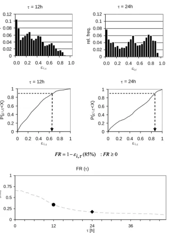
For illustration, the procedure of statistical analy-sis and evaluation of forecast reliability is exempli-fied in Figure 1. The PDF and corresponding CDF for error samples obtained for different lead times τ
are shown as well as the dependence of FR on the lead time.
Within this framework the dependence of FR on the forecast lead time is examined by evaluating equation 1 for hydrographs that are predicted with different lead times τ. To this end, a multiple step ahead forecast approach (WMO 1992) is carried out. This includes the generation of forecasted hydro-graphs for multiple time steps ti (i=1,…n) of an event using different lead time periods τ (τ = +1,…,+p [h]). Hydrographs are simulated using ob-served rainfall until ti and the precipitation forecast available at ti. The corresponding sample of εi,τ
re-flects the predictive performance of the forecasting system throughout the analyzed period.
τ = 24h 0 0.2 0.4 0.6 0.8 1 0 0.2 0.4 0.6 0.8 1 εi,τ P(ε i ,τ <X ) τ = 12h 0 0.02 0.04 0.06 0.08 0.1 0.12 0.0 0.2 0.4 0.6 0.8 1.0 εi,τ re l. fr e q . τ = 24h 0 0.02 0.04 0.06 0.08 0.1 0.12 0.0 0.2 0.4 0.6 0.8 1.0 εi,τ re l. f re q . FR (τ) 0 0.25 0.5 0.75 1 0 12 24 36 τ [h] FR (0. 8 5) 0 : %) 85 ( , 1− ≥ = i FR FR ε τ τ = 12h 0 0.2 0.4 0.6 0.8 1 0 0.2 0.4 0.6 0.8 1 εi,τ P( ε i ,τ <X ) τ = 24h 0 0.2 0.4 0.6 0.8 1 0 0.2 0.4 0.6 0.8 1 εi,τ P(ε i ,τ <X ) τ = 24h 0 0.2 0.4 0.6 0.8 1 0 0.2 0.4 0.6 0.8 1 εi,τ P(ε i ,τ <X ) τ = 12h 0 0.02 0.04 0.06 0.08 0.1 0.12 0.0 0.2 0.4 0.6 0.8 1.0 εi,τ re l. fr e q . τ = 24h 0 0.02 0.04 0.06 0.08 0.1 0.12 0.0 0.2 0.4 0.6 0.8 1.0 εi,τ re l. f re q . FR (τ) 0 0.25 0.5 0.75 1 0 12 24 36 τ [h] FR (0. 8 5) 0 : %) 85 ( , 1− ≥ = i FR FR ε τ τ = 12h 0 0.2 0.4 0.6 0.8 1 0 0.2 0.4 0.6 0.8 1 εi,τ P( ε i ,τ <X ) τ = 12h 0 0.2 0.4 0.6 0.8 1 0 0.2 0.4 0.6 0.8 1 εi,τ P( ε i ,τ <X )
Figure 1. Procedure for the statistical analysis of prediction
er-rors εi,τ and evaluation of forecast reliability. Above the PDF of
error samples for τ = +12h and τ = +24h are shown. In the
middle the corresponding CDF are plotted. Below the
interpre-tation of εi,τ(85%) in terms of FR and its dependence on τ is
exemplified.
It has to be recalled that the sample of errors εi,τ is
conditional on the QPF and the simulation model used for the generation of flood forecasts. Assuming that the uncertainties associated with the QPF and with the hydrological model considerably contribute to the reliability of the forecast, it is worthwhile to address these uncertainty sources more directly in order to obtain a more complete picture of predictive uncertainty. In this respect, ensemble modeling is a promising approach to explicitly incorporate these sources of uncertainty in the evaluation of FR.
The basic idea of ensemble modeling in natural sciences is to consider a set of different possible re-alizations of future conditions. In Meteorology, one method to obtain an ensemble is to introduce ran-dom perturbations to the initial state of a meteoro-logical model (Lorenz 1963). In that way a set of possible future developments of meteorological states and resulting precipitation fields is generated, which describes the uncertainty inherent to the pre-diction, e.g. (Buizza, et al. 1999) for NWP models and (Bowler, et al. 2006) for probabilistic radar nowcasts.
The idea of ensemble modeling can also be trans-ferred to the application of different simulation models. Every model is an interpretation of reality and relies on a scientific hypothesis about the cause-effect relations of the system under study. Therefore, the prediction of one specific model represents only one realization of all possible predictions. In view of the fact that no model outperforms all other models all the time, it is expected that the combination of different models in a multi-model ensemble repre-sents an estimation of the uncertainty related to the simulation model (Clemen 1989, Shamseldin, et al. 1997). Observed discharges Forecast reliability comparison τ εi, statistical analysis Ensemble QPF Hydrological model ensemble Flood forecast ensemble Observed discharges Forecast reliability comparison τ εi, statistical analysis Observed discharges Observed discharges Forecast reliability Forecast reliability comparison τ εi,τ εi, statistical analysis Ensemble QPF Ensemble QPF Hydrological model ensemble Hydrological model ensemble Hydrological model ensemble Flood forecast ensemble Flood forecast ensemble
Figure 2. Outline of the methodology for the analysis of fore-cast reliability using ensemble QPF and multiple hydrological models.
Within the scope of this work, following the rea-soning of Georgakakos, et al. (2004), Refsgaard, et al. (2006) the concept of multi-model ensembles is applied to characterize hydrological uncertainty.
In brief, the approach proposed to assess the fore-cast reliability of EWS is based on the statistical analysis of the prediction errors calculated according to equation 1. The sample of errors results from the evaluation of hydrographs which are determined by cascading the ensemble QPF through a set of hydro-logical models, as illustrated in Figure 2.
4 CASE STUDY
Within the scope of the EWASE project two pilot basins are considered. The first is the Traisen basin in Lower Austria. The second is the basin of the river Besòs near Barcelona (Spain).
4.1 Traisen basin
The Traisen basin is located approx. 50 km West of Vienna and discharges to the Donau river, see Fig-ure 3. The size of the catchment is 921 km² and ele-vations range from 200 m in the North to 1800 m a.s.l. in the South. In direct relation to this the cli-mate changes north-south from pannonian to alpine climate. The geology of the basin is classified into three major zones, namely the Molasse and Flysch zones and northern limestone Alps. Mean annual precipitation ranges from 600 to 1500 mm/a with maximum precipitations in summer mostly in the al-pine part.
Figure 3. Traisen river basin topography and observational network
During winter considerable amounts of snow are ac-cumulated in the southern part. The flow regime is characterized as pluvio-nival. In spring snow driven floods occur often in combination with rainfall. In summer flood events usually are caused by heavy rainfall. In particular the summer flood events are characterized by response times of 8 to 24 hours at Windpassing (cf. Figure 3). However, depending on the spatial characteristics and the location of rainfall within the basin flash-floods may occur especially in the mountainous sub-basins in the southern part.
The operational warning system for the Traisen is based on the continuous hydrological model COSERO (Kling 2002, Nachtnebel&Kahl 2007). It incorporates QPF from the INCA-System (Inte-grated Nowcasting through Comprehensive Analy-sis) (Haiden, et al. 2007), which is made available by the Central Institute for Meteorology and Geody-namics (ZAMG). INCA is based on a weighted combination of extrapolations from rain gauges and radar observations using motion vectors (nowcasts) with QPF from the NWP models ALADIN (Wang, et al. 2006) and ECMWF. Within INCA a determi-nistic QPF and an ensemble QPF are produced. The generation of the ensemble forecast is based on a random combination of the ECMWF ensembles with a pseudo ensemble of the deterministic ALADIN forecast. This ensemble is produced by shifting the QPF field on a random space lag. The nowcast data do not include a quantification of uncertainty in terms of an ensemble. Therefore for short lead times (τ < +2 h), where the nowcast data provide the es-sential part of information, all ensemble members are identical (Komma, et al. 2007).
For flood warning additional information is pro-vided by the hydrological services’ observation net-work which consists of ten rain gauges and seven online river gauges. The outcomes of the flood fore-casting system are passed on to the Warning Alert Centre (LWZ) which decides about an alert on the basis of predefined warning levels corresponding to thresholds of discharge values.
The data provided for this study comprise the de-terministic QPF and ensemble QPF with 50 mem-bers for a maximum lead time of τmax = +48 h. The forecasted precipitation fields have a spatial resolu-tion of 10 km², a temporal resoluresolu-tion of 15 minutes and are updated every hour.
4.2 Besòs basin
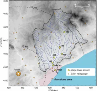
The basin of the river Besòs is situated North of Barcelona and crosses the metropolitan area before it discharges into the Mediterranean Sea, see Figure 4.
The basin area is approx. 1020 km² and shows a pronounced relief shaped by the littoral and pre-littoral mountain ranges with elevations up to 1350 m a.s.l. and steep slopes. As indicated by topography the geology of the area is differentiated between the mountain ranges, mainly composed of granites, shale, limestone and sandstone, and the central val-ley where deposits of clay, sand and conglomerate dominate (Corral 2004). In particular the area in the central valley has experienced a continuous change of land use towards extended urbanized areas and cropland which has induced an increase of runoff coefficients. According to the Mediterranean climate most part of mean annual precipitation of 660 mm/a is typically accumulated during short but intense rainfall events in particular in autumn. All these fac-tors (topography, climate and land use) bring about a very irregular and torrential flow regime with low flows of few cubic meters per second and pro-nounced peak discharges up to 2000 m²/s to 2500 m²/s which develop within response times of less than 6 h.
Flood warning in the Besòs basin is in the re-sponsibility of the Catalan water agency (ACA). At present, alerts are issued on the basis of rainfall thresholds using information from meteorological forecasts and the observational network of rain gauges and radars.
In addition, there is a separate flood alert system for the Besòs riverside park located in the down-stream reach inside the municipal area of Barcelona. The park has been created for recreational purposes to improve the quality of life in this highly urban-ized area. The aim of the EWS is to inform the peo-ple in the park about the current level of flood risk and, if necessary, to evacuate the park.
This system is operated by the sewer operation company of Barcelona (CLABSA). It uses informa-tion from the real time monitoring system (SAIH) of ACA including rain gauges, and river gauges as well as observations from the meteorological radars of the Spanish (INM) and Catalan (METEOCAT) me-teorological services.
Figure 4. Besòs river basin, topography and observational net-work
On the basis of these data discharges are continu-ously forecasted using three hydrological simulation models, including DICHITOP (Corral 2004). The decision about an alert is based on rainfall observa-tions exceeding a predefined threshold and/or a hy-drological model prediction indicating flooding of the park.
The incorporation of short term QPF using radar nowcasts is still under evaluation (Berenguer, et al. 2005). Therefore, the data available for this study consist of radar based quantitative precipitation es-timates (QPE) with a spatial resolution of 1 km² and 10 minute intervals..
4.3 Hydrological models
The hydrological multi-model ensemble is con-ceived to combine the predictions of different mod-els in order to account for the hydrological uncer-tainty in the forecasting system. Within EWASE the multi-model ensemble consists of two continuous (COSERO and WBrM) and one event based model (DICHITOP).
COSERO (Kling 2002, Nachtnebel&Kahl 2007) is a semi-distributed deterministic conceptual rain-fall runoff model developed on the basis of the HBV Model (Bergstrom 1992, Bergstrom 1995). The spa-tial representation of the catchment uses hydrologi-cal response units which are defined according to land cover, soil and height. The transformation of the flood wave along the river course can be repre-sented either by a linear reservoir or a cascade of lin-ear reservoirs.
WBrM (Lempert 2000) is a distributed determi-nistic hydrological model based on a detailed repre-sentation of soil moisture related processes. The catchment is discretised in square grids. These raster elements are the smallest unit to represent spatial heterogeneity of catchment characteristics and me-teorological input data. For each raster element vertical and lateral process rates are determined based on a piecewise linear approximation of the
a piecewise linear approximation of the process equations using conceptual approaches (Ostrowski 1991). WBrM uses a kinematic wave approach for flood routing.
DICHITOP (Corral 2004) is a conceptual distrib-uted deterministic rainfall runoff model. Grid cells form the response units for hydrological processes. Runoff generation is described using the TOP-MODEL approach (Beven & Kirkby 1979) for rural areas and the SCS method (Mockus 1957) for urban areas. Flood routing is modeled using a diffusive wave unit hydrograph for each cell which are line-arly superimposed at the basin outlet.
4.4 Events
The calibration and validation of the hydrological models has been carried out on the basis of available observations for a selection of past flood events (10 events in the Traisen basin, 13 events in Besòs ba-sin). For the testing of the method proposed a sub set of these events with different magnitudes has been used. The characteristics of these events are summa-rized in Table 1.
In view of the focus of the EWASE project on flash-floods, for the Traisen basin only summer rain events have been selected. In the Besòs basin two events, representative for convective and stratiform systems have been singled out for the study.
The start and end date indicated refer to the pe-riod considered for the evaluation of FR which cov-ers the essential part of the flood event. The sample size of prediction errors obtained for different lead times should be similar. Therefore, the earliest pos-sible start date of the period analyzed is the duration of the maximum forecast lead time applied (+τmax [h]) after the first available forecast.
Table 1. Survey of event characteristics examined for the evaluation of forecast reliability in the Traisen and the Besós basin Events Traisen C1 C4 V5 Start 3.6.04 00:00 7.8.06 00:00 3.6.06 01:00 End 5.6.04 23:00 8.8.06 23:00 4.6.06 23:00 accMAP [mm] 69 164 122
Event type Summer rain Summer rain Summer
rain
Ini. Cond. Dry Wet Wet
Runoff coef. [-] 0.16 0.22 0.25 Peak [m³/s] 82 442 340 Return period [a] 1 10-30 5 start Rising limp 3.6.04 17:00 7.8.06 03:00 2.6.06 20:00 Time to peak [h] 11 20 16 NSE*(WBrM) 0.68 0.96 0.89 NSE*(COSERO) 0.82 0.97 0.92 Besòs C2 V1 Start 19.7.01 05:00 15.1.01 05:00 End 20.7.01 12:00 16.1.01 12:00 accMAP [mm] 21 43
Event type Conv./Strat Strat.
Ini. cond. Dry Wet
Runoff coef. [-] 0.06 0.11 Peak [m³/s] 78 103 start Rising limp 19.7.01 08:00 15.1.01 17:00 Time to peak [h] 4 6 NSE* 0.89 0.69 *Nash-Sutcliffe-Efficiency (Nash & Sutcliffe 1970) achieved in the reproduction of the flood event with the hydrological model using observed precipitation
5 RESULTS
There are considerable differences concerning the characteristics of the study basins and the complex-ity of the operational EWS. As a major difference in the Besòs basin no QPF are used to drive the hydro-logical models for flood forecasting. For that reason, the methodology proposed cannot be applied to both case studies in the same detail but is adapted to the information available in each case.
The results presented in the following are based on simulations with two hydrological models in the Traisen basin and one hydrological model in the Besòs basin.
In detail, in the Traisen basin the sample of pre-diction errors εi, τ results from the evaluation of
pre-dicted hydrographs based on either the deterministic QPF or the ensemble QPF (50 members) updated hourly with a maximum forecast horizon of τmax= +48 h, which are processed with the models COSERO and WBrM. The errors are calculated at the gauging station in Windpassing (cf. Figure 3) for hourly intervals within the examined period of the events C1, C4 and V5 (cf. Table 1).
For the Besòs no QPF are applied. Instead, flood forecasts are calculated using real time available QPE from the INM radar at Corbera de Llobregat. The examined flood forecast horizon has been lim-ited to τmax= +5 h. Prediction errors εi, τ are
evalu-ated at the gauging MOCA (cf. Figure 4) for 10 minute intervals throughout the events C1 and V1 (cf. Table 1). For this study, only the results of the model WBrM are available.
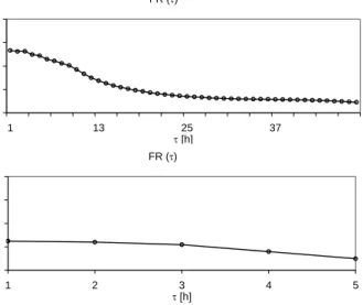
The results of the analysis are presented in Figure 5. The diagrams show the evolution of FR as a func-tion of τ for each basin resulting from the statistical analysis of the εi, τ samples as detailed above. From
the graphs a decrease of FR with increasing lead time can be noticed.
For the Traisen basin (Fig. 5 above) at best a forecast reliability of 66% is achieved. This level stays more or less constant for lead times up to τ = +4 h. Then a continuous decrease of FR can be
ob-served. The intensity of this decline is most pro-nounced for the range between τ = +4 h and τ = +15 h lead time.
The results for the Besòs (Fig. 5 below) indicate a low reliability of the flood forecasts. Even for lead times of τ = +1 h FR is only about 30% and then for
τ > +2 h continuously decreases.
These results show that the predictability of floods is limited and involves a considerable degree of uncertainty that increases with lead time. Yet, on the basis of these results it is problematic to con-clude a clear statement concerning the effectiveness of the EWS. Such evaluation would require that a threshold for the tolerated level of FR is defined. This definition is highly subjective and largely de-pends on the context of a specific decision situation. In addition, to draw any conclusions the results should be sufficiently representative of the EWS ex-amined. FR (τ) 0 0.25 0.5 0.75 1 1 13 25 37 τ [h] FR (0.85) FR (τ) 0 0.25 0.5 0.75 1 1 2 3 4 5 τ [h] FR (0 .85) FR (τ) 0 0.25 0.5 0.75 1 1 13 25 37 τ [h] FR (0.85) FR (τ) 0 0.25 0.5 0.75 1 1 2 3 4 5 τ [h] FR (0 .85)
Figure 5. Forecast reliability as a function of lead time τ for the
EWS in the Traisen basin (above) and the Besòs basin (below).
In this respect, the results presented in Figure 5 are the outcome of an aggregated evaluation of FR on the basis of several events. For the appraisal of the generality of these findings and for an interpretation regarding EWS effectiveness a more differentiated analysis is useful.
For this purpose, the dependence of FR on the different events is examined more in detail. Further, the relevance of the various components of the fore-casting chain deserves a closer study. In this context, within the scope of the Traisen basin the implica-tions of explicitly taking into account the uncertain-ties associated with the QPF and the hydrological model are explored.
Event dependence of forecast reliability
Figure 6 shows FR(τ) for the individual events con-sidered in both study basins.
For the Traisen (Fig. 6 above) there is a visible pattern of FR(τ) development in accordance with the findings discussed in relation to Figure 5. However, it can be noted that FR varies for each event, e.g. FR(+1 h) = 0.57 for event C1 and FR(+1 h) = 0.72 for event V5. Also the decrease of FR with lead time is distinct for each event. As can be observed for event C1, the relative differences of FR between the events change with the lead time.
The results obtained for the Besòs basin (cf. Fig 6 below) show an articulate dependence of FR(τ) on the event considered. In the case of event C1 FR is clearly superior for lead times τ < +3 h as compared to event V1. From model calibration and validation it is known that the performance of the simulation model to reproduce the observed hydrographs of the flood events, e.g. in terms of the Nash-Sutcliffe-Efficiency (cf. Table 1), is better for event C1 than for V1. FR (τ) 0 0.25 0.5 0.75 1 1 13 25 37 τ [h] FR (0 .8 5 ) C1 C4 V5 all events FR (τ) 0 0.25 0.5 0.75 1 1 2 3 4 5 τ [h] FR (0 .8 5 ) C1 V1 all events FR (τ) 0 0.25 0.5 0.75 1 1 13 25 37 τ [h] FR (0 .8 5 ) C1 C4 V5 all events FR (τ) 0 0.25 0.5 0.75 1 1 2 3 4 5 τ [h] FR (0 .8 5 ) C1 V1 all events
Figure 6. Forecast reliability as a function of lead time τ for the
Traisen basin (above) and the Besòs basin (below). FR is dif-ferentiated for the events considered
It seems that for the event C1 the observations of system input better capture the relevant information and that the hydrological model does better repre-sent the induced response of the system.
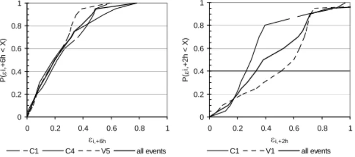
It is noticeable that the FR(τ) curve for all events tends towards the lower FR values associated with event V1. In this context it is of interest to examine the underlying CDF of εi,τ in detail. In Figure 7 the
distribution of the individual events are compared against the CDF of the joint sample of εi,τ for a
spe-cific lead time in each basin.
In case of the Besòs (Fig. 7 on the right) at the upper and lower bounds the CDF(τ =+2 h) for the events C1 and V1 are very close. However, there are clear differences concerning the shape and in rela-tion to the median of the distriburela-tions. These differ-ences are reflected in the CDF for all events. At first, for quantiles smaller than 0.2, the joint CDF follows the error distribution of event C1. Following, there is a transition area towards the CDF of event V1,
which is then approximated in the range of the quan-tiles 0.8 to 1.0. Apparently the distribution of the joint sample of εi,τ is determined by the prediction
errors of event C1 in the lower part and by the pre-diction errors of event V1 in the upper range. Ac-cordingly, the evaluation of the εi,τ at the 0.85
quan-tile is dominated by the prediction errors of event V1.
For the Traisen basin (Fig. 7 on the left) the CDF(τ = +6 h) for the joint sample of εi,τ and the
indi-vidual events are more homogeneous. The curves diverge for quantiles above the 0.6 quantile. Still, the joint CDF at the 0.85 quantile is well centered in relation to the individual distributions. Similar re-sults (not presented here) have been found for CDF corresponding to other lead times.
0 0.2 0.4 0.6 0.8 1 0 0.2 0.4 0.6 0.8 1 εi,+6h P( ε i, + 6h < X ) C1 C4 V5 all events 0 0.2 0.4 0.6 0.8 1 0 0.2 0.4 0.6 0.8 1 εi,+2h P( ε i, + 2 h < X ) C1 V1 all events 0 0.2 0.4 0.6 0.8 1 0 0.2 0.4 0.6 0.8 1 εi,+6h P( ε i, + 6h < X ) C1 C4 V5 all events 0 0.2 0.4 0.6 0.8 1 0 0.2 0.4 0.6 0.8 1 εi,+2h P( ε i, + 2 h < X ) C1 V1 all events
Figure 7. CDF of εi,τ for individual events compared to CDF of
εi,τ for all events: on the left the CDF(τ = +6h) in the Traisen
ba-sin; on the right the CDF(τ = +2h) in the Besòs basin.
Imlications of QPF uncertainty
The influence of ensemble QPF on the evaluation of FR is studied by a comparison with the results ob-tained when the deterministic QPF is used for flood forecasting. In Figure 8 the FR(τ) curves correspond-ing to an evaluation of the εi,τ samples based on
de-terministic QPF and ensemble QPF are shown. Overall the development of both curves is very similar. For lead times τ < +10 h no difference can be observed between the graphs. In this context it has to be kept in mind that according to the underly-ing procedure of QPF ensemble generation the spread of the ensemble develops progressively with lead time. For lead times τ < +2 h all ensemble members are identical.
Beyond τ > +10 h FR is reduced when QPF re-lated uncertainty is taken into account in terms of the ensemble QPF. Otherwise FR tends to be slightly overestimated.
Apparently, the prediction errors resulting from the ensemble QPF are at large very similarly distrib-uted as the error sample obtained by the use of the deterministic QPF (CDF not shown). Within the context of this study the reliability of the flood fore-cast does not seem to be improved by the use of the ensemble QPF. These findings are consistent also for the separated analysis of the individual events considered. FR (τ) 0 0.25 0.5 0.75 1 1 13 25 37 τ [h] FR (0 .85) QPFdet QPFens
Figure 8.Forecast reliability as a function of lead time τ in the
Traisen basin using either deterministic QPF or ensemble QPF
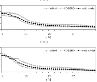
Implications of hydrological model uncertainty As discussed above, FR is related to the basic capa-bility of the hydrological model to reproduce the dy-namics of a specific flood event. The application of multiple hydrological models allows for a glimpse on the dependence of FR(τ) on the hydrological simulation model used. In Figure 9 the FR(τ) curve is broken down with respect to the models COSERO and WBrM.
The graphs for the evaluation of FR based on all events (Fig. 9 above) shows a systematic deviation between the models. These findings correspond to the differences in the basic model performance in terms of the Nash-Sutcliffe-Efficiency (cf. Table 1). This indicates that the evaluation of FR is condi-tioned by the capability of the simulation model to reproduce the dynamic behavior of the hydrological system.
However, the diagram in Figure 9 below, which shows FR(τ) for the event C4 using different models does not confirm this relation. For τ = +1 h WBrM provides more reliable predictions than COSERO. Then with increasing τ both curves intersect at τ = +4 h and the relation is reversed. This example dem-onstrates that the modulation of QPF input informa-tion depends on the hydrological model. So, it seems that there is a complex interaction between QPF in-put data and other factors included in the simulation model.
FR (τ) 0 0.25 0.5 0.75 1 1 13 25 37 τ [h] FR (0 .8 5 )
WBrM COSERO multi model
FR (τ) 0 0.25 0.5 0.75 1 1 13 25 37 τ [h] FR (0 .85)
WBrM COSERO multi model
FR (τ) 0 0.25 0.5 0.75 1 1 13 25 37 τ [h] FR (0 .8 5 )
WBrM COSERO multi model
FR (τ) 0 0.25 0.5 0.75 1 1 13 25 37 τ [h] FR (0 .85)
WBrM COSERO multi model
Figure 9. Forecast reliability as a function of lead time τ in the
Traisen basin using different hydrological models. Above: FR evaluation based on all events. Below: FR evaluation based on the event C4
5.1 Discussion
The results of the analysis show that the decrease of FR with increasing lead time can be principally at-tributed to the capability of the QPF method to an-ticipate future rainfall. However, the basic level of FR is determined by the performance of the hydro-logical model to reproduce the dynamic behavior of the hydrological system. In this respect, the re-sponses of multiple hydrological models add com-plementary information to the forecasting process. The relative importance of the hydrological model performance for the reliability of the flood forecasts decreases in contrast to QPF related uncertainty as lead time is extended.
As can be seen from the results for the Traisen basin, the model related level of FR is constant for lead times of approx. τ = +4 h. For this forecast ho-rizon, the information coming from rainfall observa-tions seems to persist. Beyond this point, the impor-tance of comparatively uncertain rainfall forecasts increases continuously with lead time and deterio-rates FR.
The results for the Besòs illustrate that input in-formation based on QPE is useful for the prediction of floods at best for a forecast horizon of τ = +2 h.
The lead time of approx. 4 – 6 h in the Traisen and approx. 2 h in the Besòs are within the range of the response time in each basin.
In comparison to these strong implications the ef-fect of explicitly quantified QPF related uncertainty in terms of ensemble QPF is of secondary order. However, the analysis of prediction errors integrates the forecasts of all ensemble members in a joint dis-tribution, thus obscuring the predictive performance of individual ensemble members.
Furthermore, it has been shown that FR is de-pendent on individual events (cf. Fig. 6). As can be observed from the results in the Besòs, which are de-rived on the basis of relatively small sample sizes of the prediction error, the evaluation of FR is highly influenced by the distributions’ shapes and the ranges of prediction errors of the particular events. Certainly, for a general interpretation of the results, it is necessary to include more events in the analysis. In view of these findings, it is problematic to de-termine whether or not the EWS are effective. Both EWS considered have demonstrated the potential to produce flood forecasts with an adequate level of re-liability.
The question whether these forecasts are avail-able with sufficient lead time requires taking a look at the preventive measures to be completed. Also, it has to be taken into consideration that the decision about a flood alert is very complex, involving a trade-off between numerous aspects. Therefore, the reliability of the flood forecast has to be assessed in the context of the potential damages and the conse-quences of an alert. In this regard, the FR(τ) curves presented have to be combined with a benefit func-tion that quantifies the (socio-) economic conse-quences of a decision by stating the potential dam-ages to be avoided and the damdam-ages a false alert might cause due to unnecessary precautionary meas-ures.
From the combination of the forecast reliability curve and the benefit function a warning expectation curve can be derived, which provides improved in-formation for the warning and allows for the identi-fication of the optimum point of time for triggering the alert.
6 CONCLUSIONS
A methodology has been proposed to evaluate the reliability of flood forecasts for early warnings as a function of lead time. Forecast reliability is quanti-fied on the basis of a straightforward interpretation of the cumulative distribution function of a sample of prediction errors. The prediction errors are ob-tained from the comparison of predicted discharges with available observations of past flood events.
The procedure has been applied in the context of two operational early warning systems. Within this framework the lead time dependence of flood fore-cast reliability has been determined. Further, the im-plications and the relevance of QPF related uncer-tainty and hydrological model unceruncer-tainty have been studied.
The results indicate that the hydrological model used to produce the flood forecast conditions the ba-sic level of forecast reliability. In this regard, it has been shown that the application of multiple models
is beneficial in order to include complementary in-formation in the flood forecast.
The anticipation of future rainfall is the decisive source of information for flood forecasts with lead times beyond the response time of the basin. Im-proving QPF and constraining the related uncer-tainty seems to be a key challenge for progress in flood forecasting. In this context, a differentiated analysis of the variation of forecast reliability asso-ciated with the individual ensemble members is of interest.
In consideration of the limited number of events analyzed within this explorative study, it is difficult to draw general conclusions concerning the effec-tiveness of the early warning systems. In particular, this is because forecast reliability turned out to de-pend on the different events and, in the case of the Besòs, is affected by the small sample size of the prediction errors.
Notwithstanding, the FR(τ) diagrams presented embrace the uncertainty associated with the flood forecast in relative terms. Hence, they provide a pos-sibility to include this information in the decision about an alert. For the evaluation of EWS efficiency this information is essential. These aspects are dis-cussed in detail in the companion paper (Gocht et al. 2008).
7 REFERENCES
Anquetin, S., Creutin, D., Delrieu, G., Ducrocq, F., Gaume, E.& Ruin, I. 2004.Increasing the forecasting lead-time of weather driven flash-floods. Research report No. H01/812/02/D9056/AG/ct. Laboratoire d'étude des trans-ferts en hydrologie et environnement. Grenoble. France. Berenguer, M., Corral, C., Sanchez-Diezma,
R.&Sempere-Torres, D. 2005.Hydrological valida-tion of a radar-based
nowcasting technique. Journal of Hydrometeorology.
6(4):532-549.
Bergstrom, S. 1992.The HBV model - its structure and applica-tions. SMHI reports, Norrköping. Sweden.
Bergstrom, S. 1995.The HBV Model. In V.P. Singh (ed.), Computer models of watershed hydrolog. Water Resources Publications.
Beven, K.& Kirkby, M. J. 1979.A physically based, variable
contributing area model of basin hydrology. Hydrological
Sciences - Bulletin - des Sciences Hydrologiques. 24(1):43-69.
Bowler, N. E., Pierce, C. E.& Seed, A. W. 2006.STEPS: A probabilistic precipitation forecasting scheme which merges an extrapolation nowcast with downscaled NWP. Quarterly Journal of the Royal Meteorological Society 132(620):2127-2155.
Buizza, R., Miller, M.& Palmer, T. N. 1999.Stochastic repre-sentation of model uncertain-ties in the ECMWF Ensemble
Prediction System. Quarterly Journal of the Royal
Mete-orological Society 125(560):2887-2908.
Clemen, R. T. 1989.Combining Forecasts - a Review and
An-notated-Bibliography. International Journal of Forecasting
5(4):559-583.
Collier, C. G. 2007.Flash flood forecasting: What are the limits
of predictability? Quarterly Journal of the Royal
Meteoro-logical Society 133(622):3-23.
Georgakakos, K. P., Seo, D. J., Gupta, H., Schaake, J.&Butts, M. B. 2004. Towards the characterization of streamflow simulation uncertainty through multi-model ensembles Journal of Hydrology 298(1-4):222-241.
Gocht, M., Schröter, K., Nachtnebel, H.P., Ostrowski, M. 2008. EWASE - Early Warning Systems Efficiency Risk
Assessment and Efficiency Analysis. Proceedings of the
European Conference on Flood Risk Management - Re-search into Practice. Oxford.
Haiden, T., Kann, A., Stadlbacher, K., Steinheimer, M.&Wittmann, C. 2007. Integrated Nowcasting through Comprehensive Analysis (INCA) - System overview. ZAMG report. Vienna. Austria.
Komma, J., Reszler, C., Blöschl, G. & Haiden, T. 2007. En-semble predictions of floods - catchment non-linearity and
forecast probabilities. Natural Hazards and Earth System
Sciences 7: 431-444.
Krzysztofowicz, R. 1999. Bayesian theory of probabilistic
forecasting via deterministic hydrologic model. Water
Re-sources Research 35(9):2739-2750.
Krzysztofowicz, R. 2001. Integrator of uncertainties for prob-abilistic river stage forecasting: precipitation-dependent
model. Journal of Hydrology 249(1-4):69-85.
Krzysztofowicz, R. & Maranzano, C. J. 2004. Hydrologic un-certainty processor for probabilistic stage transition
fore-casting. Journal of Hydrology 293(1-4):57-73
Lorenz, E. N. 1963.Deterministic Nonperiodic Flow. Journal
of the Atmospheric Sciences 20(2):130-141.
Mockus, V. 1957.Use of storm and watershed characteristics in synthetic hydrograph analysis and applications. Soil-Conservation-Service. U.S. Dept. of Agriclture.
Nachtnebel, H. P. & Kahl, B. 2007.Hochwasserprognosesystem Traisen – Hydrologische Abflussmodellierung. Amt der Nieder Österreichischen Landesregierung.
Nash, J. E. & Sutcliffe, J. V. 1970. River Flow Forecasting Through Conceptual Models Part I - Discussion of
princi-ples. Journal of Hydrology 10(282-290.
Ostrowski, M. 1991. The Effect of Data Accuracy on the
Re-sults of Soil Moisture Modeling. IAHS Publication.204.
Refsgaard, J. C., van der Sluijs, J. P., Brown, J. & van der Keur, P. 2006. A framework for dealing with uncertainty
due to model structure error. Advances in Water Resources
29(11):1586-1597.
Shamseldin, A. Y., Oconnor, K. M.&Liang, G. C. 1997. Meth-ods for combining the outputs of different rainfall-runoff
models. Journal of. Hydrology 197(1-4):203-229.
Todini, E. 2007. Hydrological catchment modelling: past,
pre-sent and future. Hydrology and Earth System Sciences
11(3):468-482.
Wang, Y., Haiden, T. & Kann, A. 2006. The operational lim-ited area modelling system at ZAMG:
ALADIN-AUSTRIA. Beiträge zur Meteorologie und
Geo-physik.37(33).
Wilson, J. W., Crook, N. A., Mueller, C. K., Sun, J. Z. & Dixon, M. 1998.Nowcasting thunderstorms: A status
re-port. Bulletin of the American Meteorological Society
79(10):2079-2099.
WMO 1992.Simulated Real-Time Intercomparison of Hydrol-gical Models. World MeteoroloHydrol-gical Organisation. Opera-tional Hydrology Report No. 779. Geneva.
Yates, D., Warner, T. T., Brandes, E. A., Leavesley, G. H., Sun, J. Z. & Mueller, C. K. 2001. Evaluation of flash-flood discharge forecasts in complex terrain using precipittion. Journal of Hydrologic Engineering 6(4):265-274.
Yates, D. N., Warner, T. T. & Leavesley, G. H. 2000. Predic-tion of a flash flood in complex terrain. Part II: A compari-son of flood discharge simulations using rainfall input from radar, a dynamic model, and an automated algorithmic