The effects of marginal employment on subsequent labour market outcomes

(1)

The effects of marginal employment on subsequent labour market outcomes von René Böheim und Andrea Weber*) Arbeitspapier Nr. 0612 Juli 2006

Johannes Kepler Universität Linz Institut für Volkswirtschaftslehre Altenberger Straße 69 A-4040 Linz - Auhof, Austria www.economics.uni-linz.ac.at *)

I

N

S

T

I

T

U

T

F

Ü

R

V

O

L

K

S

W

I

R

T

S

C

H

A

F

T

S

L

E

H

R

E

J

OOHHAANNNNEESS

K

EEPPLLEERR

U

NNIIVVEERRSSIITTÄÄTT

L

IINNZZ

(2)

The effects of marginal employment on

subsequent labour market outcomes

∗

Ren´

e B¨

oheim

Johannes Kepler University Linz and IZA, Bonn

Andrea Weber

†

UC Berkeley, Institute for Advanced Studies, Vienna, and IZA, Bonn

July 25, 2006

∗_{We thank Martina Zweim¨}_{uller for excellent research assistance. Many thanks to David} Card, Peter Huber, and Rudolf Winter-Ebmer for valuable comments and suggestions. This research was supported by the Austrian National Bank, Grant Nr 11090. Part of this research was conducted while Ren´e B¨oheim was at UC Berkeley, supported by the Austria-Berkeley Exchange Programme of the European Recovery Programme (‘Marshall Fund’). Andrea Weber gratefully acknowledges financial support form the Austrian Science Foundation, Project Nr J2365-G05 and from the Center for Labour Economics at UC, Berkeley.

(3)

The effects of marginal employment on subsequent labour

market outcomes

Abstract

We analyse the consequences of starting a wage subsidised job, “marginal employment”, for unemployed workers. Marginal employment is a type of wage subsidy paid to unemployed workers and they do not lose their un-employment benefits if the wage is below a certain threshold. We ask if the unemployed who start marginal jobs face better labour market out-comes than those who do not work. A priori it is not clear if those who work in marginal employment improve their labour market status, e.g. by signalling effort, or worsen it by reduced job search effort. We select unem-ployed workers and investigate the effect of marginal employment on their labour market outcomes, by means of propensity score matching. Our results suggest that selection into marginal employment is “negative”, i.e. workers with characteristics we usually associate with low-productivity are more likely to select into such jobs. The unemployed who start to work in marginal employment during their unemployment spell suffer a (causal) penalty for doing so, relative to their peers who do not. The penalty, in terms of less employment, more unemployment, lower wages, lessens over time but is still present after three years.

Keywords: marginal employment, atypical employment, labour supply, propen-sity score matching

(4)

1

Introduction

The causes for the high unemployment rates in (Western) Europe are highly de-bated, among the candidates are high wage levels which reduce the demand for workers, especially those with low levels of productivity; strict employment con-tracts and protection laws, which may not allow employers to react flexibly to short-term demand fluctuations; benefit systems, which are seen to provide lit-tle incentive for unemployed workers to find employment.1 _{Consequently, many}

labour market reforms focus on employment contracts that allow for more em-ployment flexibility (e.g. the recent attempt in France to extend the probationary period of youth workers) or incentive schemes to induce unemployed workers back into employment (e.g. the German Kombilohn).

In Austria, a special employment contract exists, “marginal employment”, which combines flexibility and incentives. Marginal employment (ME) is defined by wage income being below a threshold. In 2006, the threshold wase333.16 per month before tax, or about 19% of the median gross wage. Marginal employ-ment is an attractive type of contract for employers, because for these jobs social security contributions are substantially reduced and only minimal employment protection applies. It is attractive to the unemployed, because an unemployed worker does not lose any benefit entitlements while working in ME. In other words, ME provides a wage subsidy paid to the worker (Katz, 1998; Phelps, 1994). This wage subsidy has, for the unemployed claiming unemployment ben-efits, a discontinuity at the threshold, because benefits are fully withdrawn for any wage income above the ME threshold.

(5)

We analyse the marginal employment of unemployed workers and examine whether it facilitates their return to regular employment or not. Potentially, a marginal job may allow the worker to stay attached to the labour market and to signal motivation to employers. This way it would act as a “stepping stone” (Booth, Francesconi and Frank,2002). Alternatively, marginal employment could ultimately force workers out of the regular labour market, offering merely a “dead end” (Booth et al., 2002).

To evaluate the outcomes of marginal employment, we analyse new entrants into unemployment using data from the administrative registers. These data have the advantage of detailing, for each employee, the complete history of labour market spells. In the sample, we find that upon entry into unemployment many choose to become marginally employed before they start regular employment. Marginal employment is thus for many unemployed an option, but how does it effect their future careers?

We compare the unemployed who start marginal employment before return-ing to regular employment with those who do not. The data offer a wide range of outcome measures, we compare the days employed, the days unemployed, and the wages of the two types of the unemployed for up to three years after the start of their unemployment spell. The decision to become marginally em-ployed is most likely correlated with expected future labour market outcomes and marginally employed workers are then not a random sample of all unem-ployed workers. Since we have no source of exogenous variation in the entry to marginal employment, which would allow to model the selection into ME, we use propensity score matching to control for selection on observable characteristics

(Dehejia and Whaba, 1999; Rosenbaum and Rubin, 1984). The data provide a

(6)

previous experiences with marginal employment for an appropriate estimation of the propensity score.

There have been a number of studies examining the effect of temporary job placement on subsequent labour market outcomes over the last years. (Ichino, Mealli and Nannicini(2006) provide an overview.) Autor and Houseman (2005), using US data, find a negative association between between temporary jobs and subsequent labour market careers and argue that their finding is more robust than European studies because they exploit a semi-experimental setting. The European studies typically use some sort of matching technique and generally find a positive association between temporary jobs and subsequent labour market careers.

Our results show that marginal employment is, despite its popularity among the unemployed, associated with less employment, lower wages, and with more unemployment in subsequent periods. Although the negative effect of ME lessens over time, after three years these workers still fare worse than their peers. A way to improve chances of marginal workers in the labour market and facilitate transitions to regular employment might be to combine marginal employment with a more generous wage subsidy or incentive scheme in the context of active labour market policies, like suggested by Fertig, Kluve and Schmidt(2006).

2

Institutional Background

In Austria, health, pension, and unemployment insurance is compulsory for ev-ery employee. Social security contributions are split between the employer and the employee and amount in total to 39.9% of the gross wage. This makes

(7)

Aus-trian non-wage labour costs relatively high (see, for example, U.S. Department of Labor, 2005, Table 15).

Marginal employment is a special type of contract defined by wage income being below a certain limit. In 2006, the monthly limit for ME was e333.16, or about 19% of the median gross wage. Workers who are marginally employed are, by and large, exempt from compulsory social security. For them, the employer has to contribute 1.4% of the gross wage towards the employees’ insurance against work-related accidents. A marginally employed worker may voluntarily enroll into health and pension insurance by paying e46 per month, or 14% of the threshold for ME. Marginal jobs are not covered by the unemployment insurance system. Marginal workers are entitled to their (state) pension payments, or to unemployment benefits (and unemployment assistance), if eligible.

In Austria, unemployment benefits (UB) amount to 55% of previous net wages, plus a family allowance. The eligibility period is 20 or 30 weeks, depending on previous work experience. After exhaustion of UB, the unemployed worker can apply for unemployment assistance (UA), which is means tested. In case of continued eligibility, unemployment assistance can be claimed indefinitely. Re-cipients of unemployment benefits or unemployment assistance are fully covered by the state health insurance system and the time claiming UB counts towards state pension eligibility.

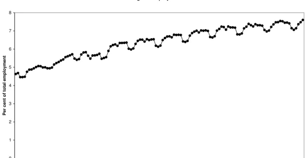
The importance of marginal employment in Austria has increased over the past years. Figure 1 plots the number of ME as a percentage of all employment from May 1995 to December 2005. Since 1995, employment in marginal jobs has increased from about 4.6 per cent of total employment to about 7.5 per cent in 2005. In a study about the sales sector in Austria Huber and Huemer (2004)

(8)

find a marked increase in marginal employment in retail sales after a relaxation of shop opening hours in 1997. The majority of marginal workers are women (70% in 2004). According toHuber and Huemer(2004), women also tend to stay longer in marginal employment and are less likely to switch to regular jobs than men.

3

Theoretical Considerations and Model

Marginal employment is a flexible, and cheap, instrument for employers to re-act to short-term demand fluctuations. The non-wage labour costs paid jointly by employer and employee are at least halved. In addition, flexible dismissal regulations apply as for marginal employment the period of notice is 14 days.

Marginal employment is attractive for two groups of workers. The first group are workers who are detached from the labour force, i.e. either not working in a regular job or out-of-the labour force. A marginal job may provide access to the social security system and thus relatively cheap access to pension and health insurance. The second group are unemployed workers, especially those who claim UB, because income from ME is added to the benefit income.2 _{We focus on the}

second group and investigate the effect of marginal employment started during an unemployment spell on the worker’s future wage and employment outcomes. We do not consider that ME may offer an entry to the labour market for persons who are out-of-the-labour force.

2_{A third group would be those who want to supply many hours of work, but are hours} constrained in their main job. However, multiple job holding is relatively uncommon in Austria. Only about 4% of regular workers hold a second job. Likewise, we find few workers in two or more marginal jobs.

(9)

Marginal employment has some features that make it comparable to a wage subsidy program. A wage subsidy is typically individually based, not means-tested, and has a limited duration. Where wage subsidies are provided to in-dividuals, rather than directly to firms, eligibility usually depends on a certain duration of unemployment insurance receipt. Usually the wage subsidy also im-poses a minimum working requirement. Marginal employment, on the other hand, allows the unemployed benefit recipient to earn extra income if they supply few hours, or earns a wage below the threshold. As soon as the threshold is crossed, however, UB is withdrawn completely. Consequently, the unemployed worker faces a discontinuous hours choice, which is sketched in Figure 2. The graph draws the relationship between earnings and hours worked for a given wage rate

w. An unemployed worker’s earnings equal the benefit levelb. By supplying a few hourshM E of work in a marginal job the worker earnsb+M E, benefits plus the

ME threshold. Jobs which put wage income slightly above the marginal threshold are unattractive, because they generate less income than income from benefits alone. In order to be strictly better off the worker would have to supply as many hours as to receive earnings above the benefit level plus the marginal threshold, in the graph this is hE. The gap between hM E and hE, or the magnitude of

the discontinuity, depends on the benefit levelb. Consequently, the discontinuity may be especially important for full-time workers, as the benefit level depends on earnings in the previous job.

What are the behavioural responses that we expect from unemployed workers? Because of the discontinuity in hours choices we expect workers to start a marginal job and to collect benefits for a prolonged time, or to start a regular job relatively quickly. This means that the short-term effects of the marginal job are determined by the behavioural responses generated by the incentives on earnings and hours

(10)

choices. The causal effects of ME on future employment and wage outcomes will be revealed over a medium time horizon.3

Because there are no special restrictions to receiving the wage subsidy implicit in marginal employment other than benefit eligibility one may ask whether this system induces individuals to reduce their work effort in order to benefit from the subsidy. We think that the sharp discontinuity mitigates the negative incentives created by this system. In order to address the issue of windfall beneficiaries or collusions between firms and workers we investigate how take-up varies with the elapsed unemployment duration and whether employers rehire their former employees as marginal workers or not.

We choose the following setup for the empirical analysis. We sample work-ers entering unemployment and compare those taking up ME within the first 6 months of their unemployment spell with workers who do not enter ME before their unemployment spell ends. (We drop individuals entering ME after 6 months from the sample.) We call the first the ME group and the other the control group. The choice of 6 months appears somewhat arbitrary, but it corresponds to the average UB entitlement period (remember that the entitlement period is either 20 or 30 weeks depending on prior work experience.)

For these two groups, we compare wage and (regular) employment outcomes in the first, second, and third year after the start of unemployment.

To account for non-randomness in the choice to start ME we use a propensity score matching technique. The matching is valid, if conditional on all information available at the start of the unemployment spell starting ME is random. This

3_{We do not expect special effects to occur upon benefit exhaustion, because the Austrian} system with the combination of unemployment insurance and unemployment assistance allows basically for an unlimited benefit period.

(11)

further implies that at the beginning of the unemployment spell an individual, with given characteristics, faces a job finding rate that is known to him and which is constant over time.

One problem is that the matching approach assumes that the propensity to work ME is independent of elapsed unemployment duration. For example, if prospects for regular employment deteriorate over time, an unemployed worker may become more likely to accept a marginal job. By conditioning on charac-teristics at the start of the spell we cannot control for time-varying changes of behaviour. Our strategy to assess the importance of this problem is to check the robustness of our results by selecting different ME groups, based on varying lengths of elapsed unemployment duration (three, six, and twelve months). We also estimate the effects of ME for a smaller sample of workers who had no ME experience in the five years preceding the unemployment spell. We further exam-ine the robustness of our results by comparing them to those for the unemployed who were employed the whole month prior to the unemployment spell.

4

Data

We use data on individual labour market careers from Austrian administrative records. Our sample consists of the total inflow into unemployment between March and August 1999.4 _{To avoid conflicts with time spent in education, or}

(early) retirement, we only consider workers between 20 and 50 years of age. This leaves us with a sample of 193,276 unemployed. All our analyses are carried

4_{We define an individual as unemployed if she is either collecting unemployment benefits or} actively searching for work, but not working in regular employment. For those with multiple spells in this period, we select the first unemployment spell.

(12)

out separately for women (93,896) and men (99,380), because women are more likely to work in ME than men are.

We combine individual data from two different sources, (i) theAustrian social security database which contains detailed information on the individuals’ employ-ment, unemployment and earnings history, and information on the employer (e.g. region and industry); and (ii) the Austrian unemployment register from which we get socio-economic characteristics. We use information on employment and wage histories for the period 1993 to 2001, i.e. five years before and three years after the start of the spell. The records contain, for each day, information on the labour market status and we distinguish between regular employment, marginal employment, unemployment, parental leave, and non-participation.

The median unemployment duration in the sample is 1.8 months (mean is 4 months) and 6% of the individuals are unemployed longer than 12 months. Unemployment spells end in most cases (80%) because of the start of a regular employment spell, the remaining unemployment spells end because of withdrawal from the labour market (maternity, retirement, or other, unknown, reasons.)

Upon entry into unemployment, history and outcomes are measured in one-year intervals from that date. While the data are appropriate for our research as they provide precise labour market histories for a long period, they also have limitations. The most restricting for our application is that the data do not detail the hours of work and we therefore cannot identify part-time work.5 _{Wages are}

measured as the average of monthly wages over all regular jobs during the year, and are deflated to 2005 prices (in Euros). No wages are available for marginal

5_{The share of part-time work in all employment in 1999 was 16.4%: 32.4% of women and} 4.4% of men worked in part-time jobs in 1999 (Statistics Austria, 2006).

(13)

jobs and the wage is set equal to zero for individuals with no regular employment during the year.

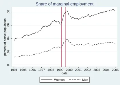
In Figure3, we plot for our sample of unemployed workers the monthly share of marginal workers, from 1994 to 2004. It is apparent that the share of ME increases sharply upon entry into unemployment. The inflow period into un-employment 03-08/1999 is marked by vertical lines. During that time marginal employment increases by about two percentage points for women and by about one percentage point for men. Over the following six months the shares of ME re-vert to the trend. This suggests that on becoming unemployed workers are more likely to start a marginal job. The figure also confirms the high share of women in marginal employment noted by Huber and Huemer(2004). The trend in our sample resembles the trend of marginal employment for the whole population, plotted in Figure 1.

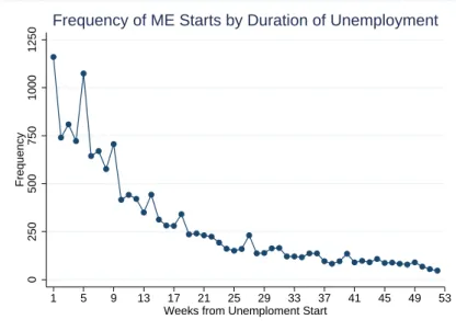
Figure 4shows the frequency of ME starts by the elapsed unemployment du-ration. We see that the majority of ME spells start a short time after entry into unemployment, most of the marginal spells start within 2 months form unem-ployment entry. Usually it requires some time to search for a (marginal) job and the picture confirms that we capture most of the workers who start ME within 6 months upon entry to unemployment.

Table 1 presents the incidence of marginal employment in our sample and describes the composition of ME and control groups our analysis is based on. The control group consisting of individuals who never take up a marginal job before returning to regular employment, or before their unemployment spell ends is 178,427 individuals (84,105 women). We have 11,965 individuals taking a marginal job within 6 months of becoming unemployed. The share of marginal

(14)

workers among women (8.5%) is twice as high as among men (4.2%). If we restrict the ME group to individuals taking up ME within the first three months of unemployment the share of marginal workers in the full sample (consisting of ME and control group) is reduced to 4.7% on average, whereas it is 7.7% if we allow for all individuals taking a marginal job during the first year.

As a separate robustness check we will restrict the sample to individuals who were employed for at least one day in the month before entering unemployment. This reduces the sample by about 25%, the share of marginal workers remains the same though.

To address the potential problem of windfall beneficiaries or collusion between employers and employees who agree to substitute regular employment for UB plus ME, Table 2 presents recall rates to the same employer among the various employment states. The overall recall rate in the Austrian economy, i.e. those who work for the same employer before and after the unemployment spell, is relatively high (Pichelmann and Riedel, 1992), in our sample the recall rate is some 33 per cent for women and about 22 per cent for men. The recall rate from a marginal job to regular employment, for individuals finding a job after unemployment, is 27% and about as high as the overall rate. It occurs much less often that an employer lays off an individual from a regular job and rehires them as marginal worker. The recall rate from a regular job to a marginal job is only 15%. This means that the number of windfall beneficiaries generated by ME cannot be particularly high, as we expected.

In the Appendix, Table A-1, we present descriptive statistics, separately for the ME and the control group. If we consider age, educational attainment or marital status, we see little differences between women who started ME and

(15)

those who did not. When we consider past labour market experiences, we find that more of those who started ME have had previously worked in ME than those in the control group, suggesting that some persistence is present in those who work ME. In the year before the start of the unemployment spell, women who started ME had worked on average some 82 days in ME. This contrasts with an average of some 20 days for those who did not start ME. Those who started ME have had fewer employment spells in the year preceding the unemployment spell (women, 1.2, and men, 1.5) than those who did not (women, 1.5, and men, 1.7). The difference between the two groups in terms of days employed is about two weeks for women and about one week for men, with those who did not start ME having worked more days. On average, those who did not start ME had higher wages (women: e966 vs. e811; men: e1,418 vs. e1,273).

Those who started ME have had, two years earlier, consistently fewer days in regular employment, they had earned lower wages, and they have had more days in ME than those in the control group. The farther we go back in time, however, the smaller the differences between the two groups become.

Looking at the descriptive statistics of the outcome variables, we observe that those who chose ME had spent, on average, fewer days in (regular) employment, spent more days in unemployment, and earned a lower wage than those in the control group. Over time, the differences become smaller, but they do persist. In the third year after the start of the unemployment spell, apart from the men-tioned differences in wages, hardly any differences remain for women; for example, average days employed were 216 (control) and 213 (ME) days. Differences are greater for men. Men who chose ME spent about three weeks less in employment than those who did not choose ME, their wages were about 10% lower, and their average unemployment duration was about a week longer.

(16)

5

Method

Our aim is to estimate the average effect of marginal employment (ME) on labour market outcomes for those unemployed who start ME before they enter regular employment. In order to estimate the “average treatment effect on the treated” (ATT), we would like to compare labour market outcomes for unemployed workers who started ME with the counterfactual outcome in case they did not start ME. Since we never observe both outcomes for the same individual, we need to com-pare observations on individuals entering marginal employment (ME group) with observations on individuals who do not (the control group). A direct comparison of average outcomes of these two groups of unemployed may be confounding the true effect, because an individual’s decision to start ME is most likely related to expected future labour market outcomes. For example, imagine that highly skilled workers are less likely to start ME than those with few skills. As a con-sequence of the different skill compositions in the ME and the control group, we may observe differences in mean wage outcomes in both groups, which are not driven by ME, but by differences in productivity.

In order to control for such factors confounding the true effect of ME, our strategy is to compare the outcomes for individuals who are as similar as possible in terms of their predetermined characteristics. The main assumption is that selection into ME is based on observable characteristics and conditional on this information the individual’s decision to start ME is random.

To be more specific, let Yi1 be individual i’s outcome variable if she enters ME, and Yi0 the counterfactual. Further, let T1 be an indicator variable equal 1

(17)

if the individual decides to enter ME, and 0 if she does not. The ATT, or the average effect ME has on those who start ME, can be expressed as

AT T =E(Yi1|Ti = 1)−E(Yi0|Ti = 1).

As mentioned before, this expression cannot be estimated directly, because Yi0 is not observed for ME individuals. Assuming selection on observable covariates

Xi, namely Yi1, Yi1 ⊥Ti|Xi, we obtain

E(Yij|Xi, Ti = 1) =E(Yij|Xi, Ti = 0) =E(Yi|Xi, Ti =j)

forj = 0,1. In other words, the assumption means that conditional on observable variables Xi there is no systematic difference between the ME group and the

control group at the point of entry into unemployment. It allows us to identify the average treatment effect on the treated in the following way:

AT T =E[E(Yi|Xi, Ti = 1)−E(Yi|Xi, Ti = 0)|Ti = 1].

A nonparametric estimate may still be difficult to obtain, if X has many di-mensions and it would amount to finding a perfect counterpart for every ME individual in the control group. Rosenbaum and Rubin (1984) have shown that the information in Xi can be summarised in a single variable, the propensity

scorep(Xi). The propensity score is the conditional probability that individual i

with observable covariatesXi is taking up ME,

(18)

Therefore, instead of comparing individuals with identical X’s, it is sufficient to compare individuals with similar values of the propensity score and estimate the ATT by

AT T =E[E(Yi|p(Xi), Ti = 1)−E(Yi|p(Xi), Ti = 0)|Ti = 1].

The empirical estimation proceeds in two steps. First, we estimate the propensity score, separately for women and men. Conditional on the propensity score each individual has the same probability of taking a marginal job, as in a randomised experiment. We use this proposition to assess our estimates of the propensity score and group observations into blocks with similar values of the estimated propensity score to check whether the distributions of the observed covariates for ME and controls coincide in each group or not (“balancing” the distributions). The estimation of the propensity score is augmented by interaction terms and polynomials of variables in X until we succeed in balancing the covariates in each block.

In a second step, given the estimated propensity score from the balanced dis-tribution, we estimate a univariate nonparametric regressionE(Yi|p(Xi), Ti =j)

for j = 0,1. We use two different matching methods to construct the con-trol group, nearest neighbour matching and stratification matching. The nearest neighbour method searches for each ME observation an observation in the control group with the closest value of the propensity score. Subsequently the average outcomes in the ME and matched control samples are compared. The strati-fication method sorts observations from the lowest to the highest value of the propensity score. Then strata, defined on the estimated propensity score, are chosen such that the distributions of covariates is balanced between ME and

(19)

controls. We use the groups on which we based the balancing of the propensity score. Within each block we take the mean difference in outcomes between ME observations and controls, and weight these by the number of ME observations in each block.6

6

Results

6.1

Propensity Scores

We estimate the propensity score with a logit model of the propensity to start ME, using a range of the workers’ characteristics, including the labour market history up to five years in the past. In addition, we include interaction terms and polynomials in order to balance the distributions of explanatory variables between the control and ME groups. The estimation results are tabulated in the Appendix, TableA-2, and significance tests are given in Table A-3.

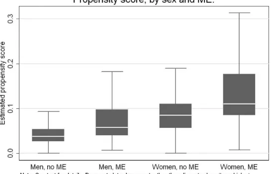
Figure 5shows box plots of the distributions of propensity scores for the ME and the control groups, for men and women. These plots provide a check of the comparability of the ME and the control group in terms of observable character-istics.7 _{A wider overlap in the distributions of the propensity scores results in}

better matches between observations in the treatment group and observations in the control group. The box plots show that the propensity scores are lower than

6_{We use Stata and the routines by} _{Becker and Ichino}₍₂₀₀₂_).

7_{The box plots depict for each of the four groups the distribution of the propensity scores.} The interquartile range, i.e. the distance between the 25th and the 75th percentile, is depicted by a (grey) box. The line within that gray box gives the median. The “whiskers” extend to the adjacent values, which separate the outliers from the rest of the data. The adjacent values are the 25th (or the 75th) percentiles minus (plus) 1.5 times the distance between the 25th and 75th percentiles (the interquartile range). For sake of clarity, we have excluded outliers from the graph; however, the outliers are used in our calculations. The maximum propensity scores are 0.669 for men, no ME; 0.714 for men, ME; 0.661 for women, no ME; 0.685, women, ME.

(20)

0.3 for women and lower than 0.2 for men for most of the observations in our data. While the control groups have typically lower values of the propensity score than those who started ME, the distributions do overlap and provide adequate support for the matching procedures.

Figures 6 and 7 plot the estimated propensity scores against labour market outcomes, the days employed, days unemployed, and wages in the first year after entry into unemployment. We group the estimated propensity scores into 40 blocks of equal size and calculate average outcomes for ME and controls in each block. The difference in outcomes in each block provides the ME effect at a constant value of the propensity score, i.e. holding observable characteristics fixed.

Figure 6 reveals that women with ME were employed for fewer days than women in the control group and that this difference is about the same size at all levels of the propensity score. The graph also shows a negative relationship between days employed and the propensity to work in ME for propensity scores of less than 0.12. At low values of the propensity score, women who have lower chances to be employed in a regular job are more likely to start ME than those with better chances. At higher values of the propensity score, the selection mech-anism seems to revert and women who face better employment outcomes are more likely to enter ME.

Remember that a worker who has a marginal job is still entitled to UB. This entitlement may explain the widening gap in the number of days unemployed as the propensity score increases because women who are more likely to enter ME are also collecting UB for a longer period than the control group. The relationship between wages in the first year after entering employment and the

(21)

estimated propensity scores is markedly negative for those with low propensity scores. Women around the median propensity level, around 0.085 for the control group and about 0.11 for the women with ME, earn monthly wages well below e1,000.

Figure7shows the corresponding graphs for male workers. The gaps between ME and controls are greater than for female workers, which suggests an even stronger negative effect of ME for men. Again we notice that the distribution of the propensity scores is more concentrated at low levels for men. There are only three bins for propensity scores higher than 0.1 and negative selection into ME is even more evident for men than for women.

6.2

Matching Estimates

Our estimation results of the average treatment effect on the treated (ATT) are presented in Table3. For each outcome variable, we estimate the ATT using the stratification method and the nearest neighbour method of matching. The choice of matching method matters little, the differences between the estimated ATTs are small. We discuss only the results from the stratification method.

For the outcomes in the first year since the start of the unemployment spell, we estimate that women who start ME spend about 40 days less in employment than the control group, which corresponds to about 30 per cent of the control group’s mean days employed. The ATT has a small standard error of 1.4. The results for men are similar, the difference in days employed is about 49 (SE of 1.8). This difference is about 33 per cent of the control group’s mean days employed. Considering the time spent in unemployment, women who work in ME spend some 30 days more in unemployment than those who do not, men are estimated

(22)

to spend some 40 days more in unemployment than those who do not work in ME.

The estimated ATT for the monthly wage in the first year states that women who started ME earn about e136 less per month than women in the control group. Men who started ME are estimated to earn e207 less per month than those in the control group. The estimated reduction in wages caused by ME amounts to about 15 per cent of the average monthly wage of women (e965) who are in the control group. Men in the control group earned on averagee1,390 and the reduction due to ME amounts to about 16 per cent. This large effect is most likely a combination of an employment and wage effect, because employment is considerably lower during the first year and wages of those who were not employed in the year are set equal to 0.

These “short-term” effects during the first year are well in line with our con-siderations about the behavioural incentives in section3. Especially, we find that individuals who take up ME are much longer unemployed, which is not surpris-ing given the possibility to claim UB while besurpris-ing marginally employed. On the other hand, those who move to regular employment directly have less incentive to exhaust their full benefit entitlement. In the second and third year after un-employment entry, the the possibilities to claim are much smaller, because of restricted access to prolonged benefits, making it less desirable to remain un-employed. We believe that the causal relationship between ME and subsequent labour market performance is revealed in the medium-term, i.e. once the UB’s incentives have worn out for the majority of the unemployed.

By looking at the outcome variables in the second year after the start of the unemployment spell, we see that the differences are indeed smaller. For example,

(23)

women with ME work about 6 days less than women in the control group; for men, the difference is some 10 days. When we look at days unemployed, we find no statistically significant difference between workers with and without ME. When we consider wages, we still estimate that those with ME earn less than those with no ME. For women it is about e76 less per month, or about 6 per cent of the control group’s average wage in the second year. For men, the difference is about e115 per month, or about 9 per cent of the control group’s average wage.

In the third year after the start of the unemployment spell, the differences between those with and those without ME are somewhat smaller than in the second year. However, we still estimate a negative effect of starting ME on labour market outcomes, be it days employed, days unemployed, or in terms of wages. Women who started ME are estimated to have slightly better outcomes in terms of days unemployed, they are estimated to spend about 4 days less in unemployment than those in the control group. Women with ME are estimated to spend about 2 days less in employment (these estimates are not statistically significant at conventional levels) and they earned e56, or about 6%, less per month than women in the control group. Men with ME spent about 9 days less in employment, about 4 days more in unemployment, and earned e90, or about 7%, less per month than men in the control group.

Overall we find negative effects of ME on all employment and wage outcomes. Throughout men are more effected by ME than women. The medium-term results point at small and negative employment effects of about one week. The wage effects are, however, still considerable after the third year. Because the differences in employment are relatively small, the difference in wages between ME and controls is arguably a pure wage loss effect.

(24)

The persistent wage penalty could arise from the fact that those who started ME have a preference for part-time work and those in the control group seek full-time employment. The difference in wages would thus be merely driven by the resulting difference in hours worked. While this is a possible critique of our results—remember that we do not know the number of hours worked—we do not consider it a likely explanation, because although the number of part-time workers has increased, especially for women, it is still almost negligible for men.

6.3

Robustness checks

Elapsed unemployment durationAs we discussed above, our estimation technique does not allow for the elapsed unemployment duration to affect the probability of starting ME. It is probable that some workers have an increasing risk of ME the longer they are unemployed, for others, this risk might be falling. We have re-estimated the ATTs for different durations of elapsed unemployment and starting ME.

Table 4 reports the results for the smaller group of individuals who started ME in the first 3 months after becoming unemployed, and for the group of all individuals who started ME during the first year after becoming unemployed. Comparing these results to the baseline case in Table 4, we see that the choice of the treatment group makes indeed a difference. All effects are smallest for the group of unemployed who start ME during the first 3 months and largest for the group who started in the first 12 months. For example, the employment effects are two days in the first case and -10 days in the second case for the third year for women, and -5 and -15 days for men. Wages per month in the third year are e38 or e83 lower for female ME workers and e66 or e133 lower for males,

(25)

depending on the length of the entry period. This result indicates that we cannot fully control for selection into ME by matching on the conditions at the start of the unemployment spell, because changes in behaviour over time seem to play a role. However, although the magnitude of the effects depends on the choice of the ME group, the main result is unchanged. Marginal employment has a negative, if small, impact on future employment and substantial negative wage effects in all samples.

Selection effects We have seen above that while most unemployed enter unem-ployment from a previous job, not all of them do so. ME is attractive, amongst other things, because it provides relatively cheap access to social insurance. Ar-guably some workers are less attached to the labour market, for example, those who start searching for a job without being entitled to UB, and have therefore different search strategies than workers who are closely attached to the labour market.

We re-estimated the ATTs of ME by restricting our sample to workers who en-ter unemployment directly from employment, rather than from any other labour market state. (Entry period to ME is six months.) The results from this exer-cise are tabulated in Panel 1 in Table5. We note that the results show a greater penalty from working ME in subsequent periods than the results presented above. The negative effects of ME lessen over time, but they are still present in the third year after the start of the unemployment spell.

In particular, focussing on the medium-term outcomes after three years, we estimate for women in this subset a wage penalty of about e60 per month, in comparison to their peers who did not start ME. For men, the wage penalty is about e126.

(26)

We noted above, that previous experience of ME makes a worker more likely to start ME, all other things equal. Again, we worry that the previous experience of ME, although we control for this in the estimation of the propensity score, might be associated with unobserved characteristics that are correlated with our outcome measures. We therefore restrict the sample to workers who had no experience of ME in the five years prior to the unemployment spell and estimate the ATTs of ME. The results are tabulated in Panel 2 of Table5. We see that for this subgroup of workers, the negative effects are slightly less severe for women and slightly more negative for men.

7

Summary and Conclusions

In our analysis, we investigated the consequences of starting a marginal job for unemployed workers. In particular, we asked ourselves whether the unemployed who work few hours face better labour market outcomes than those who do not work while collecting UB. A priori it is not clear if those who work in ME improve their labour market status, by signalling effort, possibly increasing the job offer arrival rate, etc., or worsen it by reducing their job search efforts.

Our results strongly indicate that for unemployed workers there is no positive consequence of marginal employment on subsequent regular employment. Our results are more in line with the US evidence inAutor and Houseman(2005) and stand in contrast to European studies, which find a positive effect of temporary jobs on transitions to regular employment. Marginal employment does not act as a stepping stone into regular jobs and all outcome measures we investigate— employment, unemployment, and wages—are less favourable for workers who

(27)

and more persistent over time for men than for women. Differences in outcomes lessen over time, for example, after three years, women who started ME earn about 6% less than women who did not. For men, neither employment nor wages of marginal workers catch up with workers in the control group after three years, wages are about 7% lower.

We also find that unemployed workers who are most likely to start marginal employment are individuals who are typically disadvantaged in the labour market, i.e. the young, those with little formal education, and those with interrupted employment careers. A worker with these characteristics would be the target of standard active labour market policy measures. Unemployed workers who are entitled to benefits are more likely to take a marginal job than those who have no entitlement.

A way to improve chances of marginally employed workers in the labour mar-ket would to integrate ME into the government’s active labour marmar-ket policy, where private sector employment programs already exist. ME is an income sub-sidy for workers who are eligible for UB and supply a minimum amount of hours. For jobs earning just above the marginal threshold, however, no subsidy is avail-able and the full social security contributions have to be paid. This creates a huge disincentive to work in these kind of (part-time) jobs above the marginal threshold.

An extension of the income subsidy towards jobs with higher wages could create incentives for labour supply in the jobs above the marginal threshold and possibly also facilitate transitions into regular jobs. The idea would be to allow unemployed workers to keep a share of their UB, which reduces with wage earned, in order to phase out the discontinuity created by the marginal threshold. At

(28)

the same time social security contributions could be reduced for these jobs to create an incentive for employers to hire more workers. Of course the subsidy has to be limited in time and restricted to special target groups, e.g long-term unemployed, in order to prevent windfall beneficiaries. For several countries positive experiences with income subsidy measures of this type exist, like the US, Canada, and the UK where they were part of the welfare reforms (Blundell and Hoynes, 2004;Card and Hyslop, 2005).

References

Autor, David and Susan N. Houseman (2005), ‘Do temporary help jobs improve labor market outcomes for low-skilled workers? Evidence from random assign-ments’, unpublished . Department of Economics, MIT.

Becker, Sascha O and Andrea Ichino (2002), ‘Estimation of average treatment effects based on propensity scores’, The Stata Journal 2, 358–377.

Blundell, Richard and Hillary Hoynes (2004), Has ’In-Work’ benefit reform helped the labour market, in D.Card, R.Blundell and R.Freeman, eds, ‘Seeking a Premier Economy: The Economic Effects of the British Economic Reforms, 1980-2000’, University of Chicago Press for NBER, Chicago, pp. 411–459. Booth, Alison, Marco Francesconi and Jeff Frank (2002), ‘Temporary jobs:

step-ping stones or dead ends’, The Economic Journal 112, F189–F213.

Card, David and Dean R Hyslop (2005), ‘Estimating the effects of a time-limited earnings supplement for welfare-leavers’, Econometrica 73, 1723–1770.

(29)

Dehejia, Rajeev H. and Sadek Whaba (1999), ‘Causal effects in nonexperimen-tal studies: Reevaluating the evaluation of training programs’, Journal of the American Statictical Association 94, 1053–1062.

Fertig, Michael, Jochen Kluve and Christoph Schmidt (2006), ‘Der erweiterte Minijob f¨ur Arbeitslose - ein Reformvorschlag’, Perspektiven der Wirtschaft-spolitik . forthcoming.

Huber, Peter and Ulrike Huemer (2004), ‘Besch¨aftigung im Handel - Vorl¨aufige Fassung’, WIFO Vienna, unpublished manuscript.

Ichino, Andrea, Fabrizia Mealli and Tommaso Nannicini (2006), ‘From tempo-rary help jobs to permanent employment: What can we learn from matching estimators and their sensitivity?’, IZA Discussion Papers(2149).

Katz, Larry (1998), Wage subsidies for the disadvantaged, in R.Freeman and P.Gottschalk, eds, ‘Generating jobs’, Russell Sage Foundation, New York, pp. 21–53.

Nickell, Stephen (1997), ‘Unemployment and labor market rigidities: Europe versus North America’, Journal of Economic Perspectives11(3), 55–74. Phelps, E S (1994), ‘Raising the employment and pay of the working poor: low

wage employment subsidies vs the welfare state’,AER Papers and Proceedings

pp. 54–58.

Pichelmann, Karl and Monika Riedel (1992), ‘New jobs or recalls? Flow dynamics in Austrian unemployment reconsidered’, 19, 259–274.

(30)

Rosenbaum, Paul R. and Donald B. Rubin (1984), ‘Reducing bias in observa-tional studies using subclassification on the propensity score’, Journal of the American Statictical Association 79, 516–524.

Statistics Austria (2006), ‘Statistical yearbook’. http://www.statistik.at/ jahrbuch_2006/englisch/start.shtml.

U.S. Department of Labor (2005), ‘Social insurance expenditures and other la-bor taxes as percent of hourly compensation costs for production workers in manufacturing, 32 countries or areas 1975-2004’, Bureau of Labor Statistics

(November). ftp://ftp.bls.gov/pub/special.requests/ForeignLabor/ ichccsuppt15.txt.

(31)

Figure 1: Marginal employment in Austria, per cent of total employment, May 1995–December 2005. Marginal Employment 0 1 2 3 4 5 6 7 8 05-95 09-95 01-96 05-96 09-96 01-97 05-97 09-97 01-98 05-98 09-98 01-99 05-99 09-99 01-00 05-00 09-00 01-01 05-01 09-01 01-02 05-02 09-02 01-03 05-03 09-03 01-04 05-04 09-04 01-05 05-05 09-05 Time P e r c e n t o f to ta l e m p lo y m e n t

(32)

Figure 2: Hours earnings relationship and hours choices under ME. b hours earnings w ME+b hME h_E

Figure 3: Development of marginal employment over time in the sample; vertical lines mark the inflow period into unemployment.

0

.02

.04

.06

.08

percent of active population

1994 1995 1996 1997 1998 1999 2000 2001 2002 2003 2004 2005 date

Women Men Share of marginal employment

(33)

Figure 4: Frequency of marginal employment starts by duration of the unem-ployment spell 0 250 500 750 1000 1250 Frequency 1 5 9 13 17 21 25 29 33 37 41 45 49 53 Weeks from Unemploment Start

(34)

(35)

Figure 6: Outcomes in the first year by propensity score, women. 50 100 150 200 250 days 0 .1 .2 .3 .4

Mean propensity score, in 40 bins Marg employment Control Women employment outcome first year

100 150 200 250 days 0 .1 .2 .3 .4

Mean propensity score, in 40 bins Marg employment Control

Women unemployment outcome first year

600 800 1000 1200 1400 Euro 0 .1 .2 .3 .4

Mean propensity score, in 40 bins Marg employment Control Women wage outcome first year

(36)

Figure 7: Outcomes in the first year by propensity score, men. 100 150 200 250 days 0 .1 .2 .3

Mean propensity score, in 40 bins Marg employment Control Men employment outcome first year

100 150 200 250 days 0 .1 .2 .3

Mean propensity score, in 40 bins Marg employment Control Men unemployment outcome first year

800 1000 1200 1400 1600 Euro 0 .1 .2 .3

Mean propensity score, in 40 bins Marg employment Control Men wage outcome first year

(37)

Table 1: Sample description

Females Males Total

Control Group 84,105 94,322 178,427 ME Group ME within 6 months 7,789 4,176 11,965 8.48% 4.24% 6.28% ME within 3 months 5,587 3,143 8,730 6.23% 3.22% 4.66% ME within 12 months 9,791 5,058 14,849 10.43% 5.09% 7.68%

Enter Unemployment from Employment*

Control Group 61,312 69,899 131,211

ME within 6 months 5,303 3,015 8,318

7.96% 4.14% 5.96%

Note: Control group - individuals who never take up a marginal job before their unemployment spell ends

ME group - individuals entering a marginal job while unemployed and within x months after unemployment start

percentages taken over the sum of ME and control group

(38)

Table 2: Recalls to the Same Employer

Females Males Total

Job to ME Recall Rate 16.07% 13.37% 15.09%

Number of Observations 8,318

ME to Job Recall Rate 27.24% 26.12% 26.83%

Job to Job Recall Rate 33.37% 21.95% 27.32%

Note: xxx

Table 3: Estimated average effect of Marginal Employment (ATT).

Women Men

Stratification Nearest Neighbour Stratification Nearest Neighbour

ATT (SE) ATT (SE) ATT (SE) ATT (SE)

The first year

Employment -40.762 (1.37) -39.936 (2.03) -48.866 (1.76) -51.164 (2.67)

Unemployment 30.523 (1.26) 30.478 (1.81) 37.647 (1.67) 40.388 (2.37)

Wage -138.637 (7.61) -135.885 (10.93) -207.508 (12.59) -227.148 (17.92)

The second year

Employment -5.564 (1.77) -3.979 (2.46) -9.927 (2.23) -12.646 (3.23)

Unemployment -2.133 (1.19) -1.827 (1.66) 1.935 (1.68) 3.543 (2.35)

Wage -76.047 (7.55) -69.317 (10.95) -115.155 (12.47) -130.973 (18.42)

The third year

Employment -2.032 (1.16) -2.807 (1.63) -8.798 (2.34) -10.699 (3.39)

Unemployment -3.937 (1.30) -5.101 (1.86) 3.632 (1.77) 4.377 (2.41)

Wage -55.867 (8.00) -59.303 (11.53) -90.250 (13.73) -99.968 (20.03)

Treated (Control) 7,766 (83,793) 7,766 (6,958) 4,144 (93,561) 4,176 (4,619)

Note: Start of ME within 6 months of start of unemployment. ATT refers to the average treatment effect on the treated. SE are standard errors.

(39)

Table 4: Estimated average effect of Marginal Employment (ATT), different entry periods.

Women Men

ATT (SE) ATT (SE) ATT (SE) ATT (SE)

ME within 3 months The first year

Employment -25.090 (1.62) -22.860 (2.36) -34.270 (2.04) -34.067 (3.06)

Unemployment 18.318 (1.43) 16.799 (2.06) 27.206 (1.85) 26.983 (2.69)

Wage -97.494 (8.65) -95.084 (12.51) -158.971 (13.85) -161.390 (20.34)

The second year

Employment 1.148 (2.02) 3.685 (2.84) -3.942 (2.50) -5.367 (3.66)

Unemployment -4.264 (1.32) -5.430 (1.91) -0.755 (1.85) -1.170 (2.63)

Wage -53.484 (8.71) -43.996 (12.69) -97.758 -(97.76) -107.127 (20.86)

The third year

Employment 2.646 (2.10) 3.825 (2.96) -5.643 (2.62) -4.292 (3.85)

Unemployment -3.937 (1.30) -5.101 (1.86) 2.260 (1.97) -0.691 (2.71)

Wage -38.561 (9.35) -42.006 (13.60) -66.091 (15.53) -54.642 (22.80)

Treated (Control) 5571 (83793) 5571 (5118) 3119 (93560) 3140 (3716)

ME within 12 months The first year

Employment -58.993 (1.24) -60.841 (1.84) -66.283 (1.63) -68.772 (2.45)

Unemployment 43.193 (1.20) 44.521 (1.68) 50.948 (1.60) 53.476 (2.25)

Wage -211.951 (7.00) -221.121 (10.02) -312.804 (11.96) -317.476 (16.74)

The second year

Employment -18.832 (1.64) -20.747 (2.27) -20.819 (2.09) -23.818 (2.97)

Unemployment 2.773 (1.15) 2.521 (1.58) 7.666 (1.62) 8.825 (2.20)

Wage -115.191 (6.87) -127.088 (9.93) -166.866 (11.59) -178.471 (16.90)

The third year

Employment -10.287 (1.69) -11.566 (2.34) -15.768 (2.18) -18.788 (3.10)

Unemployment 0.874 (1.10) 0.394 (1.52) 6.753 (1.67) 9.254 (2.23)

Wage -83.545 (7.17) -90.111 (10.38) -133.261 (12.58) -147.740 (18.18)

Treated (Control) 9761 (83793) 9761 (8514) 5024 (93561) 5058 (5428)

Note: ATT refers to the average treatment effect on the treated. SE are standard errors.

(40)

Table 5: Estimated average effect of Marginal Employment (ATT), subgroups.

Women Men

ATT (SE) ATT (SE) ATT (SE) ATT (SE)

Had no previous experience of ME, entered ME within 6 months The first year

Employment -45.163 (1.81) -43.925 (2.75) -55.954 (2.16) -53.378 (3.35)

Unemployment 34.200 (1.73) 34.236 (2.50) 43.912 (2.07) 43.141 (3.02)

Wage -156.963 (10.91) -155.290 (15.94) -246.151 (15.97) -242.512 (23.16)

The second year

Employment -2.726 (2.45) -1.849 (3.46) -10.563 (2.81) -7.407 (4.10)

Unemployment -5.327 (1.63) -2.509 (2.28) 1.775 (2.08) 2.343 (2.91)

Wage -86.600 (10.67) -84.957 (15.72) -158.628 (15.53) -164.889 (23.40)

The third year

Employment 0.915 (2.54) 0.805 (3.56) -8.857 (2.93) -6.054 (4.29)

Unemployment -3.436 (1.60) -2.512 (2.24) 2.948 (2.18) 2.645 (2.98)

Wage -60.355 (11.18) -67.629 (16.45) -126.071 (17.17) -137.886 (25.50)

Treated (Control) 3,878 (63,816) 3,878 (3,671) 2,483 (81,501) 2,505 (3,067)

Enter unemployment from employment, ME within 6 months The first year

Employment -48.608 (1.70) -46.625 (2.47) -52.395 (2.17) -53.901 (3.23)

Unemployment 36.514 (1.53) 34.686 (2.20) 43.215 (2.04) 46.046 (2.89)

Wage -156.394 (9.64) -123.689 (13.42) -206.756 (15.70) -217.315 (21.88)

The second year

Employment -10.256 (2.15) -6.853 (2.97) -14.658 (2.69) -12.144 (3.84)

Unemployment -1.190 (1.45) -3.220 (2.03) 6.380 (2.12) 6.886 (2.86)

Wage -99.711 (9.56) -76.462 (13.61) -134.206 (15.41) -135.732 (22.35)

The third year

Employment -8.999 (2.25) -7.603 (3.12) -11.427 (2.82) -9.243 (4.06)

Unemployment 0.748 (1.44) 1.171 (1.98) 4.590 (2.21) 2.980 (2.97)

Wage -71.717 (10.38) -51.010 (14.79) -105.164 (17.37) -104.094 (25.11)

(41)

A

Appendix

Table A-1: Descriptive statistics.

Women Men

No marginal Marginal No marginal Marginal employment employment employment employment Variable Mean (SD) Mean (SD) Mean (SD) Mean (SD) BACKGROUND Age (years) 32.485 (8.388) 32.553 (8.028) 32.291 (8.459) 31.677 (8.085) (Age)2_/100 _11.257 _(5.708) _11.241 _(5.474) _11.142 _(5.749) _10.687 _(5.491) (Age)3_/1000 _41.320 _(30.715) _40.955 _(29.472) _40.806 _(30.912) _38.259 _(29.471) Foreign nationality 0.135 (0.342) 0.102 (0.303) 0.197 (0.398) 0.143 (0.350) Married 0.488 (0.500) 0.478 (0.500) 0.424 (0.494) 0.370 (0.483) Entitled to UI benefits 0.698 (0.459) 0.648 (0.478) 0.742 (0.438) 0.713 (0.452) Education Compulsory or less 0.423 (0.494) 0.401 (0.490) 0.385 (0.487) 0.369 (0.483) Apprenticeship 0.332 (0.471) 0.330 (0.470) 0.470 (0.499) 0.427 (0.495) Middle school 0.103 (0.304) 0.105 (0.307) 0.036 (0.186) 0.039 (0.195) High school 0.071 (0.257) 0.081 (0.273) 0.031 (0.173) 0.058 (0.233) Vocational high school 0.031 (0.174) 0.034 (0.182) 0.052 (0.222) 0.062 (0.242) University 0.039 (0.193) 0.048 (0.214) 0.026 (0.160) 0.044 (0.204) Entry month March 0.170 (0.376) 0.176 (0.381) 0.207 (0.405) 0.197 (0.398) April 0.283 (0.450) 0.215 (0.411) 0.245 (0.430) 0.216 (0.412) May 0.155 (0.362) 0.157 (0.364) 0.164 (0.371) 0.155 (0.362) June 0.123 (0.329) 0.131 (0.338) 0.132 (0.338) 0.148 (0.355) July 0.151 (0.358) 0.179 (0.383) 0.136 (0.343) 0.153 (0.360) August 0.117 (0.321) 0.142 (0.349) 0.115 (0.319) 0.125 (0.331) Sector Agriculture 0.008 (0.091) 0.009 (0.096) 0.015 (0.123) 0.016 (0.124) Manufacturing 0.133 (0.340) 0.131 (0.338) 0.372 (0.483) 0.339 (0.473) Construction 0.010 (0.100) 0.010 (0.101) 0.162 (0.368) 0.085 (0.279) Sales 0.157 (0.364) 0.197 (0.398) 0.125 (0.331) 0.169 (0.375) Tourism 0.289 (0.453) 0.176 (0.381) 0.166 (0.372) 0.154 (0.361) Service 0.101 (0.301) 0.125 (0.330) 0.025 (0.157) 0.030 (0.171) Technical 0.011 (0.103) 0.012 (0.108) 0.052 (0.222) 0.071 (0.257) Office 0.194 (0.396) 0.219 (0.413) 0.057 (0.232) 0.082 (0.275) Health 0.104 (0.306) 0.131 (0.337) 0.041 (0.199) 0.071 (0.258) Region Vienna 0.183 (0.387) 0.192 (0.394) 0.224 (0.417) 0.352 (0.477) Lower Austria 0.131 (0.338) 0.140 (0.347) 0.139 (0.346) 0.130 (0.337) Upper Austria 0.136 (0.343) 0.161 (0.368) 0.138 (0.345) 0.114 (0.318) Salzburg 0.097 (0.295) 0.081 (0.273) 0.085 (0.279) 0.086 (0.281) Tyrol 0.188 (0.391) 0.134 (0.340) 0.159 (0.365) 0.111 (0.314) Burgenland 0.023 (0.151) 0.019 (0.138) 0.024 (0.153) 0.016 (0.124) Styria 0.138 (0.345) 0.176 (0.381) 0.137 (0.344) 0.136 (0.342) Carinthia 0.103 (0.304) 0.096 (0.294) 0.094 (0.292) 0.073 (0.260)

In the year before the start of the spell

Number of previous jobs

1.521 (1.352) 1.347 (1.857) 1.734 (1.470) 1.660 (1.496)

% of year employed 0.590 (0.372) 0.586 (0.393) 0.633 (0.347) 0.619 (0.361) Monthly wage 5.758 (2.700) 5.586 (2.713) 6.554 (2.253) 6.380 (2.322)

(42)

Table A-1 — continued from previous page.

Women Men

No marginal Marginal No marginal Marginal employment employment employment employment Variable Mean (SD) Mean (SD) Mean (SD) Mean (SD)

% of year marginally employed 0.045 (0.174) 0.183 (0.331) 0.019 (0.108) 0.123 (0.269) % of year on mater-nity leave 0.072 (0.239) 0.080 (0.253) – – Number of unem-ployment spells 0.868 (1.101) 0.660 (1.175) 0.952 (1.140) 0.843 (1.138) % of year unem-ployed 0.170 (0.227) 0.152 (0.236) 0.172 (0.225) 0.168 (0.236)

In the second year before the start of the spell

Number of previous jobs 1.302 (1.282) 1.142 (1.624) 1.610 (1.517) 1.566 (1.481) % of year employed 0.536 (0.397) 0.511 (0.414) 0.633 (0.359) 0.599 (0.375) Monthly wage 5.365 (2.960) 5.103 (3.034) 6.432 (2.352) 6.265 (2.439) % of year marginally employed 0.043 (0.164) 0.133 (0.288) 0.016 (0.095) 0.074 (0.207) % of year on mater-nity leave 0.119 (0.300) 0.131 (0.312) – – Number of unem-ployment spells 0.883 (1.173) 0.688 (1.098) 1.048 (1.301) 0.979 (1.439) % of year unem-ployed 0.166 (0.242) 0.162 (0.261) 0.184 (0.247) 0.191 (0.261)

In the third year before the start of the spell

In the fourth year before the start of the spell

In the fifth year before the start of the spell

(43)

Women Men

No marginal Marginal No marginal Marginal employment employment employment employment Variable Mean (SD) Mean (SD) Mean (SD) Mean (SD)

Number of previous jobs 1.120 (1.316) 1.015 (1.790) 1.465 (1.477) 1.414 (1.569) % of year employed 0.499 (0.416) 0.472 (0.429) 0.636 (0.377) 0.593 (0.399) Monthly wage 4.876 (3.183) 4.607 (3.249) 6.135 (2.562) 5.860 (2.741) % of year marginally employed 0.027 (0.134) 0.068 (0.215) 0.009 (0.074) 0.028 (0.132) % of year on mater-nity leave 0.114 (0.296) 0.141 (0.323) – – Number of unem-ployment spells 0.661 (1.187) 0.521 (1.323) 0.808 (1.390) 0.688 (1.130) % of year unem-ployed 0.119 (0.216) 0.113 (0.226) 0.132 (0.216) 0.127 (0.223) N 83,793 5,571 93,560 3,119

(44)

Table A-2: Logit estimations of Marginal Employment.

Women Men

Marginal effect (SE) Marginal effect (SE)

Age 0.020 (0.006) 0.018 (0.004)

(Age)2_/100 _-0.052 _(0.018) _-0.051 _(0.012)

(Age)3_/1000 _0.004 _(0.002) _0.005 _(0.001)

Education Reference category: Compulsory or less

Apprenticeship -0.0001 (0.002) -0.005 (0.001)

Middle school -0.003 (0.003) -0.007 (0.003)

High school 0.0002 (0.004) -0.001 (0.003)

Vocational high school -0.007 (0.005) -0.008 (0.002)

University -0.015 (0.004) -0.014 (0.003)

Foreign nationality -0.015 (0.004) -0.013 (0.002)

Married -0.007 (0.002) -0.005 (0.001)

Entry from employment -0.017 (0.003) -0.005 (0.002) Entitled to UI benefits -0.004 (0.003) 0.003 (0.001)

Region Reference category: Vienna

Lower Austria 0.001 (0.003) -0.016 (0.001) Upper Austria 0.004 (0.003) -0.020 (0.001) Salzburg -0.007 (0.003) -0.015 (0.002) Tyrol -0.012 (0.003) -0.022 (0.001) Burgenland -0.011 (0.005) -0.022 (0.002) Styria 0.012 (0.003) -0.015 (0.001) Carinthia -0.001 (0.003) -0.019 (0.002)

Occupation Reference category: Manufacturing

Agriculture, Construction 0.002 (0.009) -0.017 (0.002) Sales 0.011 (0.003) 0.012 (0.002) Tourism -0.016 (0.003) 0.004 (0.002) Service 0.010 (0.004) 0.007 (0.004) Technical -0.002 (0.008) 0.014 (0.003) Office 0.008 (0.003) 0.015 (0.003) Health 0.008 (0.004) 0.017 (0.004)

Entry month Reference category: March

April -0.010 (0.003) -0.005 (0.002) May -0.004 (0.003) 0.000 (0.002) June -0.005 (0.003) 0.003 (0.002) July -0.006 (0.003) 0.000 (0.002) August -0.002 (0.003) 0.002 (0.002) Monthly wage (ln) first year (t−1) 0.002 (0.001) 0.0001 (0.0004) second year (t−2) 0.001 (0.001) 0.0005 (0.0004) third year (t−3) 0.0004 (0.001) 0.0003 (0.0004) fourth year (t−4) -0.001 (0.001) 0.0007 (0.0004) fifth year (t−5) 0.00001 (0.001) -0.0004 (0.0004)

Number of previous jobs

first year (t−1) -0.007 (0.001) -0.002 (0.001) second year (t−2) -0.004 (0.001) 0.000 (0.001) third year (t−3) 0.002 (0.001) 0.000 (0.001) fourth year (t−4) 0.001 (0.001) 0.001 (0.001) fifth year (t−5) 0.002 (0.001) 0.001 (0.001) (first year)2 0.0001 (0.00004) 0.000 (0.000) % of year employed first year (t−1) -0.037 (0.017) 0.006 (0.011) second year (t−2) 0.003 (0.016) -0.007 (0.010) third year (t−3) -0.026 (0.017) -0.019 (0.011) fourth year (t−4) 0.016 (0.017) -0.034 (0.010)

(45)

Women Men

Marginal effect (SE) Marginal effect (SE)

(first year)2 _0.049 _(0.014) _0.002 _(0.009)

(second year)2 _-0.003 _(0.014) _0.006 _(0.008)

(third year)2 _0.014 _(0.015) _0.013 _(0.009)

(fourth year)2 _-0.020 _(0.015) _0.026 _(0.009)

(fifth year)2 _0.008 _(0.015) _0.002 _(0.009)

% of year marginally employed

first year (t−1) 0.293 (0.014) 0.218 (0.012) second year (t−2) 0.064 (0.015) 0.093 (0.012) third year (t−3) 0.099 (0.017) 0.061 (0.015) fourth year (t−4) 0.131 (0.018) 0.053 (0.017) fifth year (t−5) 0.076 (0.020) 0.052 (0.018) (first year)2 _-0.202 _(0.015) _-0.155 _(0.012) (second year)2 _-0.063 _(0.018) _-0.092 _(0.015) (third year)2 _-0.082 _(0.018) _-0.055 _(0.017) (fourth year)2 _-0.124 _(0.020) _-0.049 _(0.021) (fifth year)2 _-0.073 _(0.022) _-0.046 _(0.021)

first year * second year -1.686 (1.380) -0.887 (1.251) first year * third year -2.089 (1.536) 1.828 (1.465) first year * fourth year 0.026 (1.800) -2.261 (1.896) first year * fifth year 3.900 (1.608) 0.637 (1.737)

first year * previously em-ployed

0.011 (0.008) 0.005 (0.006)

first year * monthly wage in

t−1

0.004 (0.001) -0.0001 (0.001)

Number of previous unemploy-ment spells first year (t−1) -0.008 (0.002) -0.002 (0.001) second year (t−2) -0.005 (0.002) -0.0002 (0.001) third year (t−3) -0.008 (0.002) -0.002 (0.001) fourth year (t−4) -0.002 (0.002) -0.001 (0.001) fifth year (t−5) -0.004 (0.002) -0.001 (0.001) (first year)2 0.0002 (0.0001) 0.0001 (0.0001) % of year unemployed first year (t−1) -0.001 (0.006) 0.001 (0.004) second year (t−2) 0.025 (0.006) 0.006 (0.004) third year (t−3) 0.005 (0.007) 0.008 (0.004) fourth year (t−4) -0.002 (0.007) -0.0001 (0.004) fifth year (t−5) 0.013 (0.006) 0.001 (0.004)

% of year on maternity leave

first year (t−1) -0.014 (0.028) — second year (t−2) 0.003 (0.019) — third year (t−3) 0.005 (0.019) — fourth year (t−4) 0.007 (0.020) — fifth year (t−5) 0.034 (0.018) — (first year)2 _0.013 _(0.026) _— (second year)2 _0.013 _(0.018) _— (third year)2 _-0.014 _(0.018) _— (fourth year)2 _-0.010 _(0.019) _— (fifth year)2 _-0.023 _(0.019) _— N no ME (N ME) 86907 (9788) 94580 (5039)

Note: Marginal effects evaluated at the mean of the dependent variable. Wages are Euros, deflated to 1995 prices.

(46)

Table A-3: Testing of joint significance in logit estimation.

Variables (degrees of freedom) Women Men

χ2 _χ2

Education (5) 10.82a _29.43

Occupation (7) 96.75 158.02

Previous employment spells (5) 24.37 12.80e

Previous unemployment spells (5) 85.67 23.94

Previous days employed (5) 7.11b _18.70

Previous days marginally employed (5) 712.35 606.47 Previous days unemployed (5) 40.14 10.81f Previous days maternity leave (5) 5.34c _—

Previous wages (5) 12.01d 9.95g

All of these (42) 1123.95 943.83

Note: All test statistics have p-values of less than 0.01 except:

(47)

ARBEITSPAPIERE 1991-2006

des Instituts für Volkswirtschaftslehre, Johannes Kepler Universität Linz

9101 WEISS, Christoph: Price inertia and market structure under incomplete information. Jänner 1991. in: Applied Economics, 1992.

9102 BARTEL, Rainer: Grundlagen der Wirtschaftspolitik und ihre Problematik. Ein einführender Leitfaden zur Theorie der schaftspolitik. Jänner 1991; Kurzfassung erschienen unter: Wirt-schaftspolitik in der Marktwirtschaft, in: Wirtschaft und Gesell-schaft, 17. 1991,2, S. 229-249

9103 FALKINGER, Josef: External effects of information. Jänner 1991

9104 SCHNEIDER, Friedrich; Mechanik und Ökonomie: Keplers Traum und die Zukunft. Jänner 1991, in: R. Sandgruber und F. Schneider (Hrsg.), "Interdisziplinarität Heute", Linz, Trauner, 1991

9105 ZWEIMÜLLER, Josef, WINTER-EBMER, Rudolf: Man-power training programs and employment stability, in: Econo-mica, 63. 1995, S. 128-130

9106 ZWEIMÜLLER, Josef: Partial retirement and the earnings test. Februar 1991, in: Zeitschrift für Nationalökonomie / Journal of Economics, 57. 1993,3, S. 295-303

9107 FALKINGER, Josef: The impacts of policy on quality and price in a vertically integrated sector. März 1991. Revidierte Fassung: On the effects of price or quality regulations in a monopoly market, in: Jahrbuch für Sozialwissenschaft.

9108 PFAFFERMAYR, Michael, WEISS, Christoph R., ZWEI-MÜLLER, Josef: Farm income, market wages, and off-farm labour supply, in: Empirica, 18, 2, 1991, S. 221-235

9109 BARTEL, Rainer, van RIETSCHOTEN, Kees: A perspective of modern public auditing. Pleading for more science and less pressure-group policy in public sector policies. Juni 1991, dt. Fassung: Eine Vision von moderner öffentlicher Finanzkon-trolle, in: Das öffentliche Haushaltswesen in Österreich, 32. 1991,3-4, S. 151-187

9110 SCHNEIDER, Friedrich and LENZELBAUER, Werner: An inverse relationship between efficiency and profitability accor-ding to the size of Upper--Austrian firms? Some further tentative results, in: Small Business Economics, 5. 1993,1, S. 1-22

9111 SCHNEIDER, Friedrich: Wirtschaftspolitische Maßnahmen zur Steigerung der Effizienz der österreichischen Gemeinwirtschaft: Ein Plädoyer für eine aktivere Industrie- und Wettbewerbspoli-tik. Juli 1991, in: Öffentliche Wirtschaft und Gemeinwirtschaft in Österreich, Wien, Manz, 1992, S. 90-114

9112 WINTER-EBMER, Rudolf, ZWEIMÜLLER, Josef: Unequal promotion on job ladders, in: Journal of Labor Economics, 15. 1997,1,1, S. 70-71

9113 BRUNNER, Johann K.: Bargaining with reasonable aspira-tions. Oktober 1991, in: Theory and Decision, 37, 1994, S 311-321.

9114 ZWEIMÜLLER, Josef, WINTER-EBMER, Rudolf: Gender wage differentials and private and public sector jobs. Oktober 1991, in: Journal of Population Economics, 7. 1994, S. 271-285

9115 BRUNNER, Johann K., WICKSTRÖM, Bengt-Arne: Poli-tically stable pay-as-you-go pension systems: Why the social-insurance budget is too small in a democracy. November 1991, in: Zeitschrift für Nationalökonomie = Journal of Economics, 7. 1993, S. 177-190.

9116 WINTER-EBMER; Rudolf