Robust quadratic assignment problem with budgeted uncertain flows

Contents lists available atScienceDirect

Operations Research Perspectives

journal homepage:www.elsevier.com/locate/orp

Robust quadratic assignment problem with budgeted uncertain flows

Mohammad Javad Feizollahi

a,∗

, Hadi Feyzollahi

b

a_{H. Milton Stewart School of Industrial & Systems Engineering, Georgia Institute of Technology, Atlanta, GA 30332, USA} b_{Department of Industrial and Systems Engineering, University at Buffalo, Buffalo, NY 14260, USA}

h i g h l i g h t s

• A robust approach for quadratic assignment problem (RQAP) with budgeted uncertainty.

• An exact and two heuristic methods to solve RQAP.

• Extensive experiments to show performance of methods and quality of solutions.

• RQAP can be solved significantly faster than minmax regret QAP.

• RQAP has adjustable conservativeness while minmax regret QAP has not.

a r t i c l e i n f o

Article history:

Available online 9 June 2015

Keywords:

Robust optimization Budgeted uncertainty Quadratic assignment problem 2-Opt

Tabu search

a b s t r a c t

We consider a generalization of the classical quadratic assignment problem, where material flows be-tween facilities are uncertain, and belong to a budgeted uncertainty set. The objective is to find a robust solution under all possible scenarios in the given uncertainty set. We present an exact quadratic formula-tion as a robust counterpart and develop an equivalent mixed integer programming model for it. To solve the proposed model for large-scale instances, we also develop two different heuristics based on 2-Opt lo-cal search and tabu search algorithms. We discuss performance of these methods and the quality of robust solutions through extensive computational experiments.

©2015 The Authors. Published by Elsevier Ltd. This is an open access article under the CC BY license (http://creativecommons.org/licenses/by/4.0/).

1. Introduction

[1] introduced the standard quadratic assignment problem (QAP). Standard QAP deals with choosing an optimal way to assign

nfacilities tonlocations to minimize the total material handling cost, given all distances between locations and the amount of ma-terial flow between each pair of facilities. A more general form of the QAP was proposed by [2]. [3,4] considered multi-dimensional QAP.

QAP is one of the hardest problems in combinatorial optimiza-tion [5,6] and even finding a constant-factor approximate solu-tion for the QAP is NP-hard [7]. However, some specific cases of QAP are easy to solve [8,9]. Many exact and heuristic methods have been developed to solve different cases of QAP. Approximated dynamic programming [10], genetic algorithm [11], parallel al-gorithms [12,13], hybrid algorithms [14], teaching learning based optimization [15], semidefinite programming relaxations [16,17],

∗_{Corresponding author. Tel.: +1 404 425 0885.}

E-mail addresses:feizollahi@gatech.edu(M.J. Feizollahi),hadifeyz@buffalo.edu (H. Feyzollahi).

mixed integer linear programming reformulation [18–22], refor-mulation linearization technique (RLT) [23–25], formulation re-ductions [26], and exploiting data structure [27] are some of these techniques.

QAP has numerous applications such as backboard wiring [28], scheduling problems [29], economic problems [30], designing typewriter keyboards [31], facility layout [32–34], assembling printed circuit boards [35] and many other applications. For a detailed discussion about applications and solution methods for QAP see [36,6,37,38].

In deterministic optimization, it is assumed that input data (e.g. flows between facilities and distances between locations in QAP) are precisely known in advance. Although this assumption can be true in some applications, it is not realistic in many oth-ers [39]. [40] proposed a design for robust facility layout under the dynamic demand environment. In their approach, the layout of ex-pected flow or exex-pected demand is applied in all the periods. [41] developed a fuzzy model to address uncertainty in QAP. [42] re-viewed facility location problems under uncertainty. [43] studied integration of facility layout design and flow assignment problem under demand uncertainty. [44] considered uncertainty in a hospi-tal layout problem and proposed a robust model for this problem. http://dx.doi.org/10.1016/j.orp.2015.06.001

QAP with uncertain locations was studied in [39]. [45] used a ro-bust deviation (minmax regret) approach to deal with uncertainty in material flows.

In uncertain optimization problems with discrete variables, in addition to robust deviation, we can use budgeted uncertainty which has the same complexity as the original model and ad-justable conservativeness [46,47]. In practice, for an uncertain mixed integer programming (MIP) problem with interval data, solving robust counterparts for budgeted uncertainty sets is much easier than finding the minmax regret solution. For example, in re-dundancy allocation problems, this difference is obvious by com-paring the results in [48–51], respectively. In addition, former method can find solutions with different levels of conservative-ness, while the latter approach outputs only one conservative so-lution.

In this paper, we consider a generalization of the QAP where the flows are uncertain for some subsetJof pairs of facilities. For the flow between each pair of facilities only an interval estimate (un-certainty interval) is available, and the flow can take on any value from the corresponding uncertainty interval. But, for a given pro-tection levelΓ

∈ [

0

,

|

J

|]

, it is assumed that at most

⌊

Γ

⌋

of un-certain flows are allowed to change, and one flow changes by a ratio of at most

(

Γ

− ⌊

Γ

⌋

)

of its uncertainty interval. We are inter-ested in an assignment which minimizes the maximum cost for any possible realization of flows. In other words, because it is unlikely that all uncertain flows adversely affect the cost of assignment, it is assumed that only a subset of uncertain flows change from their nominal values.

This paper is organized as follows. In Section 2, we present notation and problem statement for deterministic and uncertain QAP, and an efficient MIP equivalent for QAP. In Section 3, we develop a mathematical programming formulation of the problem as well as an equivalent MIP model. Then, two heuristic algorithms are described in Section4. Experimental results are discussed in Section5, and conclusions are presented in Section6.

2. Notation and problem statement

In this section, we first present notation and problem statement for classical QAP which is mostly quoted from [45] with some slight adjustments. Then, we present an efficient MIP equivalent for QAP from the literature. Finally, we introduce budgeted uncertainty in flow between facilities and describe some concepts related to the proposed uncertain QAP.

2.1. Classical QAP

In the standard version of QAP, it is assumed that there aren fa-cilities that should be assigned tonlocations, in order to minimize the total material handling cost [1]. LetN

= {

1

,

2

, . . . ,

n

}

. For each pairi

,

j

∈

Nof facilities, letfij

≥

0 be the flow from facilityito

fa-cilityj. In addition, for each pairk

,

l

∈

Nof locations, letdkl

≥

0 be

the travel distance from locationkto locationl. An assignment of facilities to locations can be represented by ann

×

nbinary matrix

X, where

xik

=



1 if facilityiis assigned to locationk

,

0 otherwise.

In any feasible assignmentX

∈ {

0

,

1

}

n×n, each location must be assigned exactly to one facility, and similarly each facility must be located exactly in one location. Therefore, the setPof all possible assignments is defined by constraints

n



k=1 xik

=

1

∀

i

∈

N

,

(1) n



i=1 xik

=

1

∀

k

∈

N

,

(2) xik

∈ {

0

,

1

}

i

,

k

∈

N

.

(3)

For anyX

∈

P, let

φ

X

i denote the location assigned to facilityi

in assignmentX. LetdX_ijbe the distance between facilitiesiandjin assignmentX. Therefore, dX_ij

:=

d_φX iφ X j

=

n



k=1 n



l=1 dklxikxjl

.

(4)

Given ann

×

nflow matrixf

=

(

fij

)

and an assignmentX

=

(

xik

)

∈

P, let

⟨

f

,

X

⟩

denote the corresponding cost of the assignment,

⟨

f

,

X

⟩ :=

n



i=1 n



j=1 n



k=1 n



l=1 fijdklxikxjl

=

n



i=1 n



j=1 fijdXij

.

(5)

For a given flow matrixf, theclassicalQAP is:

QAP

(

f

)

:

Minimize

{⟨

f

,

X

⟩ |

X

∈

P

}

.

(6)

2.2. Xia-Yuan linearization

[2] proposed a more general form of the QAP as follows:

min X∈P n



i=1 n



j=1 n



k=1 n



l=1 cijklxikxjl (7)

wherecijkl

≥

0,i

,

j

,

k

,

l

∈

Nare given coefficients. Note thatQAP(f)

is a special case of(7) wherecijkl

=

fijdkl, for alli

,

j

,

k

,

l

∈

N.

As discussed in [6], different approaches have been developed to linearize the general QAP(7). [22] demonstrated experimentally that [19] linearization is quite effective as a MIP formulation for the general QAP. The Xia-Yuan linearization for general QAP(7)is:

min X∈P n



i=1 n



k=1

(w

ik

+

ciikkxik

),

(8)

w

ik

≥

n



j=1 j̸=i n



l=1 l̸=k cijklxjl

− ˆ

aik

(

1

−

xik

),

∀

i

,

k

∈

N

,

(9)

w

ik

≥

likxik

,

∀

i

,

k

∈

N

,

(10) where lik

=

min X∈P xik=1 n



j=1 j̸=i n



l=1 l̸=k cijklxjl

,

and

ˆ

aik

=

max X∈P xik=1 n



j=1 j̸=i n



l=1 l̸=k cijklxjl

.

(11)

Observe that constantslik,a

ˆ

ik are obtained by means of solving

the regular linear assignment problems(11)which can be done in polynomial time [6]. Valueslikare called Gilmore–Lawler

con-stants [6]. Formulation(8)–(10)hasn2_{binary variables,n}2

contin-uous variables, and 2n2

+

2nlinear constraints.

2.3. QAP with budgeted uncertainty

QAP(f) is a valid optimization problem as long as the values of flows and distances are known precisely. However, flows between facilities are typically only estimated within most likely intervals. In the remainder of the paper, we deal with uncertain flows.

Suppose that for any

(

i

,

j

)

∈

N

×

N, two numbersf_ij−

,

f_ij+are given, 0

≤

f_ij−

≤

f_ij+, wheref_ij−andf_ij+are lower and upper bounds

forfij, respectively. LetJ

⊂

N

×

Nbe the set of pairs

(

i

,

j

)

of facilities

with uncertain flow; that is,f_ij−

<

f_ij+for all

(

i

,

j

)

∈

J, andf_ij−

=

f_ij+

for all

(

i

,

j

)

∈

Jc

=

(

N

×

N

)

\

J. Assume that the flowfijcan take

any value on

[

f_ij−

,

f_ij+

]

. To normalize the uncertainty set, suppose thatfij

=

fij−

+

δ

ij

ξ

ij, where

δ

ij

:=

fij+

−

f

−

ij is the interval length

and

ξ

ijis an uncertain variable in

[

0

,

1

]

. Letf−,f+andf=be the

scenarios (flow matrices) where for alli

,

j

∈

N,fijequals tofij−,

f_ij+and 0

.

5

×

(

f_ij−

+

f_ij+

)

, respectively. For a given protection level

Γ

∈ [

0

,

|

J

|]

, the set U_Γ

:=



ξ

∈ ℜ

|J|

:



(i,j)∈J

ξ

ij

≤

Γ

,

0

≤

ξ

ij

≤

1

,

∀

(

i

,

j

)

∈

J



(12)

is called a budgeted uncertainty set. [46] introduced budgeted un-certainty to construct robust counterparts for LP and MIP models with adjustable conservativeness. WhileΓ

=

0 gives the most op-timistic solution (deterministic problem withf

=

f−_),Γ

= |

_J

|

generates the most pessimistic one (deterministic problem with

f

=

f+).

For any perturbation vector

ξ

, denote the corresponding flow matrix byf

(ξ)

. Then, the uncertainty set for flow matrixfis:

V_Γ

:=



f

∈ ℜ

n×n

: ∃

ξ

∈

U_Γ such thatf

=

f

(ξ)



=



f

∈ ℜ

n×n

:



(i,j)∈J fij

−

f − ij

δ

ij

≤

Γ

,

f_ij−

≤

fij

≤

fij+

,

∀

(

i

,

j

)

∈

N

×

N



.

(13)

For a givenΓ

∈ [

0

,

|

J

|]

, the robust QAP is formulated as follows:

RQAP

:

min

X∈P maxf∈VΓ

⟨

f

,

X

⟩

.

(14)

For any assignmentX

∈

P, the value

Z

(

X

)

:=

max

f∈VΓ

⟨

f

,

X

⟩ =

max ξ∈UΓ

⟨

f

(ξ),

X

⟩

(15)

is called theworst-caseorrobust cost forX. A maximizer in(15)

is called aworst-case scenarioforX, which is denoted byfX_{. The}

correspondingworst-case perturbation vector is

ξ

X _wherefX

=

f

(ξ

X

)

_{. RQAP seeks a feasible solution with the smallest robust cost.}

LetZ∗andX∗be the optimal objective value and solution for RQAP, respectively.

Let RC

(

X

)

denotes the difference betweenZ

(

X

)

and

⟨

f−

,

_X

⟩

(i.e. the robust and optimistic costs ofX, respectively) which is called therobustness costof assignmentX. In other words,

RC

(

X

)

:=

Z

(

X

)

− ⟨

f−

,

X

⟩

.

(16)

By substituting

⟨

f

,

X

⟩

from(5)into(15), we have

Z

(

X

)

=

max ξ∈U_Γ



_n



i=1 n



j=1 fijdXij



=

max ξ∈U_Γ



_n



i=1 n



j=1

(

f_ij−

+

δ

_ij

ξ

_ij

)

dX_ij



=

n



i=1 n



j=1 f_ij−dX_ij

+

max ξ∈UΓ





(i,j)∈J

δ

ijdXij

ξ

ij



= ⟨

f−

,

X

⟩ +

max ξ∈U_Γ





(i,j)∈J

δ

ijdXij

ξ

ij



(17)

where the first and last equalities hold by definition. The second equality is true becausefij

=

fij−

+

δ

ij

ξ

ij,

∀

i

,

j. The third equality

follows from the facts that for a givenX,f_ij−dX_ij is a constant

∀

i

,

j, and

δ

ij

=

0 if

(

i

,

j

)

̸∈

J. Eqs.(16)and(17)imply

RC

(

X

)

=

max ξ∈U_Γ





(i,j)∈J

δ

ijdXij

ξ

ij



.

(18)

2.4. Worst-case scenario for a given assignment

In the following proposition, we show how to find a worst-case scenario for a givenX.

Proposition 1. Consider a fixedΓ

∈ [

0

,

|

J

|]

, and a given X

∈

P. Based on the value ofΓ, a worst-case scenario for X can be found as follows:

•

If Γis an integer, a scenario with

ξ

ij

=

1forΓpairs

(

i

,

j

)

∈

J with

the largest values of

δ

ijdXij, and

ξ

ij

=

0for the remaining pairs is a

worst-case scenario for X .

•

If Γ is not integer valued, a scenario with

ξ

ij

=

1for

⌊

Γ

⌋

pairs

(

i

,

j

)

∈

J with the largest values of

δ

ijdijX,

ξ

ij

=

(

Γ

− ⌊

Γ

⌋

)

for the

next largest value of

δ

ijdXij, and

ξ

ij

=

0for the remaining pairs is a

worst-case scenario for X .

Proof. The distance matrix has non-negative elements which im-pliesdX_ij

≥

0, for alli

,

j

∈

N. Therefore,

⟨

f

,

X

⟩

is a non-decreasing linear function off

∈

V_Γ, or equivalently

⟨

f

(ξ),

X

⟩

is a non-decreasing linear function of

ξ

∈

U_Γ. That is, for any pair of matri-cesf

˜

,

f

ˆ

∈

V_Γif

˜

fij

≤ ˆ

fijfor all

(

i

,

j

)

∈

N, then

⟨˜

f

,

X

⟩ ≤ ⟨ˆ

f

,

X

⟩

. Thus,

there exists an extreme point

ξ

X_{of polytopeU}

Γ such that



(i,j)∈J

ξ

X

ij

=

Γand

ξ

Xis a worst-case scenario forXmaximizing

⟨

f

(ξ),

X

⟩

over

ξ

∈

U_Γ. Note that in all extreme points ofU_Γ with



(i,j)∈J

ξ

X ij

=

Γ,

⌊

Γ

⌋

of the

ξ

X

ij are equal to 1, up to one

ξ

ijXis

(

Γ

− ⌊

Γ

⌋

)

, and

the remaining are 0.

It is worth mentioning that for a given assignment, finding the worst-case scenario requires sorting

δ

ijdXij for

(

i

,

j

)

∈

Jwhich can

be done inO

(

|

J

|

log

(

|

J

|

))

, i.e polynomial time in size ofJand con-sequently inn. In contrast, obtaining the worst-case scenario in minmax regret QAP requires solving a general QAP which is NP-hard [45].

3. Mathematical formulations of robust QAP

In this section, we propose a mixed integer quadratic program-ming (MIQP) formulation of RQAP and a linear MIP equivalent.

3.1. MIQP formulation of RQAP

An alternative formulation for RQAP(14)is

min X∈P



⟨

f−

,

X

⟩ +

max ξ∈UΓ





(i,j)∈J

ξ

ij

δ

ijdXij



=

min X∈P



⟨

f−

,

X

⟩ +

RC

(

X

)



.

(19)

An equivalent MIQP for(19)is proposed inProposition 2.

Proposition 2. Problem(19)is equivalent to problem(20)–(21).

min q∈ℜ+,r∈ℜ|+J|,X∈P

⟨

f−

,

X

⟩ +

Γq

+



(i,j)∈J rij (20) q

+

rij

≥

δ

ijdXij

,

∀

(

i

,

j

)

∈

J

.

(21)

Proof. By using the same idea as [46], one can substitute the inner maximization problem in(19)with its dual

min q∈R+,r∈ℜ|+J| Γq

+



(i,j)∈J rij (22) q

+

rij

≥

δ

ijdXij

,

∀

(

i

,

j

)

∈

J

,

(23)

which results in problem(20)–(21).

Note that by definitions(4)and(5),dX_ijand

⟨

f−

,

X

⟩

are quadratic functions ofx. Thus,(20)–(21)is a MIQP problem with a quadratic objective function,

|

J

|

quadratic and 2nlinear constraints,n2_binary

and

|

J

| +

1 continuous variables. To solve RQAP with an off the shelf MIP solver, we need to linearize the objective function and constraints in(20)–(21).

3.2. Linearization of RQAP

Next, we extend [19] linearization to RQAP.

Proposition 3. Problem (24)–(27) is a MIP equivalent of prob-lem(20)–(21). min X∈P,w∈ℜN×N q∈ℜ+,r∈ℜ|₊J| n



i=1 n



k=1

(w

ik

+

fii−dkkxik

)

+

Γq

+



(i,j)∈J rij (24)

w

ik

≥

n



j=1 j̸=i n



l=1 l̸=k f_ij−dklxjl

− ˆ

aik

(

1

−

xik

),

∀

i

,

k

∈

N

;

(25)

w

ik

≥

likxik

,

∀

i

,

k

∈

N

,

(26) q

+

rij

≥

δ

ij



_n



l=1 dklxjl

+

dmaxk

(

xik

−

1

)



,

∀

(

i

,

j

)

∈

J

,

∀

k

∈

N (27) where, lik

=

min X∈P xik=1 n



j=1 j̸=i n



l=1 l̸=k f_ij−dklxjl

,

∀

i

,

k

∈

N

,

ˆ

aik

=

max X∈P xik=1 n



j=1 j̸=i n



l=1 l̸=k f_ij−dklxjl

,

∀

i

,

k

∈

N

,

dmax_k

=

max l∈N

{

dkl

}

,

∀

k

∈

N

.

(28)

Proof. Note that equivalence of problems(20)–(21)and(24)–(27)

can be easily checked by using the same insights in [19]. First part of the objective function in(24)together with constraints(25)and

(26)correspond to the minimization of

⟨

f−

,

_X

⟩

_{in(20). Moreover,} in anyX

∈

P, for all

(

i

,

j

)

∈

Jandk

∈

N

n



l=1 dklxjl

+

dmaxk

(

xik

−

1

)

=



















n



l=1 dklxjl

=

dXij

,

ifxik

=

1

,

n



l=1 dklxjl

−

dmaxk

≤

0

,

otherwise.

Therefore,(27)is a valid linearization of(21).

Formulation(24)–(27)has 2n2

+

_n

(

₂

+ |

_J

|

)

_{linear constraints}

andn2binary andn2

+ |

J

| +

1 continuous variables.

4. Heuristic algorithms

Due to difficulty of the regular QAP, only relatively small instances can be solved by exact methods [6]. To solve larger problems, a number of heuristics have been developed in the liter-ature [36,6]. Since the robust QAP is at least as hard as regular QAP, heuristics are needed even more. In this section, we extend the 2-Opt local search [52] and tabu search [53,54] for classical QAP to solve RQAP.

4.1. 2-Opt local search

[52] used a local search based on 2-Opt neighborhood to solve the general QAP(7). In this method, a neighbor of a current solution

X1_{is obtained by swapping locations of any two facilities. Suppose}

that X2 is obtained from X1 by swapping locations of facilities

a

,

b

∈

N,a

̸=

b. Then,

φ

X2 i

=











φ

X1 i

,

∀

i

̸=

aandi

̸=

b

,

φ

X1 b

,

i

=

a

,

φ

X1 a

,

i

=

b

.

The difference between the objective values ofX2_andX1_is

∆ab

=

n



i=1 n



j=1 c ijφXi2φX 2 j

−

n



i=1 n



j=1 c ijφXi1φX 1 j

=

(

c abφX1 b φX 1 a

−

c abφX1 a φX 1 b

)

+

(

c baφX1 a φX 1 b

−

c baφX1 b φX 1 a

)

+

(

c aaφX_b1φX_b1

−

caaφXa1φX 1 a

)

+

(

c bbφaX1φX 1 a

−

c bbφX_b1φ_bX1

)

+

n



i=1,i̸=a,b

[

(

c aiφX1 b φX 1 i

−

c aiφX1 a φX 1 i

)

+

(

c iaφX1 i φX 1 b

−

c iaφX1 i φX 1 a

)

]

+

n



i=1,i̸=a,b

[

(

c ibφX_i1φaX1

−

c ibφX_i1φ_bX1

)

+

(

cbiφXa1φX 1 i

−

c biφX_b1φX_i1

)

]

.

In RQAP (19), the objective function consists of two parts

⟨

f−

,

_X

⟩

_andRC

(

_X

)

_{. Next, we extend the 2-Opt procedure to} heuris-tically solve RQAP. For this purpose, we need to change the way of computing∆ab values. For all

(

i

,

j

)

∈

J, letgijX

:=

δ

ijdXij. For each

pair of facilitiesaandb, let∆abbe as follows:

∆ab

=

∆1ab

+

∆ 2 ab

,

(29) where, ∆1 ab

= ⟨

f −

,

X2

⟩ − ⟨

f−

,

X1

⟩

=

n



i=1 n



j=1 f_ij−d_φX2 i φ X2 j

−

n



i=1 n



j=1 f_ij−d_φX1 i φ X1 j

=

(

f_ab−d_φX1 b φ X1 a

−

f_ab−d_φX1 a φX 1 b

)

+

(

f_ba−d_φX1 a φX 1 b

−

f_ba−d_φX1 b φ X1 a

)

+

(

f_aa−d φX1 b φ X1 b

−

f_aa−d φX1 a φX 1 a

)

+

(

f_bb−d φX1 a φX 1 a

−

f_bb−d φX1 b φ X1 b

)

+

n



i=1,i̸=a,b

[

(

f_ai−d_φX1 b φX 1 i

−

f_ai−d_φX1 a φX 1 i

)

+

(

f_ia−d φX1 i φX 1 b

−

f_ia−d φX1 i φX 1 a

)

]

+

n



i=1,i̸=a,b

[

(

f_ib−d_φX1 i φ X1 a

−

f_ib−d_φX1 i φ X1 b

)

+

(

f_bi−d φX1 a φX 1 i

−

f_bi−d φX1 b φX 1 i

)

]

,

(30)

and ∆2 ab

=

RC

(

X 2

)

−

_RC

(

_X1

)

=

max ξ∈U_Γ





(i,j)∈J

ξ

ij

δ

ijdX 2 ij



−

max ξ∈U_Γ





(i,j)∈J

ξ

ij

δ

ijdX 1 ij



=

max ξ∈UΓ





(i,j)∈J

ξ

ijgX 2 ij



−

max ξ∈UΓ





(i,j)∈J

ξ

ijgX 1 ij



.

(31)

Note that for the cases withi

̸=

a

,

b

,

j

̸=

a

,

b, we haveg_ijX2

=

g_ijX1. Therefore, we only need to updategij, for other pairs of

(

i

,

j

)

∈

J

as follows. g_ijX2

=



























































δ

abd_φX1 b φ X1 a

,

i

=

a

,

j

=

b

δ

bad_φX1 a φX 1 b

,

i

=

b

,

j

=

a

δ

aad_φX1 b φX 1 b , i

=

a

,

j

=

a

δ

bbd_φX1 a φX 1 a

,

i

=

b

,

j

=

b

δ

ajd_φX1 b φ X1 j

,

i

=

a

,

j

̸=

a

,

b

δ

bid_φX1 a φX 1 i

,

i

=

b

,

j

̸=

a

,

b

δ

iad_φX1 i φX 1 b

,

i

̸=

a

,

b

,

j

=

a

δ

ibd_φX1 i φ X1 a

,

i

̸=

a

,

b

,

j

=

b

.

To compute∆2 abin(31), we need to updategX 2

ij for all

(

i

,

j

)

∈

J, and

then sort them. Afterward, byProposition 1,RC

(

X2

)

_{can be easily}

computed.

Suppose the algorithm is started from a random assignment and

(29)–(31)are exploited to compute∆ab for alla

,

b

∈

N,a

̸=

b.

Let∆min

=

mina,b

{

∆ab

}

. If∆min

<

0, swap the locations of the

corresponding facilities, otherwise terminate the algorithm. This procedure may be trapped in a local optimal solution. To remedy this issue, we can use multi random initial assignments or extend Taillard’s general QAP tabu search [55] to solve RQAP.

4.2. Tabu search

Tabu search [53,54] is a technique to overcome local optimality in local search algorithms. For details of the general QAP tabu search, the reader is referred to [55]. A step of tabu search will be called aswapas it is based on an attempt to swap locations of two facilities. Next, we extend Taillard’s tabu search procedure to solve RQAP. In this method, we use(29)–(31)to compute∆aband the

rest of the procedure is similar to [55].

Note that the 2-Opt and tabu search algorithms do not provide any lower bound for RQAP. But, they provide upper bounds for RQAP while the robust (minmax regret) QAP tabu search in [45] provides neither a lower bound nor an upper bound.

5. Experimental results

5.1. Details of problem instances

We tested our proposed methods on uncertain QAP instances presented in [45]. These instances have been categorized into two main families.

•

Euclidean Random(ER) instances: In this family, locations are chosen randomly on the 1000

×

1000 Euclidean grid as loca-tions. For each pair of facilitiesi

,

jwherei

<

j,f_ij+

=

f_ij−

=

0 with probability 0.5, and with probability 0.5,f_ij+

∈ [

0

,

1000

]

andf_ij−

∈ [

0

,

f_ij+

]

has been randomly generated. Based on the number of facilities and locations,n, these instances are cate-gorized into groups ER-07, ER-08, ER-09, ER-10, ER-11, ER-12, ER-13, ER-15, ER-20, ER-25, and ER-30.

•

QAPLIBinstances: Instances of this family are generated from some classical QAP instances available in the QAPLIB library

(http://www.seas.upenn.edu/qaplib/inst.html).

For more details on test instances see [45]. Similar to [45], 10 instances for each group of ER and QAPLIB families were used, and the average performance results are reported unless explicitly specified otherwise. The ER and QAPLIB groups were classified into ‘‘easy’’, ‘‘moderate’’ and ‘‘hard’’ categories as follows. We tried to solve the uncertain instance of the RQAP using CPLEX applied to MIP model(24)–(27)with time limit 7,200 s, and if proven optimality was achieved (respectively, not achieved) for all 10 instances and all tested values ofΓ, we classified these instances as ‘‘easy’’ (respectively, ‘‘hard’’). The remaining groups were classified as ‘‘moderate’’.

5.2. Implementation details and parameters of the algorithms

The algorithms were coded in C++. IBM ILOG CPLEX, version 12.5.1, was used for solving the linearization of RQAP in the exact approaches. All experiments were conducted on a UNIX machine restricted to use of only one core with 2.27 GHz speed and 20 GB RAM.

In the 2-Opt algorithm, we started the method from a random assignment. The best possible swap was chosen to produce the largest reduction in the objective function. Swapping the locations of facilities was continued until there was no potential swap with cost reduction. The method restarted 10

×

n2 times to reduce the chance of being trapped in a local optimal solution. In tabu search, we started the method from a random assignment with a termination criterion of 100

×

n2_iterations.

In the Exact method, we used CPLEX (default parameters) to solve MIP model(24)–(27)with time limit 7,200 s and memory limit 20 GB. Relative optimality gap tolerance was set to 10−6_.

In addition, the CPLEX internal ‘‘MIPEmphasis’’ switch was set to ‘‘emphasize optimality over feasibility’’. For each instance RQAP was solved for allΓ

∈ {

1

,

2

,

4

,

8

,

16

,

32

,

64

,

128

,

256

}

such that

Γ

≤ |

J

|

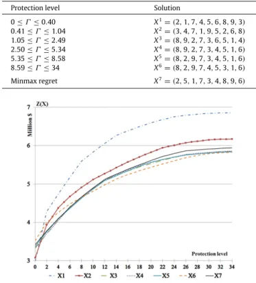
for that instance.

5.3. Illustrative example

The quality of the robust solutions are examined in this subsection. For this purpose, we compare the solutions of the RQAP model for an uncertain QAP withn

=

9. Thef+_,f−_anddmatrices are presented inTable 1. This example has

|

J

| =

34 uncertain flows. The solutions of RQAP for all values ofΓ

∈ [

0

,

34

]

are presented in

Table 2. In this table,X7_{is the minmax regret solution. In addition,}

Opt

(

f−

)

=

_X1_,Opt

(

_f=

)

=

_X4_{, andOpt}

(

_f+

)

=

_X6_.

Fig. 1depicts robust cost,Z

(

X

)

, of solutionsX1

, . . . ,

X7versus

Γ

∈ [

0

,

34

]

. In this figure, it is clear which assignment has the best (minimum) robust cost for each value ofΓ. Note thatZ

(

X

)

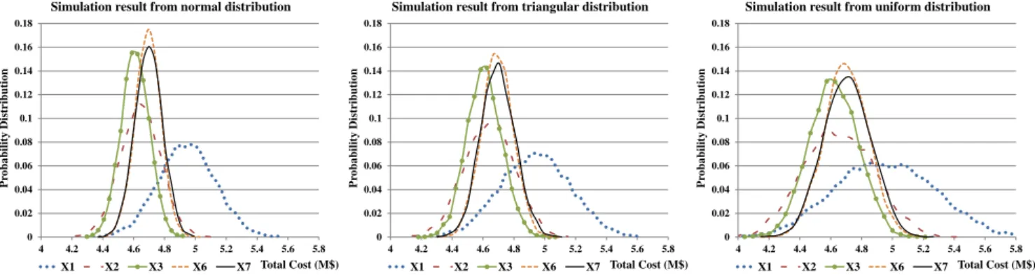
ofX4

andX5_{are very similar toX}3_{. Therefore, for clarity of the graphs in}

Fig. 2, the graphs corresponding toX4andX5are omitted. For 10,000 runs we generated uncertain flowfij,

∀

(

i

,

j

)

∈

J, and

simulated total cost. For this purpose, we used truncated normal, symmetric triangular, and uniform distributions in

[

f−

,

_f+

]

_to gen-erate random flows. The results of the simulations are presented inTable 3and Fig. 2. LetC

(

X

)

= ⟨

f

,

X

⟩

be the random cost of assignmentX, which depends on the realization off. InTable 3,

E

(

C

(

X

))

and

σ (

C

(

X

))

are empirical estimations of the expectation and standard deviation ofC

(

X

)

, respectively. Moreover,C0.95

(

X

)

andC0.99

(

X

)

are the 0.95 and 0.99 quantiles ofC

(

X

)

, respectively.

Cmax

(

X

)

is the maximum observedC

(

X

)

in the simulation. For all

three simulated distributions,X4_andX6_{have the leastE}

(

_C

(

_X

))

_and

σ (

C

(

X

))

, respectively.X4has also the leastC0.95

(

X

)

for normal and

Table 1

Input data of the illustrative example. Matrixf+ Matrixf− Matrixd 1 2 3 4 5 6 7 8 9 1 2 3 4 5 6 7 8 9 1 2 3 4 5 6 7 8 9 1 0 518 0 0 0 624 491 915 0 0 147 0 0 0 296 379 681 0 0 604 657 830 280 795 1340 246 593 2 518 0 577 0 0 0 183 0 0 147 0 94 0 0 0 122 0 0 604 0 515 544 404 633 1430 358 223 3 0 577 0 0 0 360 0 0 0 0 94 0 0 0 290 0 0 0 657 515 0 173 457 138 915 411 738 4 0 0 0 0 0 410 0 0 138 0 0 0 0 0 336 0 0 131 830 544 173 0 630 89 886 584 767 5 0 0 0 0 0 565 760 0 403 0 0 0 0 0 191 474 0 154 280 404 457 630 0 595 1060 130 593 6 624 0 360 410 565 0 217 0 683 296 0 290 336 191 0 25 0 547 795 633 138 89 595 0 797 549 856 7 491 183 0 0 760 217 0 128 592 379 122 0 0 474 25 0 6 302 1340 1430 915 886 1060 797 0 1190 1653 8 915 0 0 0 0 0 128 0 54 681 0 0 0 0 0 6 0 40 246 358 411 584 130 549 1190 0 463 9 0 0 0 138 403 683 592 54 0 0 0 0 131 154 547 302 40 0 593 223 738 767 593 856 1653 463 0 Table 2

Optimal solutions of the example for different protection levels. Protection level Solution

0≤Γ ≤0.40 X1_{=(2,1,7,4,5,6,8,9,3)} 0.41≤Γ≤1.04 X2_{=(3,4,7,1,9,5,2,6,8)} 1.05≤Γ≤2.49 X3_{=(8,9,2,7,3,6,5,1,4)} 2.50≤Γ≤5.34 X4_{=(8,9,2,7,3,4,5,1,6)} 5.35≤Γ≤8.58 X5_{=(8,2,9,7,3,4,5,1,6)} 8.59≤Γ≤34 X6_{=(8,2,9,7,4,5,3,1,6)} Minmax regret X7_{=(2,5,1,7,3,4,8,9,6)}

Fig. 1. Robust cost of assignmentsx1_{, . . . ,x}7_{versus protection levelΓ.} minimumC0.99

(

X

)

andCmax

(

X

)

for normal and triangular

distri-butions, respectively. It has also the leastC0.95

(

X

)

andC0.99

(

X

)

for

uniform distribution. MinimumCmax

(

X

)

for normal and uniform

distributions is found forX5_{. AlthoughOpt}

(

_f+

)

=

_X6_,X6_{did not}

provide the minimumCmax

(

X

)

for any of the simulated

distribu-tions.

According to the results inTable 3andFig. 2, assignmentsX3_,

X4andX5outperform the other assignments almost in all of the metrics and distributions. As illustrated in this example, RQAP with budgeted uncertainty provides a pool of robust assignments depending on the value ofΓ. Then, the decision makers can pick one of these assignments based on their risk preferences.

5.4. Numerical results

In this subsection, we present the extensive results of imple-menting the proposed robust methods on ‘‘easy’’, ‘‘moderate’’ and ‘‘hard’’ instances. Recalling from Section4, each of the proposed exact and heuristic methods for RQAP provides an upper bound for optimal robust cost of RQAP. LetubEX,ub2OandubTSbe the

up-per bounds obtained by Exact, 2-Opt and tabu search, respectively.

Note that only the Exact method provides lower bounds, which we denote bylbEX. We definegapEXas

gapEX

=

ubEX

−

lbEX

ubEX

×

100

.

Table 4reports CPU time in seconds spent by CPLEX on Exact

method to solve MIP model(24)–(27). This time is denoted bytEX.

|

J

|

indicates the number of uncertain flows. In all of these instances, Exact method was able to find the optimal solution, i.e.gapEX

=

0

andubEX

=

lbEXfor all easy instances.

According toTable 4, for almost all easy instances, increasingΓ results in a significant increase intEX. This observation is also true

for moderate instances inTable 10. That means that increasingΓ loosens linearization(24)–(27)for RQAP.

By comparing tEX in Table 4 with the time spent to obtain

minmax regret solutions (Tables 2 and 3 in [45]), it is observed that even for large values ofΓ,tEXis about 10%–30% of minmax regret

solution time for most of the easy instances.

Table 5presents the CPU time in seconds spent on 2-Opt (t2O)

and tabu search (tTS) to heuristically solve RQAP for easy instances.

UnliketEX, increasingΓ did not affectt2OandtTS systematically.

Therefore, for moderate and hard instances, we only report average CPU times for different values ofΓ.

To assess the quality of solutions obtained from heuristics, we usedub2OandubTS, upper bounds from heuristics, andlbEX, the best

lower bound from the Exact method. We definedgap2OandgapTSas

gap2O

=

ub2O

−

lbEX ub2O

×

100 and gapTS

=

ubTS

−

lbEX ubTS

×

100

.

In group chr15c, forΓ

=

1

,

2

,

8 and 16 thegapTSwas 0.01%, 0.08%,

0.06% and 0.47%, respectively. This gap for chr15b andΓ

=

8 was 0.04%. For the rest of cases, tabu search found the optimal robust solutions. For chr15c andΓ

=

1

,

2

,

4

,

8 and 16,gap2Owas 0.01%,

0.03%, 0.33%, 0.52% and 0.12%, respectively. This gap for chr15a and

Γ

=

1

,

2

,

4 and 8 was 0.10%, 0.07%, 0.24% and 0.38%, respectively. Moreover,gap2O

=

0

.

18% for chr12c andΓ

=

8. For the rest of

cases, 2-Opt found the optimal robust solutions.

Tables 6–11represent the numerical results for moderate

in-stances. For each group andΓ,Table 6shows the number of in-stances (out of 10) which were solved optimally by Exact method within 7,200 s. Some moderate instances were not solved opti-mally, and a positive optimality gap remained for these cases.

Table 7reports the average optimality gap (among 10 instances)

for each group andΓ.Tables 8and9present the number (in thou-sands) of all nodes and the remaining nodes, respectively, in the branch-and-cut tree explored by CPLEX.

In all of the moderate instances,ub2O

=

ubTS

≤

ubEX. In other

words, the exact method was not able to outperform the heuris-tics in any of the moderate instances. Moreover, in all of these instances, 2-Opt and tabu search got the same solutions, which outperform the solutions of Exact method.

Table 10reportstEXfor moderate instances.t2OandtTSfor these

Fig. 2. Probability distributions of total cost for assignmentsx1_,x2_,x3_,x6_{, andx}7_{in simulation results from normal, triangular, and uniform distributions for uncertain}

material flows. Table 3

Summary of the simulation for assignmentsx1_-x7_{from normal, triangular, and uniform distributions.}

Results from truncated normal distribution Results from symmetric triangular distribution Results from uniform distribution

X E(C(X)) σ (C(X)) C0.95(X) C0.99(X) Cmax(X) E(C(X)) σ(C(X)) C0.95(X) C0.99(X) Cmax(X) E(C(X)) σ(C(X)) C0.95(X) C0.99(X) Cmax(X)

X1 _{4925943 183732 5231124 5353466 5593676 4918265 225385 5287349 5429806 5654092 4922488 318317 5450792 5633086 5983884} X2 _{4625630 130569 4840172 4931579 5068223 4621308 161304 4887201 4984846 5196267 4623809 225544 4996801 5131568 5374541} X3 _{4591398 91583 4741441 4801663 4917547 4587817 113873 4778583 4855632 5044375 4592330 157627 4853489 4941902 5160347} X4 _{4588999 92627 4740427 4803665 4913413 4585379 115035 4778064 4852616 5047118 4590022 159355 4854413 4944834 5170011} X5 _{4606422 89165 4753007 4812793 4913326 4603112 111119 4788751 4863401 5048748 4607485 153171 4860528 4947754 5154671} X6 _{4674114 83334 4809191 4868794 4992954 4671868 102937 4840905 4907941 5108466 4672872 143334 4906776 5003099 5161551} X7 _{4678934 89033 4824954 4881580 4990871 4675413 110900 4860870 4934662 5081722 4679470 153151 4931791 5026293 5235742} Table 4

CPU time spent on the Exact method (tEX) for easy instances.

Protection levelΓ Group |J| 1 2 4 8 16 32 64 chr12a 22 2 4 6 9 18 – – chr12b 22 0.6 0.9 1 1.7 2.4 – – chr12c 22 6 6 8 14 22 – – chr15a 28 39 36 49 90 123 – – chr15b 28 7 8 11 24 38 – – chr15c 28 53 81 129 362 579 – – esc16a 76 33 15 31 56 184 278 235 esc16d 42 17 31 26 26 28 34 – esc16e 42 1.1 1.1 1.3 1.5 1.8 1.8 – esc16g 42 2 2.1 3 4 7 8 – esc16i 30 2 2 2.2 2.1 1.7 – – esc16j 24 0.3 0.3 0.4 0.4 0.4 – – ER07 20 0.1 0.2 0.3 0.4 0.6 – – ER08 29 0.5 0.5 0.7 1.2 2.5 5 – ER09 31 2.3 3 4 7 11 22 – ER10 43 10 12 20 32 65 169 – ER11 55 83 95 114 129 235 647 2865 scr12 56 8 10 10 15 30 68 – tai10a 90 41 46 54 67 115 175 397 tai10b 90 5 7 8 8 11 15 15 tai12b 127 11 12 13 17 24 17 13 teff

2O (tTSeff) and the effective iteration iter eff 2O(iter

eff

TS) for 2-Opt (tabu

search), which are the time and iteration count of discovering the best solution in these algorithms, are reported in this table. We see that the robust cost was not improved by 2-Opt or tabu search after their effective time and iteration count. Based on the results in

Table 11,t_2Oeffandt_TSeffare almost 5% oft2OandtTS, respectively. Note

thatt2O andtTS depend on iteration limits that we set for 2-Opt

and tabu search, respectively. Similarly, we denoted the number of effective restarts in tabu search by Restarteff_2O.

Hard instances were solved heuristically by 2-Opt and tabu search methods for all values of the protection levelΓ

∈ {

1

,

2

,

4

,

8

,

16

,

32

,

64

,

128

,

256

}

such thatΓ

≤

Γ_max, and the results are reported inTable 12. We omitted Exact method for these instances, because there was no hope to solve them exactly. For these cases,

we reportedgap#_2Oandgap#_TSinTable 12which are defined as

gap#_2O

=

ub2O

−

min

{

ub2O

,

ubTS

}

ub2O

×

100

,

and gap#_TS

=

ubTS

−

min

{

ub2O

,

ubTS

}

ubTS

×

100

.

Note that for the cases with the same value ofn, increasing

|

J

|

results in a significant increase int_2Oandt_TS. This is because, in each iteration of 2-Opt and tabu search, computing∆2_abfor each pair of facilitiesa

,

b

∈

Nin(31)requires sorting a vector of length

|

J

|

.

Recalling from Section5.2, we used an iteration limit of 100

×

n2

for tabu search and 10

×

n2restarts for 2-Opt. With this setting, according toTables 11and12, for most of the moderate and hard instances,t2O and tTS are very close to each other. But, tTSeff and

itereff_TSare almost half ofteff 2Oand iter

eff

2O, respectively, in most cases.

Furthermore, based on the values ofgap#_2Oandgap#_TSinTable 12, for most hard instances, the quality of solutions obtained from tabu search is better than 2-Opt.

By comparing t2O and tTS in Table 12, with the time spent

to obtain approximate minmax regret solutions (Tables 6 and 7 in [45]), it is observed thatt2OandtTSare about 10%–30% of minmax

regret solution time for most hard instances.

6. Conclusions and future research

We studied the robust quadratic assignment problem where uncertain interfacility flows belong to a budgeted uncertainty set. Unlike minmax regret QAP, in the robust optimization approach with budgeted uncertainty framework, finding the worst-case scenario and evaluating the robust cost of a given assignment can be done in polynomial time. Therefore, the proposed heuristic and exact methods for RQAP in this paper are significantly faster than heuristic and exact methods, respectively, for minmax regret QAP. Moreover, the robust approach with budgeted uncertainty has an adjustable conservativeness, and the decision maker can get a pool of solutions with different levels of conservativeness. The main contributions of the paper are as follows:

Table 5

CPU time spent on 2-Opt (t2O) and tabu search (tTS) for easy instances. Protection levelΓ

t2O(s) tTS(s)

Group 1 2 4 8 16 32 64 Avg 1 2 4 8 16 32 64 Avg

chr12a 1.2 1.3 1.1 1.1 1.2 – – 1.2 1.5 1.4 1.4 1.4 1.6 – – 1.5 chr12b 1.3 1.3 1.1 1.2 1.4 – – 1.3 1.5 1.5 1.4 1.5 1.6 – – 1.5 chr12c 1.2 1.2 1.1 1.1 1 – – 1.1 1.5 1.4 1.4 1.3 1.4 – – 1.4 chr15a 5 4.7 4.3 4.9 4.7 – – 4.7 4.4 4.2 4.2 4.4 4.4 – – 4.3 chr15b 4.4 5.1 5.1 4.6 4.8 – – 4.8 4.4 4.7 5 4.6 4.4 – – 4.6 chr15c 4.2 3.8 4 4.2 4.1 – – 4.1 4 4.3 4.1 4.8 4.7 – – 4.4 esc16a 11 11 12 11 11 11 12 11 16 15 15 15 15 16 16 15 esc16d 6.8 6.8 6.5 7.1 6.7 6.5 – 6.7 8.1 7.8 8.6 8.1 8.7 7.7 – 8.2 esc16e 5.9 6 5.8 5.9 5.3 5.8 – 5.8 8.5 8.6 8.2 9.2 8.3 8.6 – 8.6 esc16g 5.1 4.9 5.1 5.7 5.1 5.5 – 5.2 7.7 7.3 8.2 8.9 8.4 8.5 – 8.2 esc16i 3.6 3.8 3.6 3.5 3.6 – – 3.6 5.6 6.2 5.9 5.7 6.2 – – 5.9 esc16j 2.9 2.6 2.9 2.8 2.7 – – 2.8 5.2 5.1 5.4 5.6 5.5 – – 5.4 ER07 0.05 0.05 0.05 0.05 0.05 – – 0.05 0.1 0.1 0.1 0.1 0.1 – – 0.1 ER08 0.1 0.1 0.1 0.1 0.1 0.2 – 0.1 0.2 0.2 0.2 0.2 0.2 0.3 – 0.2 ER09 0.3 0.3 0.3 0.3 0.3 0.3 – 0.3 0.5 0.4 0.5 0.5 0.5 0.6 – 0.5 ER10 0.9 0.8 0.8 1 0.9 0.9 – 0.9 1.3 1.3 1.2 1.4 1.3 1.3 – 1.3 ER11 1.9 1.8 1.7 2.1 2 2 2.7 1.9 2.5 2.3 2.3 2.7 2.4 2.7 3.3 2.5 scr12 2.7 2.8 2.8 2.5 2.8 2.8 – 2.7 3.3 3.5 3.7 3.1 3.7 3.8 – 3.5 tai10a 1.9 1.8 1.8 1.7 1.9 1.8 1.8 1.8 3.2 3.1 3.1 2.9 3.2 3.1 3.1 3.1 tai10b 1.9 2 1.9 1.9 1.8 1.7 1.9 1.9 2.8 3 2.9 2.9 2.7 2.6 2.9 2.8 tai12b 7.1 8.2 7.9 7.8 8.1 7.7 7.5 7.7 8.9 9.3 9.1 9 9.1 8.4 8.6 8.9 Table 6

Number of optimally solved moderate instances by the exact method. Protection levelΓ Group |J| 1 2 4 8 16 32 64 128 chr18b 34 10 10 10 8 3 1 – – had12 132 10 10 10 10 9 8 0 0 nug12 132 10 10 10 10 10 6 0 1 rou12 132 10 10 10 10 10 6 0 0 ER12 67 10 10 10 10 10 8 – – ER13 73 9 9 9 9 7 3 0 – tai12a 132 10 10 10 10 10 8 1 0 Table 7

Optimality gap (%) for moderate instances using exact method. Protection levelΓ Group 1 2 4 8 16 32 64 128 chr18b 0 0 0 0.21 6.1 11.6 – – had12 0 0 0 0 0.2 1.1 15.2 26.6 nug12 0 0 0 0 0 1.1 12.5 12.1 rou12 0 0 0 0 0 2.4 12.9 19.9 ER12 0 0 0 0 0 0.14 – – ER13 0.08 0.17 0.24 0.68 1.7 7 18.8 – tai12a 0 0 0 0 0 0.81 7.9 13.9 Table 8

Number of all branch-and-cut nodes (in thousands) for moderate instances. Protection levelΓ Group 1 2 4 8 16 32 64 128 chr18b 5.7 8.8 87 826 1720 2078 – – had12 206 195 222 337 490 907 956 501 nug12 361 403 536 629 864 1277 1009 1077 rou12 342 402 438 565 788 1080 893 825 ER12 241 218 203 297 551 1359 – – ER13 1191 1349 1407 1396 1491 1705 1360 – tai12a 308 327 376 372 570 838 891 864

1. A mathematical programming formulation of the RQAP under budgeted uncertainty.

2. A linearized MIP formulation for RQAP which was solved by CPLEX as an exact method.

3. Two heuristic methods (2-Opt and tabu search) to solve RQAP. 4. Extensive experimental results.

Table 9

Number of remaining branch-and-cut nodes (in thousands) for moderate instances. Protection levelΓ Group 1 2 4 8 16 32 64 128 chr18b 0 0 0 110 861 1395 – – had12 0 0 0 0 84 176 814 465 nug12 0 0 0 0 0 107 575 631 rou12 0 0 0 0 0 221 581 691 ER12 0 0 0 0 0 23 – – ER13 55 107 93 220 389 897 1105 – tai12a 0 0 0 0 0 104 400 610 Table 10

CPU time spent on Exact method (tEX) for moderate instances. Protection levelΓ Group 1 2 4 8 16 32 64 128 chr18b 28 42 225 2245 5797 6948 – – had12 610 613 737 1136 1760 4140 7200 7200 nug12 971 1088 1486 2052 3325 5558 7200 7047 rou12 960 1179 1370 1833 3264 5673 7200 7200 ER12 419 364 391 613 1209 4300 – – ER13 2307 2494 2965 3052 3920 6198 7200 – tai12a 955 985 1124 1167 2307 4209 7096 7200 Table 11

Heuristic results for moderate instances.

2-Opt tabu search

Group t2O teff 2O iter eff 2O Restart eff 2O tTS tTSeff iter eff TS chr18b 11.1 0.62 1605 165 11.7 0.31 932 had12 9.3 0.37 454 71 7.1 0.22 325 nug12 9 0.93 1234 214 6 0.65 1009 rou12 9.3 0.49 592 99 6.7 0.25 356 ER12 4.7 0.06 171 23 4 0.13 391 ER13 6.9 0.17 338 41 6.6 0.19 457 tai12a 9.9 0.54 663 110 7.1 0.21 302

The main conclusions are as follows:

1. The Exact method is well-suited for easy instances (e.g. in-stances withn

≤

11).

2. In the Exact method, CPU time significantly increases by increasing the protection levelΓ.

Table 12

Experimental results for hard instances.

2-Opt tabu search

Group |J| Γmax t2O t2Oeff iter eff 2O Restart eff 2O gap # 2O tTS t eff TS iter eff TS gap # TS esc16b 184 128 39 0.5 274 34 0 43 0.3 164 0 esc16c 101 64 20 0.3 332 41 0 22 0.2 220 0 esc16h 229 128 55 0.4 155 17 0 54 0.5 221 0 had14 181 128 24 1.8 1120 139 0 26 0.7 530 0 had18 305 256 137 40 9770 947 0.07 120 11 2692 0 lipa20a 368 256 262 133 21017 1999 0.39 222 82 14634 0.01 lipa20b 358 256 242 117 20583 1931 0.73 210 43 8068 0.02 nug14 181 128 18 3.2 2433 340 0.03 22 1.7 1342 0 nug15 210 128 29 8.3 4960 640 0.12 32 3.3 2269 0 nug16a 240 128 45 15 7315 887 0.28 48 6.5 3496 0 nug16b 238 128 42 16 8079 985 0.34 45 5.6 3175 0 nug17 272 256 68 27 10182 1147 0.45 68 11 4721 0.01 rou15 210 128 29 7.4 4513 584 0.02 32 2.6 1836 0 rou20 378 256 245 128 22702 2098 0.74 205 58 11232 0.01 ER15 108 128 22 1 1012 102 0 20 0.8 908 0 ER20 192 128 177 24 8126 541 0 112 12 4109 0 ER25 291 256 802 238 37447 1850 0.03 378 69 11321 0 ER30 432 256 3671 1608 104384 3940 0.08 1351 305 20199 0.01 scr15 84 64 12 0.8 1448 150 0 11 1 2012 0 scr20 124 64 83 24 15921 1149 0.04 56 9.2 6509 0 tai15a 208 128 37 10 4909 625 0.02 42 4 2212 0 tai15b 210 128 42 2.3 1210 116 0 38 0.8 480 0 tai17a 266 256 81 35 10429 1206 0.32 84 17 5758 0 tai20a 374 256 239 127 22472 2128 0.94 208 59 11260 0.01 tai20b 380 256 262 117 24728 1775 1.47 176 57 12832 0.01

3. In 2-Opt and tabu search, for the cases with the same n, CPU times significantly increase by increasing the number of uncertain flows

|

J

|

.

4. In all moderate instances, 2-Opt and tabu search methods outperformed the Exact method.

5. In most hard instances, in the same time and number of iterations, tabu search outperformed 2-Opt. Thus, tabu search is recommended for larger instances.

A possible direction for future research may be developing tighter formulations for the linear equivalent of RQAP. Moreover, researchers can design other heuristic methods to solve RQAP and compare the results with 2-Opt and tabu search.

References

[1]Koopmans TC, Beckmann M. Assignment problems and the location of economic activities. Econometrica 1957;25:53–76.

[2]Lawler EL. The quadratic assignment problem. Manage Sci 1963;9(4):586–99. [3]Pierskalla WP. The multi-dimensional assignment and quadratic assignment problems. In: Technical memorandum no. 93. OH: Case Western Reserve Uni-versity, Operations Research Department, School of Management Cleveland; 1967.

[4]Mezmaz M, Mehdi M, Bouvry P, Melab N, Talbi E-G, Tuyttens D. Solving the three dimensional quadratic assignment problem on a computational grid. Cluster Comput 2014;17(2):205–17.

[5]Çela E. The quadratic assignment problem: theory and algorithms. 1998. Dordrecht: Kluwer Academic Publishers; 1998.

[6]Burkard RE, Dell’Amico M, Martello S. Assignment problems. Philadelphia: SIAM; 2009. Revised Reprint.

[7]Sahni S, Gonzalez T. P-complete approximation problems. J ACM (JACM) 1976; 23(3):555–65.

[8]Adams W, Waddell L. Linear programming insights into solvable cases of the quadratic assignment problem. Discrete Optim 2014;14:46–60.

[9]Laurent M, Seminaroti M. The quadratic assignment problem is easy for robinsonian matrices with toeplitz structure. Oper Res Lett 2015;43(1):103–9. [10]Muenvanichakul S, Charnsethikul P. The approximated dynamic programming approach to the dynamic quadratic assignment problem. Thammasat Int J Sci Tech 2007;12(2).

[11]Ahmed ZH. Experimental analysis of crossover and mutation operators on the quadratic assignment problem. Ann Oper Res 2015;1–19.

[12]Tosun U, Dokeroglu T, Cosar A. A robust island parallel genetic algorithm for the quadratic assignment problem. Int J Prod Res 2013;51(14):4117–33. [13]Tosun U. On the performance of parallel hybrid algorithms for the solution of

the quadratic assignment problem. Eng Appl Artif Intell 2015;39:267–78. [14]Zhang Q, Sun J, Tsang E, Ford J. Estimation of distribution algorithm with

2-opt local search for the quadratic assignment problem. In: Towards a new evolutionary computation. Springer; 2006. p. 281–92.

[15]Dokeroglu T. Hybrid teaching–learning-based optimization algorithms for the quadratic assignment problem. Comput Ind Eng 2015;85:86–101.

[16]De Klerk E, Sotirov R. Exploiting group symmetry in semidefinite programming relaxations of the quadratic assignment problem. Math Program 2010;122(2): 225–46.

[17]Peng J, Zhu T, Luo H, Toh K-C. Semi-definite programming relaxation of quadratic assignment problems based on nonredundant matrix splitting. Comput Optim Appl 2015;60(1):171–98.

[18]Kaufman L, Broeckx F. An algorithm for the quadratic assignment problem using Bender’s decomposition. Eur J Oper Res 1978;2(3):207–11.

[19]Xia Y, Yuan Y-X. A new linearization method for quadratic assignment problems. Optim Methods Softw 2006;21(5):805–18.

[20]Nyberg A, Westerlund T. A new exact discrete linear reformulation of the quadratic assignment problem. Eur J Oper Res 2012;220(2):314–9. [21]Nyberg A, Westerlund T, Lundell A. Improved discrete reformulations for the

quadratic assignment problem. In: Integration of AI and OR techniques in constraint programming for combinatorial optimization problems. Springer; 2013. p. 193–203.

[22]Zhang H, Beltran-Royo C, Ma L. Solving the quadratic assignment problem by means of general purpose mixed integer linear programming solvers. Ann Oper Res 2013;207(1):261–78.

[23]Hahn PM, Zhu Y-R, Guignard M, Hightower WL, Saltzman MJ. A level-3 reformulation-linearization technique-based bound for the quadratic assignment problem. INFORMS J Comput 2012;24(2):202–9.

[24]Rostami B, Malucelli F. A revised reformulation-linearization technique for the quadratic assignment problem. Discrete Optim 2014;14:97–103.

[25]De Klerk E, Marianna E, Sotirov R, Truetsch U, et al. Symmetry in rlt-type relaxations for the quadratic assignment and standard quadratic optimization problems. Eur J Oper Res 2014;233(3):488–99.

[26]Zhang H, Beltran-Royo C, Constantino M. Effective formulation reductions for the quadratic assignment problem. Comput Oper Res 2010;37(11):2007–16. [27]Fischetti M, Monaci M, Salvagnin D. Three ideas for the quadratic assignment

problem. Oper Res 2012;60(4):954–64.

[28]Steinberg L. The backboard wiring problem: A placement algorithm. SIAM Rev 1961;3(1):37–50.

[29]Geoffrion AM, Graves G. Scheduling parallel production lines with changeover costs: Practical application of a quadratic assignment/LP approach. Oper Res 1976;24(4):595–610.

[30]Heffley DR. The quadratic assignment problem: A note. Econometrica 1972; 1155–63.

[31]Pollatschek M, Gershoni N, Radday Y. Optimization of the typewriter keyboard by simulation. Angew Inform 1976;17(0):438–9.

[32]Dickey J, Hopkins J. Campus building arrangement using topaz. Transp Res 1972;6(1):59–68.

[33]Elshafei AN. Hospital layout as a quadratic assignment problem. Oper Res Q 1977;28(1):167–79.

[34]Francis RL, White JA, McGinnis LF. Facility layout and location: an analytical approach. vol. 31. NJ: Prentice-Hall Englewood Cliffs; 1974.

[35]Alkaya AF, Duman E. Combining and solving sequence dependent traveling salesman and quadratic assignment problems in PCB assembly. Discrete Appl Math 2015.

[36]Loiola EM, de Abreu NMM, Boaventura-Netto PO, Hahn P, Querido T. A survey for the quadratic assignment problem. Eur J Oper Res 2007;176(2):657–90.

[37]Hahn PM, Zhu Y-R, Guignard M, Smith JM. Exact solution of emerging quadratic assignment problems. Int Trans Oper Res 2010;17(5):525–52.

[38]Drezner Z. The quadratic assignment problem. In: Location science. Springer; 2015. p. 345–63.

[39]Feizollahi MJ, Modarres M. Robust quadratic assignment problem with uncertain locations. Iran J Oper Res 2012;3(2):46–65.

[40]Madhusudanan Pillai V, Hunagund IB, Krishnan KK. Design of robust layout for dynamic plant layout problems. Comput Ind Eng 2011;61(3):813–23. [41]Liu L, Li Y. The fuzzy quadratic assignment problem with penalty: New models

and genetic algorithm. Appl Math Comput 2006;174(2):1229–44.

[42]Snyder LV. Facility location under uncertainty: a review. IIE Trans 2006;38(7): 547–64.

[43]Zhao Y, Wallace SW. Integrated facility layout design and flow assignment problem under uncertainty. INFORMS J Comput 2014;26(4):798–808. [44]Feyzollahi M, Shokouhi A, Yazdi MM, Tarokh M. Designing a model for optimal

hospital unit layout. Pejouhandeh 2009;14(4):191–8.

[45]Feizollahi MJ, Averbakh I. The robust (minmax regret) quadratic assignment problem with interval flows. INFORMS J Comput 2014;26(2):321–35. [46]Bertsimas D, Sim M. Robust discrete optimization and network flows. Math

Program 2003;98(1–3):49–71.

[47]Bertsimas D, Sim M. The price of robustness. Oper Res 2004;52(1):35–53. [48]Feizollahi MJ, Modarres M. The robust deviation redundancy allocation

problem with interval component reliabilities. IEEE Trans Reliab 2012;61(4): 957–65.

[49]Soltani R, Sadjadi SJ, Tavakkoli-Moghaddam R. Robust cold standby redun-dancy allocation for nonrepairable series–parallel systems through Min-Max regret formulation and Benders’ decomposition method. Proc Inst Mech Eng O 2014;228(3):254–64.

[50]Feizollahi MJ, Ahmed S, Modarres M. The robust redundancy allocation problem in series-parallel systems with budgeted uncertainty. IEEE Trans Reliab 2014;63(1):239–50.

[51]Feizollahi MJ, Soltani R, Feyzollahi H. The robust cold standby redundancy allocation in series-parallel systems with budgeted uncertainty. IEEE Trans Reliab 2015;64(2):799–806.

[52]Buffa ES, Armour GC, Vollmann TE. Allocating facilities with CRAFT. Harvard University; 1964.

[53]Glover F. Tabu search — part I. ORSA J Comput 1989;1(3):190–206. [54]Glover F. Tabu search — part II. ORSA J Comput 1990;2(1):4–32.

[55]Taillard E. Robust taboo search for the quadratic assignment problem. Parallel Comput 1991;17(4):443–55.