Mechanical Properties of Kenaf Composites Using Dynamic Mechanical Analysis

(1)

Utah State University Utah State University

DigitalCommons@USU

All Graduate Theses and Dissertations Graduate Studies 5-2015

Mechanical Properties of Kenaf Composites Using Dynamic

Mechanical Analysis

Thomas A. Loveless

Follow this and additional works at: https://digitalcommons.usu.edu/etd Part of the Mechanical Engineering Commons

Recommended Citation Recommended Citation

Loveless, Thomas A., "Mechanical Properties of Kenaf Composites Using Dynamic Mechanical Analysis" (2015). All Graduate Theses and Dissertations. 4310.

https://digitalcommons.usu.edu/etd/4310

This Thesis is brought to you for free and open access by the Graduate Studies at DigitalCommons@USU. It has been accepted for inclusion in All Graduate Theses and Dissertations by an authorized administrator of DigitalCommons@USU. For more information, please contact [email protected].

(2)

MECHANICAL PROPERTIES OF KENAF COMPOSITES USING

DYNAMIC MECHANICAL ANALYSIS by

Thomas A. Loveless

A thesis submitted in partial fulfillment of the requirements for the degree

of

MASTER OF SCIENCE in

Mechanical Engineering

Approved:

Dr. Thomas Fronk Dr. Steve Folkman

Major Professor Committee Member

Dr. Marc Maguire Dr. Mark R. McLellan

Committee Member Vice President for Research and

Dean of the School of Graduate Studies UTAH STATE UNIVERSITY

Logan, Utah 2015

(3)

ii

(4)

iii ABSTRACT

Mechanical Properties of Kenaf Composites Using Dynamic Mechanical Analysis by

Thomas A. Loveless, Master of Science Utah State University, 2015 Major Professor: Dr. Thomas Fronk

Department: Mechanical and Aerospace Engineering

Natural fibers show potential to replace glass fibers in thermoset and thermoplastic composites. Kenaf is a bast-type fiber with high specific strength and great potential to compete with glass fibers.

In this research kenaf/epoxy composites were analyzed using Dynamic Mechanical Analysis (DMA). A three-point bend apparatus was used in the DMA testing. The samples were tested at 1 hertz, at a displacement of 10 μm, and at room temperature.

The fiber volume content of the kenaf was varied from 20% - 40% in 5% increments. Ten samples of each fiber volume fraction were manufactured and tested. The flexural storage modulus, the flexural loss modulus, and the loss factor were reported. Generally as the fiber volume fraction of kenaf increased, the flexural storage and flexural loss modulus increased. The loss factor remained relatively constant with increasing fiber volume fraction.

(5)

iv Woven and chopped fiberglass/epoxy composites were manufactured and tested to be compared with the kenaf/epoxy composites. Both of the fiberglass/epoxy composites reported higher flexural storage and flexural loss modulus values. The kenaf/epoxy composites reported higher loss factor values. The specific flexural storage and specific flexural loss modulus were calculated for both the fiberglass and kenaf fiber composites. Even though the kenaf composites reported a lower density, the fiberglass composites reported higher specific mechanical properties.

(6)

v PUBLIC ABSTRACT

Mechanical Properties of Kenaf Composites Using Dynamic Mechanical Analysis by

Thomas A. Loveless, Master of Science Utah State University, 2015

Natural fibers show potential to replace glass fibers. Kenaf is a bast-type fiber with potential to compete with glass fibers

In this research kenaf/epoxy composites were analyzed using Dynamic Mechanical Analysis (DMA). A three-point bend apparatus was used in the DMA testing.

The fiber volume content of the kenaf was varied and ten samples of each fiber volume fraction were manufactured and tested. The mechanical properties of the kenaf composites were reported. Generally as the fiber volume fraction of kenaf increased the mechanical properties increased.

Woven and chopped fiberglass/epoxy composites were manufactured and tested to be compared with the kenaf/epoxy composites. Both of the fiberglass/epoxy composites reported significantly higher mechanical properties. The kenaf/epoxy composites reported higher damping values. The specific mechanical properties were calculated for both the fiberglass and kenaf fiber

(7)

vi composites. Even though the kenaf composites have a lower density, the fiberglass composites reported higher specific mechanical properties.

(8)

vii ACKNOWLEDGMENTS

I would like to thank Dr. Thomas Fronk for giving me the opportunity to work with him on this research. It was an unforgettable opportunity and invaluable to my education at Utah State. I am grateful to the entire faculty at Utah State for teaching me valuable concepts that I was able to apply in this research. I would like to thank Dr. Folkman and Dr. Maguire for serving on my thesis committee. I appreciate the experience and advice they offered me. Special thanks to my fellow graduate students, especially Josh Heil and Cole Blakely, who helped me throughout my schooling and thesis work.

I would like to extend appreciation to the Netzsch staff. They helped work through some of the technical issues we ran into with the DMA. I acknowledge the support from the Microscopy Core Facility at Utah State University for the SEM work. I appreciate the machining work Terry Zollinger did for this research.

I would like to thank my family for supporting me through my schooling career. Special thanks to my brother and my dad for discussing technical information with me regarding my thesis topic. I would like to send special thanks to my wife, Dixie, who put up with me through the ups and downs of the schooling process. I am also thankful for my faith in God, which always served as a firm foundation for me.

(9)

viii CONTENTS Page ABSTRACT ... iii PUBLIC ABSTRACT ... v ACKNOWLEDGMENTS ... vii LIST OF TABLES ...x LIST OF FIGURES ... xi CHAPTER 1. INTRODUCTION ... 1 2. LITERATURE REVIEW ... 3 2.1 Introduction ... 3 2.2 Kenaf ... 3

2.3 Dynamic Mechanical Analysis ... 5

2.4 Material Damping ... 7

2.5 Conclusion ... 8

3. OBJECTIVES ...10

4. DYNAMIC MECHANICAL ANALAYSIS ...11

4.1 Basic Principles ... 11

4.2 Dynamic Mechanical Analysis Deliverables ... 15

4.3 Dynamic Mechanical Analyzer Specifications ... 20

4.4 Dynamic Mechanical Analyzer Calibrations ... 23

4.4.1 Dynamic Mass Calibration ...24

4.4.2 Empty System Calibration ...24

4.4.3 Stiffness Calibration ...24

4.4.4 Rotational Tuning Calibration...25

4.4.5 Temperature Calibration ...25

5. SAMPLE MANUFACTURING ...26

5.1 Kenaf Fiber ... 26

5.2 Sample Mold ... 27

5.3 Percent Volume Content ... 29

5.4 Manufacturing ... 32

5.5 Scanning Electron Microscope Images ... 35

5.6 Sample Surface Preparation ... 39

(10)

ix

6.1 Kenaf Fiber Density ... 42

6.2 Epoxy Matrix Density ... 44

6.3 Fiberglass and Kenaf Composite Density ... 45

7. DYNAMIC MECHANICAL ANALYSIS RESULTS ...53

7.1 Dynamic Mechanical Analysis Frequency Results ... 53

7.2 Epoxy 2050 Resin ... 55

7.3 Woven and Chopped Fiberglass Composites ... 57

7.4 Kenaf Fiber Composites ... 62

7.5 Overall Results ... 72

7.6 Specific Material Properties ... 74

8. UNCERTAINTY ANALYSIS ...77

8.1 Uncertainty Approach ... 77

8.2 Storage and Loss Modulus ... 77

8.3 Volume Uncertainty ... 79

8.4 Specific Storage and Loss Modulus ... 81

8.5 Total Uncertainty ... 82

9. CONCLUSION ...84

9.1 Dynamic Mechanical Analysis ... 84

9.2 Kenaf/Epoxy Composites ... 85

9.3 Recommendations for Future Work ... 86

REFERENCES ...87

APPENDICES ...89

A. Dynamic Mechanical Analyzer Instructions ... 90

(11)

x LIST OF TABLES

Table Page

1. Materials with approximate loss factor values ... 8

2. Aluminum storage modulus tested at 1 hz and 10µm on the DMA ... 19

3. The volume of the fiber for the different fiber volume fractions ... 31

4. Initial kenaf fiber density test ... 43

5. Kenaf fiber density test with bubble removal technique employed ... 43

6. Uncertainty values associated with the DMA governing equation ... 78

7. Uncertainty values for the volume uncertainties ... 80

8. Bias uncertainty values for the specific storage and loss modulus uncertainties ... 81

B9. Chopped glass fiber properties ... 101

B10. Woven glass fiber properties ... 101

B11. 2050 Neat Resin A/B1 ... 102

B12. 20% kenaf fiber composite properties ... 103

B17. Aluminum 7075-T6 material properties tested at 1 hertz ... 105

B18. Aluminum 7075-T6 material properties tested at 0.1 hertz ... 106

(12)

xi

LIST OF FIGURES

Figure Page

1. Force plot at 1 hertz with a static load of 1 N and a dynamic force of 1 N ... 12

2. Displacement plot at 1 hertz with a displacement of 10 μm and a static displacement of 10 μm... 12

3. Force plot at 1 hertz and a static force of 1 N. The figure shows the applied force and the material response. ... 13

4. Force plot at 1 hertz and a static force of 1 N, perfectly elastic solid. ... 14

5. Force plot at 1 hertz and a static force of 1 N, perfectly viscous response. ... 14

6. Simply supported sample, representing the three-point bend sample holder ... 21

7. Netzsch DMA calculator used in the experiment design phase. ... 23

8. Bundle of kenaf fiber used by the composites lab... 26

9. Cutting a small bundle of kenaf into 5 - 10 mm lengths with scissors ... 27

10. Manufactured HDPE mold ... 28

11. Solid Edge drawing of the HDPE mold ... 28

12. C-clamps were added to the mold to induce pressure on the samples ... 30

13. Balance scale used to measure the kenaf fiber ... 32

14. Different amounts of dry fibers in the mold and applying the resin to the mold ... 33

15. PT 2050 part A resin and B1 hardener ... 34

16. Kenaf fiber composites prepared for the Scanning Electron Microscope ... 36

17. Kenaf fiber composite viewed with the SEM, most o the fibers in this image appear to be oriented in the same direction ... 37

(13)

xii

18. Kenaf fiber composite showing the fiber and matrix ... 37

19. Randomly oriented kenaf fiber in epoxy matrix ... 38

20. Void in the kenaf fiber composite ... 38

21. Individual fiber under high magnification with the SEM ... 39

22. Heavy grit sanding station with a kenaf composite being resurfaced ... 40

23. Final sanding station, wet sanding, with a kenaf composite sample... 40

24. Kenaf fiber density average value with 95% uncertainty ... 44

25. Epoxy 2050 A/B1 density ... 45

26. Woven fiberglass 40% fiber volume fraction epoxy resin composite density ... 46

27. Chopped fiberglass 40% fiber volume fraction epoxy resin composite density ... 47

28. Chopped kenaf fiber 20% fiber volume fraction epoxy resin composite density ... 47

29. Chopped kenaf 25% fiber volume fraction epoxy resin composite density ... 48

33. Chopped kenaf density with varying volume fractions ... 50

34. Fiberglass, composite, kenaf composite, and resin densities ... 51

35. Aluminum 7075-T6 flexural storage modulus tested at 10 μm with varying frequencies ... 54

36. Aluminum 7075-T6 flexural loss modulus tested at 10 μm with varying frequencies ... 54

(14)

xiii

38. Flexural Loss Modulus of epoxy 2050 resin ... 56

39. Loss factor of epoxy 2050 resin ... 57

40. Flexural storage modulus of woven fiberglass/epoxy composites ... 58

41. Flexural loss modulus of woven fiberglass/epoxy composites ... 58

42. Loss factor of woven fiberglass/epoxy composites ... 59

43. Flexural storage modulus of chopped fiberglass/epoxy composites ... 59

44. Flexural loss modulus of chopped fiberglass/epoxy composites ... 60

45. Loss factor of chopped fiberglass/ epoxy composites ... 60

46. Average flexural storage modulus of chopped glass and woven glass composites ... 61

47. Average flexural loss modulus of chopped glass and woven glass composites ... 61

48. Average loss factor of chopped glass and woven glass composites ... 62

49. Kenaf composite 20% volume fraction flexural storage modulus ... 63

50. Kenaf composite 20% volume fraction flexural loss modulus ... 63

51. Kenaf composite 20% volume fraction loss factor ... 64

(15)

xiv

64. Kenaf composite flexural storage modulus with varying fiber volume fractions ... 70

65. Kenaf composite flexural loss modulus with varying fiber volume fractions ... 71

66. Kenaf composite loss factor with varying fiber volume fractions ... 71

67. Tested material average flexural storage modulus ... 73

68. Tested material average flexural loss modulus ... 73

69. Tested material average loss factor ... 74

70. Specific storage modulus of kenaf and glass fiber composites ... 75

71. Specific loss modulus of kenaf and glass fiber composites ... 75

A72. DMA software icons ... 90

A73. Opening screen in the Netzsch software for the Dynamic Mechanical Analyzer ... 91

A74. DMA Header information ... 92

A75. DMA Sample Information ... 93

A76. Setup of the initial temperature ... 94

A77. Selection of the initial frequency ... 95

A78. Selection of the test... 96

A79. Isothermal time length end criterion ... 97

A80. Frequency selection ... 98

(16)

xv A82. Final or exit criteria for the DMA ... 100

(17)

CHAPTER 1

1 INTRODUCTION

Natural fibers are a candidate to replace glass fibers in thermoset and thermoplastic composites. There are several advantages of natural fibers over glass fibers. Natural fibers are renewable and cheap to produce, in comparison with the alternatives. Natural fibers have high strength to weight ratios. Natural fiber reinforced composites have been primarily used in applications such as automotive interior linings (BMW i3), upholstery stuffing, and egg boxes. Natural fiber reinforced composites have been limited to non-structural applications [1].

There are several categories of natural fibers. These categories include animal, mineral, and plant or vegetable. The plant or vegetable natural fibers category has several subcategories. These include bast, leaf, seed, and wood. This research is solely interested in looking at kenaf, a bast fiber. Kenaf was chosen because of its high specific mechanical properties.

The mechanical properties of kenaf have been tested and several papers have been published reporting the results. This research includes the testing of kenaf/epoxy composites with Dynamic Mechanical Analysis (DMA). DMA dynamically tests materials for the storage modulus, loss modulus, and the loss factor. A three-point bend apparatus was used to test for the flexural storage modulus and flexural loss modulus. The flexural storage modulus can be compared to the flexural modulus reported from other research, such as the results the

(18)

2 University of Palermo reported [1]. Although the flexural Young’s modulus and the flexural storage modulus are not identical, they are comparable.

The fiber volume fraction of a composite defines how much fiber and resin make up the composite. In this research the fiber volume fraction was controlled from sample to sample. Samples were constructed with 20%, 25%, 30%, 35%, and 40% fiber volume fractions. Woven fiberglass and chopped fiberglass samples were made with 40% fiber volume fraction. These samples, as well as neat resin samples, were used to compare with the kenaf samples. Comparisons included the flexural storage modulus, flexural loss modulus, loss factor, specific flexural storage modulus, and specific flexural loss modulus.

(19)

3 CHAPTER 2

2 LITERATURE REVIEW

2.1 Introduction

The literature review covers important topics that are involved in this research. These include background information on kenaf fibers, the research that has been done with kenaf fibers, a brief description of Dynamic Mechanical Analysis (DMA), how DMA has been used, and material damping. The goal of this literature review is to define what research has been produced on the topics listed above. This will help develop what tests should be done for this research. The literature review reports results that can be compared with the results obtained from this research.

2.2 Kenaf

Kenaf is a warm-season crop that is closely related to cotton. Kenaf has been used in many applications including paper products, building materials, absorbents, and livestock feed. More recently, kenaf has been used in non-structural components in automotive (BMW i3 door panels). Historically kenaf was used in producing twine, rope, and sackcloth. Kenaf has been grown in many countries but was first domestically grown in Northern Africa. During World War II, kenaf crops in the United States increased to help support the war efforts. There is still a lot of room for growth for kenaf as a commercial crop in the United States. However, it will not become established as a commercial crop unless its demand increases.

(20)

4 All natural fibers are cellulosic in nature. The main constituents in biofibers are cellulose and lignin. The strength and stiffness are dependent on the quality and quantity of cellulose [2]. The bark of the kenaf stalk contains long fibers called bast fiber [3]. Kenaf Fibers are extracted from the bast fiber. Filament lengths longer than 1 meter are common. These filaments consist of discrete individual fibers, generally 2-6 mm long. These fibers themselves are composed primarily of cellulose, lignin, and hemicelluloses [4].

Kenaf fibers are being researched to replace glass fibers due to the strength and low density of kenaf. Glass fiber is the dominant fiber used to reinforce thermoset and thermoplastic composites [2]. However, glass fibers require a great deal of energy to produce because processing temperatures can exceed 1200 ˚C [4]. The mechanical properties of kenaf have been researched and vary from study to study. This is most likely due to the non-uniformity of kenaf. Kenaf is not processed like carbon and glass fibers and therefore each individual fiber is very different from the other. The density of kenaf was researched and a range of 1130 kg/m^3 to 1500 kg/m^3 was found.

Kenaf fiber’s mechanical properties were tested by University of Palermo. The tests were performed with a tensile tester and were statistically analyzed due to the high scatter of data. The tensile modulus was found to be around 40 GPa and the ultimate stress was found to be between 350 MPa – 600 MPa. They also tested unidirectional and mat kenaf composites with epoxy resin. The flexural tests reported a flexural modulus of 3.75 MPa for untreated kenaf and 4.2 MPa for treated

(21)

5 kenaf mat composites. As expected, unidirectional kenaf composites reported significantly higher flexural modulus values, around 10 Mpa [1]. The University of Wisconsin also conducted tensile and flexural tests with kenaf. The weight percent of the kenaf fiber varied from 20% to 60% for each test. The flexural modulus varied from around 3 Mpa to 10 Mpa, increasing as the weight percent increased. The tensile modulus followed the same pattern and ranged from 4 Mpa to 12 Mpa. The tensile and flexural strengths were more dependent on whether the composites were coupled or uncoupled. Coupled or uncoupled fibers are treated with a chemical solution. The coupled composites increased steadily for both the tensile and flexural tests as the weight percent increased. The uncoupled composite remained constant with increasing weight percents. The amount of MAPP used on the coupled composites varied between 0% and 3% [4].

2.3 Dynamic Mechanical Analysis

Dynamic mechanical analysis (DMA) is dynamic non-destructive material testing. DMA inputs a sinusoidal force and measures the deflection of the material response to the force. DMA uses the inputted force and material displacement to calculate bulk material properties. The material properties interested in for this research are the flexural storage modulus, flexural loss modulus, and loss factor (tan

δ). The storage modulus is a measurement of materials stiffness, similar to Young’s

modulus. The loss modulus represents the viscous response of the material. This can be defined as the energy lost from the material. The loss factor is simply a ratio of

(22)

6

the loss modulus and the storage modulus. The loss factor is also known as tan δ,

where δ is the phase angle from the sinusoidal input and the material response. The

loss factor is also known as damping.

DMA has the unique capability of being able to vary the frequency throughout a test. This makes it very simple to compare how materials are affected by different frequencies. The temperature can also be changed throughout a test like the frequency. The glass transition temperature can be measured by dynamically changing the temperature and observing the storage modulus, loss modulus, and loss factor. There are three ways to detect the glass transition temperature. The temperature where a spike in the loss factor is found, the point where the loss modulus has a sudden increase before it begins a slow decrease, and at the point where the storage modulus begins to decline [5].

University of Palermo used DMA to study the effects of temperature on both kenaf mat composites and kenaf unidirectional composites. The storage modulus, loss modulus, and loss factor were calculated over a temperature range of 25 ˚C to 140 ˚C. The glass transition temperature was found and compared for the different type of composites that were tested. The tests were conducted at a frequency of 1 hz [1].

Beihang University performed DMA testing on nickel-based superalloy metal rubber (nickel MR). The storage modulus and loss factor of the nickel MR were measured over a frequency range of 0.1 hz to 200 hz. The force and strain were altered over the various tests. As the force and strain were changed the storage

(23)

7 modulus and loss factor were affected. The loss factor decreased as the frequency increased with large force inputs. However, the loss factor increased slightly when the nickel MR was tested with small strains [6].

2.4 Material Damping

An introduction to Mechanical Vibrations explores the importance of material damping. “In the early years of research leading to the design of high pressure steam jetting from nozzles meant large impulse forces on turbine blades. The first blades failed in a matter of hours from fatigue. Damping was one means of decreasing the number of blade oscillations. By changing the alloy composition of the blade material, the damping capacity was increased twentyfold. Aside, it was noted that the dimensionless damping increased with temperature and decreased with frequency”[7]. Viscous damping tends to increase linearly with increasing frequency. Using viscous damping to represent material damping can incur serious error. Robert Steidel continues to explain a possible reason for why material damping decreases with increasing frequency. “If one portion of a structure is stressed differently from another, as occurs in bending, there will be heat flow across grain boundaries dissipating energy and causing damping. At higher frequencies there is no time for heat to flow and damping is less”[8].

Testing at the Goddard Space Flight Center with aluminum in a vacuum showed that the material damping of aluminum is dependent on frequency. The testing showed that as the frequency increased, the damping coefficient of

(24)

8 aluminum decreased [9]. This is consistent with the theory from Robert Steidel’s text. At Beihang University the nickel MR showed as frequency increased the loss factor decreased for high force test.

There are many mechanisms that can produce damping. In the material damping can be produced by heat transfer, lattice dislocations, yielding, and viscoelastic material behavior. Friction and air damping losses can greatly contribute to damping, but are not considered part of material damping.

E-A-R Specialty Composites have values for different material’s loss factors published as displayed in Table 1 [10].

Table 1: Materials with approximate loss factor values

Material Approximate Loss Factor

Aluminum 0.005 – 0.007 Steel 0.05 – 0.10 Neoprene 0.1 Butyl Rubber 0.4 IsoDamp C-1002 Thermoplastic 1.0 2.5 Conclusion

Kenaf/epoxy composites have been tested using a variety of testing procedures. The material properties of the kenaf-epoxy composites are comparable but vary slightly from paper to paper. A temperature scan of kenaf composites was analyzed using DMA. DMA was used in a different paper to analyze nickel MR

(25)

9 throughout a frequency scan. In both cases the storage modulus, loss modulus, and loss factor were obtained.

The loss factor decreases with increasing frequency with relatively large deformations. Table 1 reported different loss factors for common materials. These values can be compared against values in this research.

(26)

10 CHAPTER 3

3 OBJECTIVES

The purpose of this research is to find the flexural storage modulus, flexural loss modulus, and the loss factor of kenaf/epoxy composites with varying fiber volume fractions using Dynamic Mechanical Analysis. In order to fulfill this purpose the following objectives will be completed:

 Understand the principles of Dynamic Mechanical Analysis

 Manufacture kenaf/epoxy composites with varying fiber volume fractions

 Test aluminum with the Dynamic Mechanical Analyzer (DMA) to understand

what parameters to test with

 Manufacture woven fiberglass/epoxy and chopped fiberglass/epoxy

composites with volume fractions of 40%

 Test the kenaf/epoxy composites, the fiber glass/epoxy composites, and neat

resin samples with the DMA

 Compare the results of kenaf/epoxy composites, fiberglass/epoxy

(27)

11 CHAPTER 4

4 DYNAMIC MECHANICAL ANALAYSIS

4.1 Basic Principles

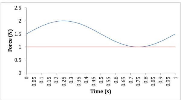
Dynamic Mechanical Analysis (DMA) is non-destructive testing performed to obtain material’s mechanical properties. A specimen is supported in a sample holder apparatus in the DMA. A periodic force is applied to the specimen. There are two ways to control the DMA’s periodic force. Either a target force or a target displacement can be input into the software that controls the DMA. If a target force is selected the DMA will control the force with the load cell. The DMA will record the displacement the push-rod extends under the prescribed force. When a target displacement is selected the DMA will extend the push-rod to that displacement. This is recorded by the displacement sensor which is a Wheatstone bridge type sensor. The DMA will in turn record the force required to extend the push-rod to the displacement. The DMA applies a static load on the sample. Figure 1 and Figure 2 show how the force and displacement correlate with the static preload. However the static load is always applied as a load. Figure 2 shows that the sample is deformed 10 µm under the static preload.

(28)

12

Figure 1: Force plot at 1 hertz with a static load of 1 N and a dynamic force of 1 N

Figure 2: Displacement plot at 1 hertz with a displacement of 10 μm and a static displacement of 10 μm 0 0.5 1 1.5 2 2.5 0 0. 05 _0.1 0. 15 _0.2 0. 25 _0.3 0. 35 _0.4 0. 45 5 _0. 0. 55 _0.6 0. 65 _0.7 0. 75 _0.8 0. 85 _0.9 0. 95 1 For ce (N ) Time (s) 0 5 10 15 20 25 0 0.0 5 0.1 0.1 5 0.2 0.2 5 0.3 0.3 5 0.4 0.4 5 0.5 0.5 5 0.6 0.6 5 0.7 0.7 5 0.8 0.8 5 0.9 0.9 5 1 Di sp la cme n t (μ m) Time (s)

(29)

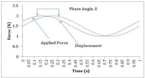
13 When a sample is tested with the DMA two sets of data are recorded. The force and displacement applied and the force and displacement recorded from the material deformation. The force and displacement applied pertain to the elastic properties of the sample. The response of the sample to the deformation pertains to the viscous properties. The in-phase portion corresponds to the elastic nature and

the out-of-phase corresponds to the viscous nature. Figure3 represents the applied

force and the response of the sample to the applied force.

Figure 3: Force plot at 1 hertz and a static force of 1 N. The figure shows the applied force and the material response

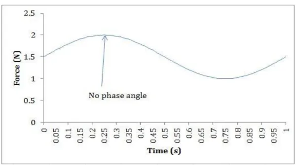
The applied force and the material response would be identical in a perfectly elastic material. In this case the phase angle would be zero, shown in Figure 4. The deformation and response would be 90 degrees out-of-phase for perfectly viscous materials. Figure 5 shows the plot of a perfectly viscous material.

(30)

14

Figure 4: Force plot at 1 hertz and a static force of 1 N, perfectly elastic solid.

Figure 5: Force plot at 1 hertz and a static force of 1 N, perfectly viscous response.

All of the materials tested in this research are viscoelastic and have a phase shift. 0 0.5 1 1.5 2 2.5 0 0. 05 _0.1 0. 15 _0.2 0. 25 _0.3 0. 35 _0.4 0. 45 5 _0. 0. 55 _0.6 0. 65 _0.7 0. 75 _0.8 0. 85 _0.9 0. 95 1 For ce (N ) Time (s)

Phase Angle, δ, 90 degress out-of-phase

(31)

15

4. 1

represents the strain of a viscoelastic material response to a sinusoidal load. Where

represents the strain amplitude, ω represents the angular frequency, δ represents

the phase angle, and represents the static strain.

4. 2

and

_{4. 3}

these two equations are formulated from splitting equation 4.1 and correlating to

the storage strain ε’ and loss strain ε’’. The in-phase portion is the storage strain and

the out-of-phase portion is the loss strain.

4.2 Dynamic Mechanical Analysis Deliverables

Storage modulus, loss modulus, and the loss factor are some of the mechanical properties the DMA can test for. As mentioned in section 4.1 the DMA applies a sinusoidal force or displacement and records the force or displacement of the materials response. The DMA utilizes Hooke’s law to compute the stiffness of the materials. There are several sample holders the DMA can use when testing samples, this is covered in more detail in later sections. In this research and for the following

(32)

16

examples the three-point bend geometry will be used. The equivalent stiffness, ,

for a three-point bend geometry is

4. 4 where I is defined as 4. 5

By inspection it can be seen that by inserting equation 4.5 into equation 4.4 the can be written as

_{4. 6}

For linear springs Hooke’s law is [11]

4. 7

where F is the force and A is the displacement. The variable A is defined as the

displacement because the displacement is equivalent to the amplitude of the

sinusoidal displacement input from the DMA. Plugging in the relationship for

(33)

17

4. 8

The dimensions of the sample are known as the geometric factor, GF

4. 9

The geometric factor is different for each sample holder and as shown in equation 4.8 directly relates to the equivalent stiffness.

The DMA has an in-phase and an out-of-phase force F and displacement

amplitude A. These relate to the in-phase and out-of-phase modulus

4. 10

and

4. 11

Similarly to the strain outlined in the previous section the in-phase portion relates to the storage modulus and the out-of-phase relates to the loss modulus

(34)

18 and

_{4. 13}

where represents the complex modulus.

The storage modulus is a measurement of the stiffness. It is comparable to Young’s modulus but is not the exact same. Young’s modulus is an average of the slope of the linear (elastic) region of a stress-strain plot with a pseudo-static load versus displacement relationship. The storage modulus is equivalent to the slope of the hysteresis curve [12]. DMA testing applies an oscillatory force and is tested dynamically. A test with 7075-T6 aluminum was conducted. The Young’s modulus of this specific material is known to be 71700 MPa. Samples of the aluminum were tested with the DMA at displacement amplitude of 10 µm. The storage moduli of the 10 different samples are displayed in Table 2.

(35)

19 Table 2: Aluminum storage modulus tested at 1 hz and 10µm on the DMA

Sample

ID Storage Modulus (Mpa)

1 70675.3 2 76023.6 3 72221.4 4 72982.3 5 81706.0 6 75587.3 7 75165.0 8 75159.2 9 76312.1 10 71720.5 Average 74755.3 Std Dev 3140.9 Recalculated with Chauvenet's Criterion Average 73983.0 Std Dev 2094.9

The highlighted sample, number 5, was excluded based on Chauvent’s Criterion from Coleman and Steele [13]. The recomputed average was found to be 73983.0 Mpa. The storage modulus can be dependent on the displacement of the test. Different displacements will result in different points along the stress-strain curve and could result in different values for the storage modulus.

The loss modulus is proportional to the energy lost during the cycle. The loss modulus is equivalent to the thickness of the hysteresis curve. The ratio of the loss modulus to the storage modulus is known as the loss factor or the damping of the material. The loss factor is known as tan delta (tangent delta). This is shown by

(36)

20

4. 14

Delta δ is the phase angle discussed in the previous section. The tan delta is an

effective way to show the damping of a given material.

4.3 Dynamic Mechanical Analyzer Specifications

DMA uses the geometry factor GF with relationship to the equivalent stiffness

to calculate the material properties. The three-point bend geometry was utilized

in this research. The DMA has several sample holders depending on the geometry and type of material. These include three-point bend, single and dual-cantilever, shearing, tension, penetration, compression, and ball and cup. The ball and cup holder is different from the others because it is designed to test viscous liquids instead of solids. It has the unique capability to test materials as they cure from liquid to solid. Utah State University has the three-point bend, tension, penetration, compression, and ball and cup sample holders.

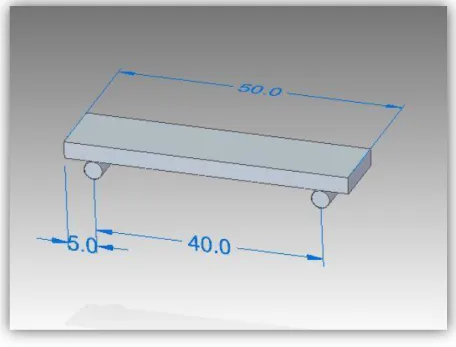
The three-point bend apparatus is effective for stiff materials. Out of the different sample holders the three-point bend requires the least amount of force to deform a sample. Because static force is applied it should not be used with soft materials or with materials that cannot support their own weight. The three-point bend geometry used in this research has a bending span of 40 mm. The maximum height and width of the samples that can be used in the apparatus are 5mm and 12 mm respectively. It is recommended that samples extend 10% of the sample length

(37)

21 past each support of the sample holder [12], Figure 6. Each sample was made to a length of 50 mm to account for the overhang.

Figure 6: Simply supported sample, representing the three-point bend sample holder

The frequency of the periodic force can be varied between tests or during the same tests. The DMA used in this research has the capability of testing between 0.01 and 100 hertz. One advantage of DMA is frequency scans can be done in one test. The DMA cycles through the varying frequencies one frequency at a time. The DMA continually records the displacement, force, and frequency. This makes it possible to compare the material properties to the frequency as the frequency changes throughout the test. When the data is reviewed the software separates the material properties with the corresponding frequency.

(38)

22 The DMA is equipped with a furnace that can heat samples up to 600 ˚C. The heating rates are controllable and the DMA has the capability of heating at rates of 0.01 K/min up to 20 K/min. The DMA has the capability to cool samples as well. A liquid nitrogen Dewar is connected to the DMA’s furnace, this is capable of cooling samples to a temperature of -170 ˚C. Liquid and gaseous nitrogen can be used. This is selected depending on how fast the sample is desired to be cooled. The cooling rates can be controlled up to 10 K/min. The temperature can be changed during the testing. Like the frequency, temperature scans can be done. The mechanical properties can be monitored with relation to the temperature. DMA is often used to find the glass transition temperature using this technique.

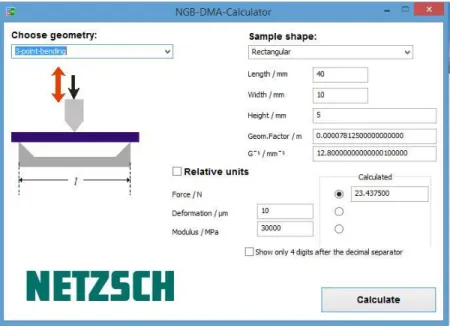
The DMA has a maximum displacement and force of 240 µm and 8 N (7.273 N deliverable). Regardless of whether the test is displacement or force driven both force and displacement will need to be selected below the maximums. The DMA calculator in Figure 7 can be used in the experiment design phase to decide how large a sample should be manufactured and what force or displacement will be required. In this research all of the tests are displacement controlled to a displacement of 10 µm. The DMA calculator was used to decide how big the different samples needed to be for the different materials. In order to use the calculator the size of the sample needs to be input, the deformation or force desired, and the modulus. If the modulus is not known a guess can be inserted. This will get a close enough number that you can proceed with designing a sample size. In the example shown in Figure 7 a sample with a length of 40 mm, width of 10 mm, and a height of

(39)

23 5 mm is analyzed. Note, the 40 mm is a set length because that is the span of the three-point bend apparatus. A displacement of 10 µm is desired for a material with a modulus of 30,000 Mpa. A force of 23.4 N is required to deform the sample. Because the maximum force is 7.273 N the sample would not work at this deformation. The size of the sample would need to be altered. This same process can be done with a test that is controlled by the force.

Figure 7: Netzsch DMA calculator used in the experiment design phase.

4.4 Dynamic Mechanical Analyzer Calibrations

The Netzsch DMA 242 requires several calibrations before tests can be performed. These calibrations are recommended to be done every year and should be done if the equipment is moved or altered. The four calibrations are the dynamic mass calibration, empty system calibration, system stiffness calibration, and

(40)

24 rotation tuning calibration. The calibrations are order specific and are done as listed.

4.4.1 Dynamic Mass Calibration

Dynamic mass calibration is performed with a known mass and without a mass. The known mass is included in the DMA equipment but the mass must be measured and should be measured to a thousandth of a gram. A scale with this fine of resolution is not available in the composites lab. The labs in Biotech have been easy to work with and have allowed us to utilize their scales with better resolution. Both tests are compared and the dynamic system constant is calculated. This calibration is not done with each sample holder.

4.4.2 Empty System Calibration

The empty system calibration is not done with a sample but does require the sample holder to be in place. The empty system calibration steps through different displacement amplitudes and frequencies. It is automatically prompted by the software. The calibration is valid for all sample holders.

4.4.3 Stiffness Calibration

Stiffness calibration tests the internal stiffness of the DMA components at different temperatures and frequencies. The sample holder and stiffness calibration sample are required. The sample is a thick piece of steel that will have infinitesimal deformation with the loads prescribed from the DMA. The test must be done for

(41)

25 each sample holder. Each sample holder has different calibration samples that should be used. The temperature range is selected by the user, if desired the range can include the entire temperature range of the DMA. It is most important to run the calibration for the temperatures that the will be used in the testing of the DMA. This is the longest calibration and is best to run overnight.

4.4.4 Rotational Tuning Calibration

The electronics can add additional noise in the system leading to phase angles that are not related to the material being tested. Assuming that steel has a low loss factor and that the loss factor is linear for the frequency range, the noise from the electronics can be determined. A steel standard is included in the testing equipment to use in this test.

4.4.5 Temperature Calibration

Temperature calibration is performed in order to calibrate the thermocouple the DMA uses to measure the temperature. The calibration will yield a more accurate reading of the thermocouple. Three standard substances are included for the temperature calibration. These substances are adamantan, indium, and lead.

(42)

26 CHAPTER 5

5 SAMPLE MANUFACTURING

5.1 Kenaf Fiber

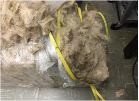
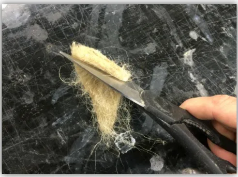
The kenaf fiber is in relatively short lengths and is tangled together as depicted in Figure 8. Because of this characteristic, the manufacturing of the composites was performed with chopped fibers. As shown in Figure 9, the chopped fibers were made by taking a handful of the kenaf fibers and cutting them into 5 – 10 mm lengths using scissors. This method was appropriate with the small size and relatively low number of samples that were required for the DMA testing.

(43)

27

Figure 9: Cutting a small bundle of kenaf into 5 - 10 mm lengths with scissors

5.2 Sample Mold

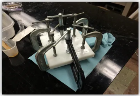
A mold was designed using Solid Edge and built with High Density Polyethylene (HDPE). The Solid Edge model was sent to a machine shop at USU and the machine shop used a CNC router to create the mold precisely as the drawing was illustrated. Figure 10 and Figure 11 compare the drawing with the actual part. HDPE has a low coefficient of friction which made it possible to remove the samples from the mold. The epoxy resin is sticky and will stick to other materials. This can make it very difficult to remove samples from a mold. A water resistant fast-drying silicone spray lubricant was used to further decrease the coefficient of friction of the HDPE.

(44)

28

Figure 10: Manufactured HDPE mold

(45)

29 The mold was designed to produce samples of dimensions 11.1 mm wide and 63.5 mm long. As mentioned in chapter 4 the samples were made to a length of 50 mm. The excess length was necessary because the CNC router was unable to make the ends square. The excess length was trimmed off on each end to make the ends square and cut the samples down to 50 mm. The samples were laid up in the bottom of the mold. The bottom of the mold is shown on the right in Figure 11. The top of the mold has small indentations that match the bottom of the mold. When the top of the mold is laid on top it puts pressure on the sample forcing voids out of the sample. This pressure was also used to compact the sample and force them to the correct height. Figure 12 shows how C-clamps were used to add pressure on the mold. The C-clamps were tightened in a star pattern ensuring good distribution of pressure. Holes were drilled in the top section of the mold for the excess resin and bubbles to exit the sample. As the C-clamps were tightened the excess resin and bubbles came out of the samples.

5.3 Percent Volume Content

Fiber volume content is important in the manufacturing of composites. It has a large impact on the mechanical properties of the composite. Generally, as fiber volume content increases the stiffness and strength of the composite increase. For most applications 60% fiber volume content is a good benchmark for woven and unidirectional fiber composites. Chopped fibers are more difficult to get that high of fiber volume content. The process of making chopped fibers uses more resin and

(46)

30 results in less fiber volume content. In this research fiber volume contents of 20%, 25%, 30%, 35%, and 40% are tested. The fiber volume content was measured and compared for all of the samples. The storage modulus and loss factor (damping) was measured and compared in the results section.

Figure 12: C-clamps were added to the mold to induce pressure on the samples

In order to obtain the desired fiber volume content the kenaf fiber density was researched. The density for kenaf fiber varied from 1130 kg/m^3 to 1500 kg/m^3 in the literature. A density test was conducted and found to be 1024 kg/m^3, more information is available in the density results section. This value for the density was used to determine the fiber volume content. The volume of the composite was known to be 2.2 ml. This was calculated by using the dimensions of the mold used to

(47)

31 manufacture the composites. The fiber volume for the tested fiber volumes are shown in Table 3.

Table 3: The volume of the fiber for the different fiber volume fractions

FiberVolume

Percent Fiber Volume(ml)

20% 0.44

25% 0.55

30% 0.66

35% 0.77

40% 0.88

Using the density and the fiber volume values from Table 3 the values were plugged into

5. 1

where m represents the mass, ρ represents the density, and V represents the

volume. A balance scale shown in Figure 13 was used to weigh a clump of kenaf fiber. Depending on which fiber volume fraction was desired the amount of kenaf would be weighed.

(48)

32

Figure 13: Balance scale used to measure the kenaf fiber

5.4 Manufacturing

The mold described in the previous section had the capability of creating 16 samples. Ten samples were created of each volume fraction, a total of 50 samples. Each time the samples were created, several of each volume fraction were created. This was done in order to get a random assortment of each volume fraction from different manufacturing times, making the comparison between volume fractions more reliable. Figure 14 shows an example of how the different volume fractions were organized in the mold; the top four samples had 20% fiber volume content, the middle four had 30% fiber volume content, and the bottom four had 35% fiber volume content. A space between the different groups of fiber volume contents was

(49)

33 left open. This made the mold easier to work with and allowed for excess resin to drain.

Figure 14: Different amounts of dry fibers in the mold and applying the resin to the mold

The fiber was added to the mold, without any resin. The lower fiber volume contents (20% - 30%) were relatively easy to pack into the mold. The higher fiber volume contents were very difficult to fit into the mold and took a good deal of time to get stuffed into the sample slots. After the dry kenaf fibers were packed into the mold the resin would be prepared. The epoxy resin used in this research was the PT2050 with the B1 hardener, Figure 15.

(50)

34

Figure 15: PT 2050 part A resin and B1 hardener

The PT2050 resin was mixed at a 100% part A to 27% part B mass ratio. This ratio was prescribed by the manufacture, PTM&W. The ratio was obtained by using a digital scale. The resin mixing cup was placed on the scale and zeroed out. The PT2050 resin part A was added to the cup to the desired level. The weight of the resin was noted and the scale was zeroed again. The weight of the resin would be multiplied by 0.27. This is how much B1 hardener would be required. The B1 hardener was added until the weight desired was obtained. It was important to mix the resin thoroughly, making sure all the B1 hardener was mixed into the resin. If the resin was not mixed thoroughly it could lead to inconsistent properties in the

(51)

35 resin. The resin can be considered thoroughly mixed when the color is homogeneous. A syringe was used to add the mixed resin to the kenaf fibers, Figure 14. The resin was added to each sample and rotated throughout all of the samples. The kenaf fibers would soak up the resin so the resin would be applied multiple times. Excess resin was applied so the dry fibers were completely saturated. The resin has a pot-life of one hour. The literature for the resin allows for a minimum of 24 hours before the composite is cured. Before surface preparation was started two days were allowed to ensure full cure of the composites.

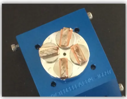
5.5 Scanning Electron Microscope Images

Several composite samples were cut down to be used to photograph using a Scanning Electron Microscope (SEM). The samples dimensions were cut to roughly 11 mm x 3 mm x 3 mm. The samples were cleaned off with acetone. The SEM uses a vacuum and it is important that the samples do not have any loose particles. The loose particles can damage the instrumentation. Because the kenaf composite is not conductive a piece of copper tape was adhered to the sample to help direct the electron beam. Figure 16 shows the four samples that were photographed with the SEM.

(52)

36

Figure 16: Kenaf fiber composites prepared for the Scanning Electron Microscope

The entire cross-sectional surface of each sample was scanned. Figure 17 - through Figure 21 show a variety of the different fiber/epoxy relationships viewed in the samples. Chopped fiber composites are completely random in orientation. As a result some areas of the surface show fibers in a variety of directions. A void can be seen in Figure 20. There was a very low number of voids viewed in the four samples that were photographed.

(53)

37

Figure 17: Kenaf fiber composite viewed with the SEM, most of the fibers in this image appear to be oriented in the same direction

Figure 18: Kenaf fiber composite showing the fiber and matrix

(54)

38

Figure 19: Randomly oriented kenaf fiber in epoxy matrix

(55)

39

Figure 21: Individual fiber under high magnification with the SEM

5.6 Sample Surface Preparation

Surface preparation is important when using the DMA. The calculations the DMA software performs are based on the geometry of the sample. Because of this the geometry needs to be as consistent as possible. The bottom and top surfaces need to be smooth to ensure reliable results. The bottom and top surfaces interact with the DMA pushrod and the three-point bend supports. As stated previously the composites were intentionally made long and needed to be cut to length. The samples could not be shorter than 45 mm and longer than 60 mm. The samples varied from 45 mm – 55 mm. After the ends were cut off the bottom and top surfaces were resurfaced. Two sanding stations were used to resurface the samples, Figure 22 and Figure 23.

(56)

40

Figure 22: Heavy grit sanding station with a kenaf composite being resurfaced

(57)

41 Samples were initially sanded down using the highly abrasive, 120 grit, sandpaper displayed on the left of Figure 22. This first step was intended to make the sample dimensionally consistent. Often times when the samples would be taken out of the mold they would not have consistent dimensions. This step would also remove any large imperfections that may have occurred in the manufacturing process. The sanding station in Figure 23 is a wet sanding station. Running water is piped through the station and runs across the four different grits of sandpaper that are displayed. The sandpaper grits from left to right are 240, 320, 400, and 600. The sample was sanded on each piece of sandpaper for a long enough time to smooth out the scratches made from the previous sandpaper.

(58)

42 CHAPTER 6

6 DENSITY RESULTS

6.1 Kenaf Fiber Density

The literature has varying values for the density of kenaf fiber. Values varied from 1130 kg/m^3 to 1500 kg/m^3 [1] [4] [14] . This is understandable because kenaf is cultivated in different areas of the world and is processed using different techniques. This could result in different density values for kenaf fiber. A density test was performed to calculate the density of the kenaf fiber being used at Utah State University. The water displacement test was used to determine the volume of the kenaf fiber. A simple balance scale, Figure 14, was used to obtain the mass of the kenaf fiber. There were 20 samples with varying amounts of kenaf tested. The first 10 samples were put inside a graduated cylinder full of water and the difference in the volume was recorded, Table 4. It was noted that bubbles formed on the kenaf fibers and would slowly come to the surface. It was apparent that the bubbles were distorting the density values. It was found that using a screwdriver the kenaf fiber could be prodded and the bubbles would come to the surface. After a few minutes of this the bubbles would be completely removed. A test with 10 more samples was conducted using the bubble removal technique. The results are recorded in Table 5. The kenaf fiber is farily uniform but not completely uniform. This could help explain the slight variations in the density. Table 5 represents a significantly lower standard deviation. The bubble removal technique yielded more reliable results. The average

(59)

43 computed for the values depicted in Table 5 was used for this research. Figure 24 shows the average density associated with both density tests.

Table 4: Initial kenaf fiber density test Mass

(grains) Water (ml) Wate

r and Fiber

(ml) Fiber(ml) Volume Density (Kg/m^3)

5.6 18 18.6 0.6 604.8 20.7 19.4 20.4 1 1341.3 28.8 16 19.2 3.2 583.2 28.2 19.6 21.5 1.9 961.8 3 21.8 22.1 0.3 648.0 8.9 18.2 18.9 0.7 823.9 7.4 20.8 21.2 0.4 1198.8 13.5 19.2 21.2 2 437.4 2.7 19.2 19.4 0.2 874.8 Average 830.4 Standard Deviation 299.1

Table 5: Kenaf fiber density test with bubble removal technique employed Mass

grains

Water ml

Water and Fiber ml Fiber Volume ml Density Kg/m^3 2.9 19.2 19.4 0.2 939.6 8.4 20.3 20.8 0.5 1088.6 27.3 20.4 22.2 1.8 982.8 12.8 20.7 21.4 0.7 1184.9 6.3 17.5 17.9 0.4 1020.6 17.8 18 19.3 1.3 887.2 17.6 18.8 20 1.2 950.4 26.1 22 23.6 1.6 1057.0 11.9 20.8 21.6 0.8 963.9 3.4 19.6 19.8 0.2 1101.6 60.5 19.2 22.8 3.6 1089.0 Average 1024.1 Standard Deviation 88.3

(60)

44

Figure 24: Kenaf fiber density average value with 95% uncertainty

6.2 Epoxy Matrix Density

Published data for the density of PT2050 A/B1 resin is available. It was of interest to measure and calculate the density and compare with the published data from the manufacture, 1120 kg/m^3. As mentioned in the resin preparation section the resin is mixed at a 100:27 part A to part B1 mass ratio. Two separate batches of resin were mixed and six samples were made from each batch. This was intended to minimize the effect of user error in mixing the resin. The samples used in the density test were all rectangular cross-section beams. The volume and density were calculated by 6. 1 and 0 200 400 600 800 1000 1200 1400 1600 Average De n si ty (kg /m ^3 ) Initial Test

(61)

45

6. 2

where m is the mass of the sample, V represents the volume, and ρ represents the

density. The mass of each sample was determined using the balance scale, Figure 13. The average density was calculated to be 1106.5 kg/m^3. The results for each sample are displayed in Figure 25.

Figure 25: Epoxy 2050 A/B1 density

6.3 Fiberglass and Kenaf Composite Density

Using the same technique for the neat epoxy the density for the kenaf fiber composites at different volume fractions, woven fiberglass, and the chopped

0 200 400 600 800 1000 1200 1 2 3 4 5 6 7 8 9 10 11 12 D en si ty (k g/ m^3 ) Sample Number

(62)

46 fiberglass composites were determined. Figure 26 through Figure 32 represent the density data for the different materials. In some of the results samples were removed based on Chauvenet’s criterion. For most of the composites 10 samples were manufactured and measured. However, several of the sample groups had more than 10 samples and the chopped fiberglass composites had less than 10 samples.

Figure 26: Woven fiberglass 40% fiber volume fraction epoxy resin composite density 0 200 400 600 800 1000 1200 1400 1600 1800 1 2 3 4 5 6 7 8 9 D en si ty (k g/ m^3 ) Sample Number

(63)

47

Figure 27: Chopped fiberglass 40% fiber volume fraction epoxy resin composite density

Figure 28: Chopped kenaf fiber 20% fiber volume fraction epoxy resin composite density 0 200 400 600 800 1000 1200 1400 1600 1800 1 2 3 4 5 D en si ty ( k g/ m^ 3) Sample Number 0 200 400 600 800 1000 1200 2 3 4 5 6 7 8 9 10 D en si ty (k g/ m^3 ) Sample Number

(64)

48

Figure 29: Chopped kenaf 25% fiber volume fraction epoxy resin composite density

Figure 30: Chopped kenaf 30% fiber volume fraction epoxy resin composite density 0 200 400 600 800 1000 1200 2 3 4 5 6 7 8 9 10 D en si ty (k g/m^3 ) Sample Number 0 200 400 600 800 1000 1200 1 2 4 5 6 7 8 9 10 D en si ty (k g/m ^ 3 ) Sample Number

(65)

49

Figure 31: Chopped kenaf 35% fiber volume fraction epoxy resin composite density

Figure 32: Chopped kenaf 40% fiber volume fraction epoxy resin composite density 0 200 400 600 800 1000 1200 2 3 4 5 6 7 8 9 10 D en si ty (k g/m^3 ) Sample Number 0 200 400 600 800 1000 1200 1 2 4 5 6 7 8 9 10 11 12 13 14 15 16 17 18 D en si ty (k g/m ^ 3 ) Sample Number

(66)

50 The densities for each volume fraction of kenaf fiber composites were averaged. Figure 33 shows the difference in density between the different volume fractions. As the fiber volume fraction increases the density does not have a distinguishable pattern. The density does not appear to change very much between the different fiber volume fractions. This could be due to several factors. The main factor is that the density of the resin and the fiber are very similar.

Figure 33: Chopped kenaf density with varying volume fractions

All of the materials listed above were averaged independently and displayed in Figure 34. The woven and chopped fiberglass composites were both manufactured to have 40% fiber and should have the same density. It is apparent in Figure 34 that the densities are not equivalent. The density of both the fiberglass samples were backed out using

0 200 400 600 800 1000 1200 Average D en si ty (k g/ m^3 ) Chopped Kenaf 20% Chopped Kenaf 25% Chopped Kenaf 30% Chopped Kenaf 35% Chopped Kenaf 40%

(67)

51

6. 3

where represents the fiber volume fraction, V represents the total volume of the

composite, represents the mass of the composite, represents the density of

the fiber, and represents the density of the resin. The density of the woven

fiberglass was calculated to be 40% and the chopped fiberglass was calculated to be 30%. In the manufacturing of the chopped fiberglass some of the fibers were pushed out of the mold and could have contributed to the smaller fiber volume fraction.

Figure 34: Fiberglass, composite, kenaf composite, and resin densities 0 200 400 600 800 1000 1200 1400 1600 1800 2000 Average D en si ty (k g/ m^3

) Woven Fiberglass 40% _{Chopped Fiberglass 40%}

Chopped Kenaf 20% Chopped Kenaf 25% Chopped Kenaf 30% Chopped Kenaf 35% Chopped Kenaf 40% Neat Resin

(68)

52 As expected the densities of the kenaf composites are significantly less than the fiberglass composite densities. The densities of the resin and the kenaf composites are similar but the resin density is slightly lower.

(69)

53 CHAPTER 7

7 DYNAMIC MECHANICAL ANALYSIS RESULTS

7.1 Dynamic Mechanical Analysis Frequency Results

The results used to compare in this literature were obtained from static tests. Young’s modulus is obtained by loading a specimen under a static load. As mentioned in Chapter 4, the DMA has the capability of testing with varying frequencies. It was of interest to test a known material, such as aluminum, with different frequencies. Because the results were being compared to static tests, the frequencies tested were 0.01, 0.1, and 1.0 hz. The 0.01 hz frequency is the lowest frequency the DMA can test at. Ten samples of the aluminum were measured and tested. As mentioned in chapter 4 each sample was tested once. During the test the samples were tested with the different frequencies cyclically. The storage and loss modulus were compared at each frequency, Figure 35 and Figure 36.

7075-T6 aluminum was used in the test. As stated in chapter 4 this aluminum has a known Young’s modulus of 71700 Mpa. The loss modulus of aluminum 7075-t6 is not published. However, aluminum has a loss factor range of 0.005 – 0.007. Because of the relationship shown in equation 4.14 this would yield a loss modulus range of 359 – 502 Mpa.

(70)

54

Figure 35: Aluminum 7075-T6 flexural storage modulus tested at 10 μm with varying frequencies

Figure 36: Aluminum 7075-T6 flexural loss modulus tested at 10 μm with varying frequencies

As shown in Figure 35 the storage modulus was very consistent over the different frequencies. The loss modulus was consistent for both 1 and 0.1 hz.

0 10000 20000 30000 40000 50000 60000 70000 80000 90000 1 0.1 0.01 St or age M od ul us (M pa ) Frequency (Hz) 0 100 200 300 400 500 600 700 800 900 1 0.1 0.01 Loss Mod ul us (M pa ) Frequency (Hz)

(71)

55 However, it was a lot farther off for the 0.01 hz. The exact values of these tests are displayed in the appendix. The uncertainty for the loss modulus at 0.01 hz is undefined. This is because many of the loss modulus values were zero for the different samples. The average loss factor for 1.0 and 0.1 hz was 0.009. This value is slightly higher than the value in the literature. The average for the 0.01 hz test was 0.003. Most of the samples tested yielded a loss factor of 0.00 for the 0.01 hz test. However, several of the samples had loss factors of 0.01 and 0.02. There could be a calibration issue with the DMA at the lowest frequency of 0.01 hz. The issue is being investigated and worked on for future work. The loss factor was consistent for both 1.0 and 0.1 hz. A frequency of 1.0 hz was chosen to be used throughout the research. This frequency was chosen because it can produce 10 times the amount of data as 0.1 hz in the same time period.

7.2 Epoxy 2050 Resin

Twelve samples of the neat epoxy 2050 resin were manufactured and tested. They were tested with the DMA and due to the results in section 7.1 were tested at 1.0 hz and a displacement amplitude of 10 μm for 5 minutes. Chauvenet’s criterion was used to statistically remove samples based on the storage modulus. However, none of the samples met the requirements to be removed. Figure 37 through Figure 39 show the results for the flexural storage modulus, flexural loss modulus, and the loss factor.

(72)

56

Figure 37: Flexural storage modulus of epoxy 2050 resin

Figure 38: Flexural Loss Modulus of epoxy 2050 resin 0 500 1000 1500 2000 2500 3000 3500 4000 1 2 3 4 5 6 7 8 9 10 11 12 St or age M od ul us (M pa ) Sample Number 0 20 40 60 80 100 120 140 1 2 3 4 5 6 7 8 9 10 11 12 Loss M od ul us (M pa ) Sample Number