On the Use of Bayesian Networks to Analyze Survey Data
P. Sebastiani1(1) and M. Ramoni (2)(1) Department of Mathematics and Statistics, University of Massachusetts. (2) Children's Hospital Informatics Program, Harvard University Medical School.
Keywords: Automated modeling, Bayesian networks, graphical models, Bayesian model
selection.
Abstract.
This paper uses Bayesian modeling techniques to analyze a data set extracted from the British General Household survey. The models used are Bayesian networks, which provide a compact and easy to interpret knowledge representation formalism. An issue considered is the need for automated Bayesian modeling.
1. Introduction
The General Household Survey is a yearly survey, based on a sample of the general population resident in private households in Great Britain. The General Household Survey began in 1971 and data is available from 1973 onwards. It is widely regarded as a “gold standard” because of survey design and data collection and has been copied by several countries. The goal of this survey is to provide continuous information about the major social fields of population, housing, education, employment, health and income. Since the survey covers all these topics, it provides users with the opportunity to examine not only each topic separately, but also their mutual interplay. Summary of the statistical findings are published by the British Office of National Statistics, and are typically presented via contingency tables relating two or three variables at a time, (see Thomas et al., 1998). We believe that this communication style fails one of the primary objectives of the survey, which is to offer, to a non-technical audience, an up-to-date picture of living in Great Britain.
To avoid the fragmentation of the overall information, one should try to build a model that associates a large number of variables. To be a communication tool, however, such a model needs to be easily understandable, and easy to use. Understandability and usability being the requirements, we focus on Bayesian networks, which are known for providing a compact and easy-to-use representation of probabilistic information, (see Lauritzen, 1996, and Cowell et al., 1999). A Bayesian network has two components: a directed acyclic graph and a probability distribution. Nodes in the directed acyclic graph represent stochastic variables and arcs represent directed stochastic dependencies among these variables. Thus, the graph provides a simple summary of the dependency structure relating the variables. The probability distribution for the network variables decomposes according to the conditional independencies represented by the directed acyclic graph,
and each component - a conditional probability table - quantifies the remaining directed dependencies. The graph is an effective way to describe the overall dependency structure of a large number of variables, thus removing the limitation of examining the pair-wise associations of variables. Furthermore, one can easily investigate undirected relationships between the variables, as well as making prediction and explanation, by querying the network. This last task consists of computing the conditional probability distribution of one variable, given that values of some variables in the network are observed. Nowadays there are several efficient algorithms for probabilistic reasoning, which take advantage of the network decomposability (Castillo, 1997), and commercial programs such as Bayesware Discoverer (available at http://www.bayesware.com) or Hugin (available at http://www.hugin.com) implement these algorithms.
The problem to be addressed, and we believe one of the reasons for the slow gain in popularity of these models in the statistical community, is how to practically build a Bayesian network from a large data set using Bayesian methods. This is considered in the next section. In Section 3 we analyze a data set extracted from the 1996 General Household Survey. The model selected is a network that displays a global picture of living in Britain and discovers interesting associations among variables describing the household wealth, the socio-economic status and the ethnic group of the head of the household.
2. Overview of automated learning
A Bayesian network is a directed acyclic graph and a probability distribution. Nodes in the directed acyclic graph represent stochastic variables X =(X1,X2,L,Xv), and directed arcs from parent nodes to a child node represent conditional dependencies. Any conditional dependence is quantified by the set of conditional distributions of the child variable given the configurations of the parent variables. Marginal and conditional independencies encoded by the directed acyclic graph (Lauritzen, 1996), provides the following factorization of the joint probability distribution
∏
= = v i ij ik vk k k x x p x x p 1 2 1 , , , ) ( | ) ( L πHere, )(x1k,x2k,L,xvk is a combination of values of the variables in X . For each i, the variable i
Π denotes the parents of Xiwhile xikand πij denote the events Xi =xik, and Πi =πij. Particularly, πij is the combination of values of the parent variable Πi in the event
) , , , (x1k x2k xvk X = L .
The problem we consider next is learning a Bayesian network from data. We can describe this as a hypotheses testing problem. Suppose we have a set M ={M1,M2,L,Mg} of Bayesian networks, for the discrete random variables X =(X1,X2,L,Xv). Each Bayesian network represents a hypothesis on the dependency structure relating the variables. We wish to choose one Bayesian network after observing a sample of data D={x1k,x2k,L,xvk}, for k =1,L,n. With p(Mh)
denoting the prior probability of Mh, for each h=1,L,g, the typical Bayesian solution to the model selection problem consists of choosing the network with maximum posterior probability
) ) ( ) | ( ) | ( h h h h pM M p M D p D M p = .
The quantity p(D|Mh) is the marginal likelihood, and it is computed as follows. Given the Bayesian network Mh, let θh denote the vector parameterizing the joint distribution of the variables )X =(X1,X2,L,Xv . We denote by p(θh) the prior density of θh. The likelihood function is p(D|θh)and the marginal likelihood is computed by averaging out θh from the likelihood function p(D|θh). Hence
∫
= h h h h p D p d M D p( | ) ( |θ ) (θ ) θThe computation of the marginal likelihood requires the specification of a parameterization of each model Mh, and the elicitation of a prior density for θh.
In this paper we suppose that the variables X =(X1,X2,L,Xv) are all discrete, so that the parameter vector θh consists of the conditional probabilities θ ( | π ,θ)
ij i ik i ijk h = p X = x Π = . In this framework, it is easy to show that, under the assumption of multinomial sampling with complete data, the likelihood function becomes
∏
∝ ijk n h h ijk ijk D p( |θ ) (θ )where nijk is the sample frequency of pairs (xik,πij) in the database D. The Hyper-Dirichlet distribution, which is defined as a set of independent Dirichlet distributions ( 1, , )
i
ijc ij
Dα L α , one for each set of parameters {θhijk}k associated with the conditional distribution Xi |πij, is a numerically convenient choice. It is well known (see Cowell et al., 1999), that this choice for the prior distribution provides the following formula for the marginal likelihood of the data.
) ( ) ( ) ( ) ( ) | ( ijk ijk ijk ijk ij ij ij h n n M D p α α α α Γ + Γ + Γ Γ =
∏
.Here, nij =
∑
knijk is the marginal frequency of πij in the database, and αij =∑
kαijk .For consistent model comparisons, we adopt symmetric Hyper-Dirichlet distributions, which depend on one hyper-parameter α , called global precision. Each hyper-parameter αijk is computed
from α as αijk =α/(qici), where ci is the number of categories of the variable Xi, and qi is the number of categories of the parent variable Πi. The rationale behind this choice is to distribute the overall prior precision α in a uniform way among the parameters associated with different conditional probability tables. In this way, the prior probabilities quantifying each network are uniform, and all the prior marginal distributions of the network variables are uniform and have the same prior precision.
In principle, given a set of Bayesian networks, with prior probabilities, and a complete data set, one can compute their posterior probability distribution and select the network with maximum posterior probability. However, as the number of variables in the data set increases, the size of the search space makes the task infeasible. Thus some heuristic is required to reduce the dimension of the search space. Fortunately, under some particular model prior probabilities, the posterior probability of each model Mh factorizes, thus allowing local computations. This property can be fully exploited by imposing an order over the variables, which transforms model selection into a sequence of locally exhaustive searches. We will also describe a greedy search algorithm to reduce the complexity of each locally exhaustive search when the model space is still too large.
The marginal likelihood p(D|Mh) above has a multiplicative form. This fact, together with the assumption that the network prior probabilities are decomposable (Heckerman et al., 1995), provides a factorization of each model posterior probability. A prior probability for a network
h
M is termed decomposable if it admits the factorization
∏
= = v i i h h p M M p 1 ) ( ) ( , where )( i h Mp is the prior probability of the local network structure that specifies the parent set Πi for the variable Xi. Thus, decomposable priors are elicited by exploiting the modularity of a Bayesian network, and are based on the assumption that the prior probability of a local structure
i h
M of a Bayesian network is independent of the other parts Mhj. This factorization of each model prior probability, together with the factorization of the marginal likelihood, ensures that the posterior probability of the Bayesian network Mh can be written as
) ( ) | ( ) | ( ) | ( 1 1 i h v i i h v i i h h D p M D p D M p M M p
∏
∏
= = ∝ = .Thus, the network posterior probabilities are decomposable and, in the comparison of models that differ only in the parent sets of a variable Xi, only the quantity
) ( ) | ( ) | ( i h i h i h D p D M p M M p ∝
matters. Thus, for fixed i, the comparison of two local network structures Mhi and M~hispecifying different parent sets for Xi can be done by simply evaluating the product of the local Bayes factor
) ~ | ( ) | ( i h i h jl M D p M D p BF =
and the prior odds
) ~ ( ) ( i h i h M p M p
to compute the posterior odds of i h
M versus i h
M~ . This comparison is independent of any other associations among the other i−1 variables.
Now, the problem is how to exploit this posterior probability decomposability. One approach, proposed by Cooper and Herskovitz (see Cooper and Herskovitz, 1992), is to restrict the model search to a subset of all possible networks, which are consistent with an order relation f on the variables )X =(X1,X2,L,Xv . The order relation f is defined by Xj f Xi, if Xi cannot be a parent of Xj in any network in M. In other words, rather than exploring networks with arcs having all possible directions, this order limits the search to a subset of networks in which there are interesting directed associations.
At first glance, the requirement for an order among the variables appears to be a serious restriction on the applicability of this search strategy, but we have successfully implemented it in other applications. (see Sebastian 2000) From a modeling point of view, specifying this order is equivalent to specifying the hypotheses to be tested and some careful screening of the variables in the data set may avoid the surprise of selecting a not very sensible model or explore uninteresting associations. In the next section, we will consider the problem of selecting an order among the variables in a real application.
This order imposed on the variables, induces a set of ki possible parents for each variable Xi, say } , , , { i1 i2 iki i X X X
P = L . One way to proceed, which produces the sequence of locally exhaustive searches, is to implement an independent model selection for each variable Xi as follows. For each variable Xi, we define Mi to be the set of networks given by the possible combinations of parents for Xi. The set of networks can be displayed on a lattice with ki levels, each level having models in which the associated directed acyclic graph specifies k parents for Xi. The first level of the lattice contains the model M0i in which Xi does not have parents. The second level contains the
i
k models Mjiin which Xij alone is parent of Xi and so on. For each variable Xi, the exhaustive search consists of evaluating the posterior probability of each model in the lattice so that the model
with maximum posterior probability can be identified. The global model is then found by linking together the local models for each variable Xi.
Although the order among the variables greatly reduces the dimension of the search space, this locally exhaustive search should explore a lattice of 2 models for each variable ki
i
X and, for large i
k , this may be infeasible. A further reduction is obtained via a greedy search strategy, also known as the K2 algorithm, (see Cooper and Herskovitz, 1992). The K2 algorithm is a bottom-up strategy, so that simpler models are evaluated first. For each variable Xi, rather than computing the posterior probability of all networks in the set Mi, the search moves up in the lattice as long as in the level just explored there is at least one network with posterior probability higher than the posterior probabilities of the networks in the precedent level. The search starts by evaluating the marginal likelihood p(D|Mi)
0 of the local network structure i
M0 encoding independence of Xi
and the variables in the set Pi. The next step is the computation of the marginal likelihood
) | ( i j M D
p of the ki Bayesian networks i j
M , each of which describes the dependence of Xi on the variable Xij. If the maximal marginal likelihood ( | i)
j
M D
p , for some Jis greater than
) |
(D Mi
p 0 , the parent XiJ is accepted and the search proceeds in the same manner by trying to add one of the parents from the set Pi \ XiJ to the Bayesian network selected. If none of the ki
Bayesian networks has a marginal likelihood greater than p(D|Mi)
0 , the model Mi0 is accepted and the search moves to some other variable. Clearly, this heuristic search can end up in a local maximum, and one should be aware of this risk, when interpreting the model eventually selected. Other search strategies have been proposed to address this problem (see Cowell et al., 1999, and references therein).
3. Analysis
In this section we analyze a data set extracted from the British General Household Survey2, which was conducted between April 1996 and March 1997 by the Social Survey Division of the Office of National Statistics in the United Kingdom. This annual, multipurpose survey is based on a sample of around 10,000 private households in Great Britain. Interviews are conducted with everyone aged over 16 in the household (around 18,000 adults). The data set we consider comprises 9033 British households, which following the definition introduced since 1981, consist of as a single person or of a group of people who have the address as their only or main residence and who share either one meal a day or the living accommodation.
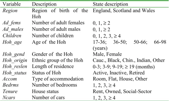
In order to show the potential usefulness of our methodology, we selected thirteen variables describing the British households in terms of composition (variables Ad_fems, Ad_males, Children,
Hoh_age, Hoh_gend), regions of the United Kingdom (variable Region), one ethnicity indicator
(variable Hoh_origin), one mobility indicator (variable Hoh_reslen) and economic indicators of the household (variables Accom, Bedrms, Ncars, Hoh_status, Tenure). A complete description of these
variables and their states are summarized in Table 1. This group of variables was fully observed in the data set extracted from the survey.
The modeling of the data was carried out with the program Bayesware Discoverer, which implements the model search approach described in the previous section.
Variable Description State description
Region Region of birth of the
Hoh
England, Scotland and Wales
Ad_fems Number of adult females 0, 1, ≥ 2
Ad_males Number of adult males 0, 1, ≥ 2
Children Number of children 0, 1, 2, 3, ≥ 4
Hoh_age Age of the Hoh 17-36; 36-50; 50-66; 66-98
(years)
Hoh_gend Gender of the Hoh Male, Female
Hoh_origin Ethnic group of the Hoh Cauc., Black, Chin., Indian, Other
Hoh_reslen Length of residence 0-3; 3-9; 9-19; ≥ 19 (months)
Hoh_status Status of Hoh Active, Inactive, Retired
Accom Type of accommodation Room, Flat, House, Other
Bedrms Number of bedrooms 1, 2, 3, ≥ 4
Tenure House status Rent, Owned, Social-Sector
Ncars Number of cars 1, 2, 3, ≥ 4
Table 1. Description of the variables extracted from the 1996 General Household Survey. Hoh denotes the Head of the Household. Numbers of adult males, females and children refer to the household.
The approach to model selection described in the previous section requires the variables to be discrete. Therefore, the first step of the analysis was to discretize the continuous variables into four bins of approximately equal proportions. Before this step, variables having a skewed distribution were transformed in a logarithmic scale. Many integer-valued variables --- as those indicating the number adult males or females in the household --- were appropriately recoded and states observed with low frequency were grouped into a unique state. We then choose the following order among the variables to limit the space of models to be explored.
Region f Hoh_origin f Hoh_gend f Ad_fems f Ad_mal f Hoh_age f
Hoh_status fChildren f Tenure f Hoh_reslen f Accomod f Bedrms f Ncars.
The choice was based on the following considerations. Geographic variables precede household variables and thus we are interested in conditioning on them first (e.g., see Thomas, et al., 1988). The ordering of some of the household demographic variables (e.g., Hoh_origin, Hoh_gend,
Ad_fems, Ad_males, Hoh_age) and we chose the particular ordering for convenience. These
variables are commonly thought of as explaining house wealth which is described by the variables
Hoh_status, Children, Tenure, Hoh_reslen, Accomod, Bedrms, Ncars, while dependencies in which
interesting. The remaining order was chosen in a similar way, on the basis of possible cause-effect relationships between the remaining variables.
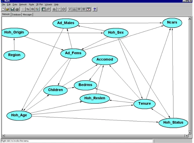
We used this order to build 4 models, using the K2 algorithm, uniform prior probabilities on the possible networks, and symmetric Hyper-Dirichlet prior distributions for the model parameters. We chose four values for the global precision α =1, 5, 10, 20 to evaluate the effect of changing the global prior precision on the model selected. The evaluation was carried out by comparing the networks topologies, and their different predictive capabilities. This last aspect was evaluated by computing the classification accuracy of the four networks. Full details of the analysis are in Sebastiani and Ramoni, (see Sebastiani and Ramoni, 2001) and led to select the network learned with α =5. This network is depicted in Figure 1 and is described in the next section.
Figure 1 The Bayesian network selected from the data when the global prior precision α is 5.
4. Results and discussion
The network in Figure 1 shows important, directed dependencies and conditional independencies. The dependency of the ethnic group of heads of the households on the variable Region reveals a more cosmopolitan society in England than Wales and Scotland, with a larger proportion of Blacks and Indians as head of households. The variables describing the ethnic group of the head of the
household, of the gender of the head of the household, and the number of adult females in the household, separate Region from most of variables describing household wealth.
The working status of the head of the household (variable Hoh_status) is independent of the ethnic group given the gender and age of the head of the household. The estimated conditional probability table shows that when a young female is head of a household, she is much more likely to be inactive than a young male (40% compared to 6% when the age group is 17--36). This difference attenuates as the age of the head of the household increases. The conditional distribution quantifying the dependency of the gender of the head of the household on the ethnic group reveals that Blacks have the smallest probability of having a male head of the household (64%) while Indians have the largest probability (89%).
The age of the head of the household depends directly on the number of adult males and females, and shows that households with no females and two or more males are more likely to be headed by a young male while, on the other hand, households with no males and two or more females are headed by a mid age female. There appear to be more single households headed by an elder female than an elder male. Furthermore, the composition of the household changes in the ethnic groups: the most interesting fact is that Indians have the smallest probability of living in a household with no adult males (10%), while Blacks have the largest probability (32%).
The tenure status of the accommodation depends directly on the age, gender and status of the household head. On the average, the largest proportion of British households is established in owned accommodations (75%), when the age of the head of the household is between 36 and 66 years. Younger heads of household have a larger chance of living in rented accommodations (20%), while senior heads of household have a larger chance of living in accommodations provided by the social service (32%). These figures however change dramatically when the gender of the head of the household is taken into account. When the head of the household is a young female, the probability that the household is in an owned accommodation is 27%, against 65% when the household head is a young male. This probability rises up to 52% when the household head is an elder female compared to 69% for elder males. Households are more likely to be in an accommodation provided by the social service when the head is an inactive female rather than an inactive male.
The number of bedrooms is directly affected by the number of children in the household, the type of accommodation and its tenure status. Households with two or more children are more likely to be in three bedroom flats or houses, but the accommodations provided by the social service are slightly smaller than those rented or owned by the head of the household. Houses are more likely to have a larger number of bedrooms than flats: the most likely number of bedrooms of an owned house is three, compared to one in a flat. Interestingly, flats provided by the social sector are more likely to be one-bed flats, while rented and owned flats are most likely to be two-beds flats. The length of residence is directly dependent on the age of the head of the household and the tenure status of the accommodation and shows that the length of residence in rented accommodations or those provided by the social service is shorter than that in owned accommodations.
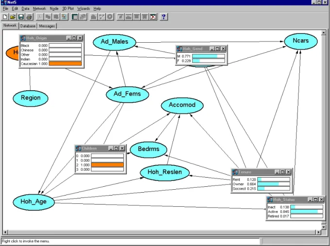
Figure 2 An example of query with the Bayesian network induced from the data.
By querying the network, one may investigate other undirected associations and discover that, for example, the typical Caucasian mid family with two children has 77% chances of being headed by a male who, with probability .57, is aged between 36 and 50 years. The probability that the head of the household is active is .84, and the probability that the household is in an owned house is .66. Results of these queries are displayed in Figure 2.
These figures are slightly different if the head of the household is, for example, Black. In this case, the probability that the head of the household is male (given that there are two children in the household) is only .62 and the probability that he is active is .79. If the head of the household is Indian, then the probability that he is male is .90 and the probability that he is active is .88. On the average, the ethnic group changes slightly the probability of the household being in an accommodation provided by the social service (26% for Blacks, 23% for Chinese, 20% Indians and 24% Caucasians). Similarly, black heads of household are more likely to be inactive than heads of household from different ethnic groups (16% Blacks, 10% Indians, 14% Caucasians and Chinese), and to be living in a less wealthy household, as shown by the larger probability of living in accommodations with a smaller number of bedrooms and of having a smaller number of cars. Households headed by Blacks are less affluent than others, if the gender of the head of the household is not taken into account. However, the dependency structure shows that the gender of the head of the household and the number of adult females make all the other variables independent of the ethnic group. Thus, the model extracted suggests that differences in the household wealth are
more likely caused by the different household composition, and in particular by the gender of the head of the household, rather than racial issues.
The robustness of many of these interpretations can be examined by careful alteration of the ordering of the variables and the structuring of the greedy search algorithm.
5. Conclusions
In this analysis, we focused on networks learned by using uniform model priors and sets of independent, symmetric Dirichlet distributions as prior distribution for each model parameters. The advantage of using these prior distributions is that they can be elicited simply by assigning the global prior precision and this choice produces consistent model comparisons. However, symmetric Dirichlet distributions are known to be too invariant, (see Forster and Smith, 1998), so that they model different dependency structures in the same way. One may wish to use a class of model parameter priors which encodes different prior information. An interesting challenge is to devise a class of prior distributions which maintains the consistency of model comparisons, feasibility of computations, and provides the user with more modeling freedom.
The analysis here was carried out by discretizing all continuous variables, thus raising the issue of the effect of the discretization. We are currently working on the implementation of a more general learning algorithm, which selects networks from data sets with both continuous and discrete variables.
One further issue is related to the publications of the results found with the method described here. A Bayesian network is not just the directed acyclic graph displaying the dependency structure selected, conditional on the data. It is also a probability distribution, and as such, the best way to publish the results is to give the entire network, and to let users make their own queries. Given the increasing importance that the World Wide Web is assuming nowadays as a communication system, publication of the network over the WWW offers a simple way to display results without giving direct access to the original data, thus preserving data confidentiality.
7. Acknowledgements
This research was supported by Eurostat, under contract EP29105. Material from the General Household Survey 1996 is Crown Copyright and has been made available by the Office for National Statistics through The Data Archive and has been used by permission. Neither the ONS nor The Data Archive bear any responsibility for the analysis or interpretation of the data reported here.
6. References
Castillo, E., Gutierrez, J. M., and Hadi, A. S. (1997), Expert Systems and Probabilistic Network
Models, Springer, New York, NY.
Cooper, G. F., and Herskovitz, E. (1992), ‘A Bayesian method for the induction of probabilistic networks from data’, Machine Learning, Vol. 9, pp. 309-347.
Cowell, R. G., Dawid, A. P., Lauritzen, S. L., and Spiegelhalter, D. J. (1999), Probabilistic
Networks and Expert Systems, Springer, New York, NY.
Forster, J. J., and Smith, P. W. F. (1998), ‘Model-based inference for categorical survey data subject to non-ignorable non-response (with discussion)’, Journal of the Royal Statistical Society, B, Vol. 60, pp. 57-70.
Heckerman, D., Geiger, D., and Chickering, D. M. (1995), ‘Learning Bayesian networks: the combinations of knowledge and statistical data’, Machine Learning, Vol. 20, pp. 97-243.
Lauritzen, S. L. (1996), Graphical Models, Oxford University Press, Oxford, UK.
Sebastiani, P., and Ramoni, M. (2001), ‘Data analysis with Bayesian networks’, Under revision. Sebastiani, P., Ramoni, M., and Crea, A. (2000), ‘Profiling customers from in-house data’, ACM
SIGKDD Explorations, Vol. 1, pp. 91-96.
Thomas, M., Walker, A., Wilmot, A., and Bennet, N. (1998), Living in Britain: Results from the