A COMPARISON OF NON-PRICE TERMS OF LENDING
FOR SMALL BUSINESS AND FARM LOANS
Raymond Posey, Mount Union College
Alan K. Reichert, Cleveland State University
ABSTRACT
This study examines differences in terms of lending for small loans among non-farm commercial banks and farm lenders of different sizes. Large farm lenders more frequently require collateral than large commercial banks, while small farm lenders require collateral less frequently than small commercial banks. In addition, there is evidence that small commercial banks require collateral more frequently than large commercial banks. There is no difference in the frequency of collateral use among farm lenders, regardless of size. The type of the collateral used, real estate vs. non-real estate, is also affected by the term of the loan for farm lenders. The longer the term of the loan, the more frequently real estate is used as collateral.
JEL: G2
KEYWORDS: farm lending, role of collateral, terms of lending INTRODUCTION
anks set lending terms in a negotiation with borrowers in an effort to earn a target rate of return and manage the probability of default (PD) and loss given default (LGD). Varying interest rates and non-price terms, such as collateral, can reduce the LGD. However, Stiglitz and Weiss (1981) show that raising interest rates and increasing collateral requirements above a maximum amount can actually reduce the expected return to the bank. This occurs because of adverse selection, in which case only the riskiest borrowers will accept the higher interest rates. Because of this behavior, lenders would have more risk than the higher interest rates compensate for, explaining the lower returns to the lender as interest rates increase. Given this situation, it is rational for banks to ration credit (refuse to lend to certain borrowers), rather than attempt to price it with higher interest rates. This explains why total lending volume may decline in response to tightened lending standards.
Small borrowers tend to be more informationally opaque than large, publicly traded firms. There is a large body of research that examines bank relationship lending by banks. In this case, the banks place some reliance upon the prior relationship with a borrower and the knowledge gained from that relationship, such as cash flows observed in checking accounts. Both loans to the small non-farm (commercial) business sector and loans to the small farm sector represent different forms of small business lending. Given the substantial differences in the risk these firms face and the types of assets such firms possess, it is possible that lenders to these two sectors may view collateral in significantly different ways. This may especially be true since farm businesses are characterized by large fixed assets in the form of land and equipment and are subject to a high degree of output price volatility. The reminder of this paper is organized as follows. Section 2 reviews the prior literature. Section 3 discusses the methodology and the empirical model. Section 4 presents the empirical findings, while Section 5 presents the conclusion.
LITERATURE REVIEW
Many other authors have examined the use of collateral as a non-price means to resolve the asymmetric information between borrower and lender. The borrower knows better than the lender the true risk of the business, and in the case of small businesses, information asymmetry is higher because of the absence of public disclosure of financial data, as is the case with publicly traded companies. Boot and Thakor (1994) examine the use of collateral and conclude that collateral is more likely to be used on a first loan related to a short or non-existent prior banking relationship. The need for collateral can then be reduced or eliminated on subsequent loans to the same borrower following a successful initial loan contract
There are a group of studies that focus on the effects of the lender-borrower relationship on interest rates and the use of collateral. Machauer and Weber (1998) find that German borrowers offer more collateral to their “housebank”, the bank with whom they have a primary banking relationship. In this case, it appears the banks may exploit the relationship or are using their private knowledge of the small firm to set the terms of lending. This seems to suggest that a closer banking relationships lead to greater use of collateral, perhaps because the inside knowledge of the lender enable them to identify collateral which might be available to pledge. Contrary to this finding, Elsas and Krahnen (1999) find an inverse relationship between the use of collateral and the strength of the banking relationship. Brick and Palia (2007) examine the use of collateral, loan interest rates, and the length of lending relationships. Here, the length of the banking relationship is used as a measure of the strength of the relationship. They review prior research noting mixed findings on the inter-relationships among interest rate, collateral, and the length of the banking relationship. Berger and Udell (1990) find a positive relationship between the use of collateral and interest rates, whereas in a later study, Berger and Udell (1990) find a no relationship. Chakraborty and Hu (2006) examine the use of collateral in small business loans. They examine multiple types of loans, including lines of credit and others types, such as fixed term loans. They find a negative relationship between the length of the bank-borrower relationship and the use of collateral for lines of credit. The relationship length is not significant for other types of loans. One key difference between the research of Brick and Palia (2007) versus Chakraborty and Hu (2006) is whether the terms of lending are endogenous or exogenous. Brick and Palia (2007) argue that they are endogenous and use a two-stage procedure in their econometric analysis. This same method is employed in Essay #1 for the same reason. Both Essay #1 and Brick and Palia (2007) find evidence that key loan terms are in fact determined jointly, or simultaneously, and therefore those variables are not predetermined but rather are endogenous. Overall, there is mixed evidence with regard to the relationship between length of the bank lending relationship and the use of collateral. There is also mixed empirical evidence regarding the interplay between the use of collateral and other lending terms.
Walraven and Barry (2004), using data from the Survey of Terms of Bank Lending to Farmers and from call reports, examine the relationship between the effective interest rate charged and various price and non-price terms of lending. They find that secured loans (using collateral) have a higher effective interest rate as do loans secured by farm real estate. In this case, collateral appears to be a complement to interest rates, rather than being a substitute. An important difference in loans to small businesses and loan to farms is that according to Walraven and Barry (2004), over 60% of farm loans are made by small commercial banks. In contrast, approximately 43% of small non-farm commercial loans (<$100,000) are made by small commercial banks based on the November, 2008 Federal Reserve’s Terms of Business Lending survey. Thus, not only are the two borrowing sectors, farm and non-farm, unique their primary lenders are quite different as well. Lown and Morgan (2006) examine the effects of changes in loans standards on the quantity of loans made. They argue that the loan standards variable (taken from the Loan Officer Opinion Survey) is an approximate index for a vector of non-price lending terms. They show, using a VAR model, that the volume of C&I loans (commercial and industrial) is negatively effected by an increase in lending standards.
DATA AND METHODOLOGY Hypotheses
As discussed above, collateral is a common feature of bank loans that can reduce both the probability-of-default (PD) and the loss- given-probability-of-default (LGD) to the lender and attempt to control asymmetric information between lender and borrower. The empirical evidence regarding the role of collateral is mixed. Given the previous mixed empirical findings, the following broad questions will be addressed in this study: 1) What are the differences in the terms of lending between small business commercial loans and similar (non-real estate) loans to farmers, and how do these differences vary over time?, 2) How are loan risk, collateral, and interest rates related for these two different types of farms and non-farm borrowers?, and 3) How are these lending term relationships affected by the size of the lender?
Farms typically are fixed-asset intensive because both land and equipment is required. As a result, it is anticipated that lenders will seek to use the more readily available and easy to identify collateral for non-real estate loans to farmers. There is evidence from Chakraborty & Hu (2006) that more collateral is required as the size of the borrower (total assets) increases. Furthermore, small banks typically lend to local and regional small borrowers, which may be concentrated by industry type. This would tend to concentrate credit risk in smaller banks where it is more difficult to diversify their loan portfolio. For example, smaller rural banks located in agricultural areas are like to have a loan portfolio heavily concentrated in farm loans to local borrowers. Therefore, the following three hypotheses are tested: H1: Collateral will be more prevalent in farm lending than in small non-farm commercial loans
H2: Small banks require more collateral than larger lenders due to their more concentrated higher risk loan portfolios.
H3: The importance of collateral will change over time as lenders modify their underwriting (credit) standards to reflect changes in external economic conditions and their internal risk management strategies.
Data
The Federal Reserve Board conducts two quarterly surveys of the terms of lending, one for business (C&I) lending, and one for lending to farmers. More formally, the business lending survey is named E.2 Survey of Terms of Business Lending (STBL), and the other is named E.15 Agricultural Finance Databook (AFD). Both surveys are quarterly and since 1999Q4 have provided the same information with regard to summary loan data. The AFD has more variables and more detailed information than is provided in the STBL, and in some cases has more years of data. It is subdivided into three sections; A) Amount and Characteristics of Farm Loans Made by Commercial Banks; B) Selected Statistics from the Quarterly Reports of Condition of Commercial Banks; and C) Reserve Bank Surveys of Farm Credit Conditions and Farm Land Values.
For this study, the data period is from 2002(Q2) – 2009(Q1). The following six variables common to both surveys will be used: 1) percentage of loans secured by collateral, 2) effective interest rate, 3) degree of credit risk, 4) dollar volume of loans, 5) weighted average maturity, and 6) percentage of loans made under commitment. Both farm and non-farm surveys are subdivided into small and large bank (lenders) categories, so comparisons of the effects of bank size can be made by comparing the results of the same model for the two different size categories. Likewise, comparisons between farm lending and C&I lending can be made using identical models with the different data sets. Loans up to $99,000 are included in this study. One additional variable from the Senior Loan Officer Opinion Survey is used. It is the net
percentage of domestic bank respondents that are tightening standards. (That is, the percent of banks that have tightening their credit standards less the percentage of banks that have loosened their lending standards). There are two standards time series, one for small borrowers and one for large. While the size of the typical borrower is not known, since this study examines loans smaller than $100K, it is presumed that the standards series for small borrowers would be most appropriate. Regardless, as shown by Lown and Morgan (2006) the two series are highly correlated. For these time series, the two series have a Pearson correlation coefficient of .968, which is significant at the 1% level. For this study, the small borrower lending standards series will be used.
Although the time series is relatively short (38 quarters), this data does offer the opportunity for examining effects of changes of lending terms on subsequent borrower behavior. All of the time series were tested for the presence of unit roots using the augmented Dickey Fuller procedure. For the variables where the null hypothesis of a unit root cannot be rejected (5% level of significance), they are included in the model in first difference form. When this is the case, either the first or second letter of the variable name is a “D”, indicating it is a differenced variable. Furthermore, if the first letter in a variable name is “F”, this indicates that the variable applies to a farm lender. If the last letter is an “L”, the variable applies to a large lender.
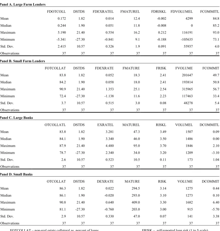
In Table 1, descriptive statistics of the AFD and STBL for the entire time series are provided for the common variables. The data is provided for large farm banks, small farm banks, and for small and large banks. The variables are defined as follows:
1) FOTCOLLAT – non-real estate collateral as a percent of total loans. 2) DSTD – net percentage of lenders increasing lending standards.
3) FDEXRATE – weighted average effective interest rate of loans in excess of the comparable maturity treasury rate.
4) FRISK – weighted average loan risk rating on a scale from 1 to 5, with 5 being the highest risk. The risk ratings are assigned by the lender.
5) FDVOLUME – volume (size) of lenders total loan portfolio ($billions) 6) FMATURE – weighted average maturity of the loan portfolio in months
7) FCOMMIT – percentage of loans made under a prior loan commitment
One difference between the variables in the two surveys is the presence of two collateral variables in the AFD data. The value of the non-real estate collateral (“other” collateral) variable (OTCOLLAT) is the percentage of loans that have non-real estate collateral. Even though the loans examined in this study are non-real estate loans, a portion of the collateral actually used to support non-real estate lending is based on real estate. Given the nature of farms, it is not surprising that collateral of this type may be used for non-real estate loans. A preliminary evaluation of these two forms of collateral reveals that they are negatively correlated. This suggests subsequent analysis must use a single collateral variable due to a high degree of multi-collinearity It also suggests that total collateral variable which is the sum of real estate collateral (RECollat) and non-real estate collateral (OtCollat) may mask differing relationships. The correlation between the two variables is -0.87.
Machauer and Weber (1998) discuss the presence of “money illusion”, which is the tendency for interest rate risk premiums, measured over some risk free rate, to be lower when nominal interest rates are high and higher when nominal rates are low. To borrowers this procedure appears to stabilize their borrowing rates over the interest rate cycle. There is evidence of this rate smoothing phenomenon over the sample period as the correlation between the fed funds rate and the borrowers risk premium (Exrate) is -0.74.
Table 1 - Descriptive Statistics Panel A. Large Farm Lenders
FDOTCOLL DSTDS FDEXRATEL FMATUREL FDRISKL FDVOLUMEL FCOMMITL
Mean 0.172 1.82 0.014 12.4 -0.002 4299 84.8 Median 0.244 1.90 0.051 11.8 -0.008 0 85.2 Maximum 5.190 21.40 0.554 16.2 0.212 116191 93.0 Minimum -5.341 -27.30 -0.841 9.1 -0.188 -105635 73.1 Std. Dev. 2.415 10.57 0.326 1.9 0.091 55937 4.0 Observations 37 37 37 37 37 37 37
Panel B. Small Farm Lenders
FOTCOLLAT DSTDS FDEXRATE FMATURE FRISK FVOLUME FCOMMIT
Mean 83.8 1.82 0.052 18.3 2.41 201647 49.7 Median 84.2 1.90 0.058 18.0 2.41 193814 50.8 Maximum 90.9 21.40 1.353 25.1 2.54 315965 56.7 Minimum 72.4 -27.30 -1.138 11.6 2.23 117463 33.4 Std. Dev. 3.7 10.57 0.515 3.0 0.08 48278 5.4 Observations 37 37 37 37 37 37 37
Panel C. Large Banks
OTCOLLATL DSTDS EXRATEL MATUREL RISKL VOLUMEL DCOMMITL
Mean 83.8 1.82 3.281 47.3 3.49 1507 0.09 Median 84.1 1.90 3.340 46.0 3.50 1486 0.00 Maximum 87.9 21.40 4.480 95.0 3.70 1846 2.10 Minimum 78.7 -27.30 2.340 34.0 3.20 1209 -3.10 Std. Dev. 2.6 10.57 0.523 10.5 0.11 173 1.04 Observations 37 37 37 37 37 37 37
Panel D. Small Banks
OTCOLLAT DSTDS DEXRATE MATURE RISK VOLUME DCOMMIT
Mean 86.3 1.82 0.022 294.5 3.14 1275 0.44 Median 86.1 1.90 -0.020 293.0 3.10 1273 0.10 Maximum 90.8 21.40 0.640 409.0 3.30 1682 6.40 Minimum 81.1 -27.30 -0.760 203.0 3.00 915 -5.70 Std. Dev. 2.9 10.57 0.330 47.0 0.07 141 3.38 Observations 37 37 37 37 37 37 37
FOTCOLLAT – non-real estate collateral as percent of loans. FRISK – self-reported loan risk (1 to 5 scale)
DSTD – percentage of lenders increasing lending standards. FDVOLUME – loan volume (millions of dollars)
FDEXRATE – interest rate of loans in excess of an appropriate treasury rate. FMATURE – The maturity of the loans (months) FCOMMIT – The percentage of loans made under prior commitment
Alternative Models
The first model to be estimated will be of the following contemporaneous OLS regression: COLLATERALt= α + β1STANDARDSt+ β2EXRATEt+ β3MATURE + β4RISKt+ β5VOLUMEt+
β6COMMIT + εt (1)
This OLS equation will be estimated for four categories of lenders: large and small commercial banks and large and small farm lenders. The presence of possible non-stationarity in the data will be examined and corrected as necessary. Furthermore, Newey-West robust coefficients will be used to address the presence of autocorrelation or heteroscedasticity. Depending upon empirical findings, it may be appropriate to include a lag of the STANDARDS variable rather than its contemporaneous value.
In order to capture dynamic time-varying inter-relationships effects among the variables a vector auto-regressive (VAR) model will be estimated similar to the model used by Lown and Morgan (2004). As discussed previously, certain prior studies consider terms of lending to be exogenous, whereas other research considers the terms of lending to be endogenous or jointly determined. The VAR procedure is quite flexible since it assumes that all the variables in the model are potentially interrelated or endogenous. The VAR model will include the same variables as shown in equation (1) except that the right hand side will include lags of both the dependent variable and selected independent variables. Thus, the VAR model is a series of equations, all of the form specified in equation (2), where the number of equations is equal to the number of variables. To illustrate, the general form of the VAR model will be as follows:
COLLATERALt= β0+ Σβ1iSTANDARDSt-i+ Σβ2iEXRATEt-i+ Σβ3iMATUREt-i+ Σβ4iRISKt-i+
Σβ5iVOLUMEt-i+ Σβ6iCOMMITt-i + Σβ7iCOLLATERALt-i + εt (2)
where, Σ indicates the inclusion of lags of the variables from time t-1 to time n. The number of lags (n) to be used is an empirical matter and will be based on the lowest values for the AIC and SIC summary statistics. The number of lags of the variables will be limited because of the relatively short length of the time series. Given the limited number of degrees of freedom, the VAR model will be estimated using only those independent variables found to be statistically significant in equation (1). The credit standards variable may or may not be exogeneous. Loan and Morgan (2006) suggest that it represents a proxy for all non-price terms of lending. In their research, they find a negative relationship between credit standards and aggregate loan volume and assume credit standards to be exogenous. However, it may be that lenders, in order to properly manage their loan portfolio, may adjust underwriting standards for internal purposes, and not simply in response to external economic factors or monetary policy changes.
Finally given the expectation that tightening of lending standards will influence both priced and non-price terms of lending, Granger causality tests will be conducted to determine which variable(s) appear to precede or “cause” the others variables to change. While the appropriate number of lags is an empirical matter, prior research suggests that no more than 4 lags should be necessary.
EMPIRICAL RESULTS OLS Results
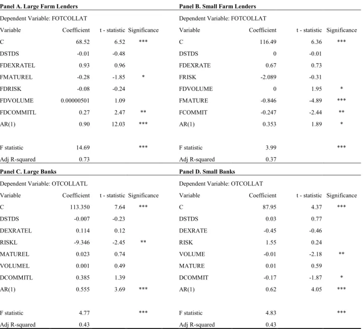
Equation (1) was first estimated using OLS for the four categories of lenders. These results are provided in Table 2, Panels A-D. Six variables are used in each model. The credit standards variable used in each model is specified in first difference form (DSTD), hence a positive value for the variable would indicate that credit standards are being tightened at an increasing rate. Several other independent variables, loan
commitment (COMMMITL), interest rate risk premium (DEXRATEL), and loan volume (VOLUME) are also specified in first difference form as needed to correct for non-stationarity.
The dependent variable in this section is specified in levels, not in first difference form. The model for Large Farm Lenders (Panel A) showed strong first-order auto-correlation, while the Durbin-Watson statistic for the other models was marginal at the 5% level. Thus, all four models include a first-order autoregressive term, AR(1), which proved to be highly significant in all models. In addition, all models were tested for the presence of heteroscedasticity, using both the White and Bruesch-Pagan-Godfrey tests. In Panel A, the results for Large Farm Lenders are provided. FMATURITY is significant at the 10% level and carries a negative sign. This result is consistent with the previously mentioned correlation where maturity is negatively correlated with use of non-real estate collateral. FCOMMITL is positive and significant at the 5% level. The credit standards variable is not significant.
The equation estimated in Panel B for small farm loans is significant at the 1% level, but once again the standards variable is not significant. As with large lenders, loan maturity (FMATURE) is negative and statistically significant. Risk is not significant. Maturity is negative and significant, as is the case for large farm lenders. Loan volume is positive and significant, while the coefficient on loan commitment (FCOMMIT) is negative and significant at the 5% level. The interest rate variables, FRISK and FEXRATE, are not statistically significant.
The OLS results for large commercial banks are provided Panel C. The overall regression is significant at the 1% level and loan risk (RISKL) is the only significant variable in the model and carries a negative coefficient. This sign may appear inconsistent with expectations as it would be expected that banks would require collateral on riskier loans to mitigate the risk. An alternate explanation for the negative sign is that the loan portfolio is riskier because fewer loans require collateral. This could occur when the competitive environment forces banks to reduce their collateral demands in order to secure the loan. In Panel D., the results for small commercial banks are provided. Loan volume is significant and negatively related to collateral usage. This negative relationship between loan volume contrasts to the positive but small coefficient reported in Panel B. This may be due to abundant levels of both real estate and non-real estate collateral available from farms borrowers. Loan commitment (DCOMMIT) is also significant at the 10% and negatively related to collateral usage.
To summarize the OLS results, in the regression for large farm lenders, maturity and commitment are significant at conventional levels. Maturity is also negative and significant for small farm lenders. Commitment is significant, but negatively related to collateral, contrary to the findings for large farm lenders. For small farm lenders, the first difference of volume is used in the analysis so the proportion of collateral used increases as volume increases. Risk is the only significant variable for large banks. For small banks, higher volume is associated with a lower proportion of collateral in loans, suggesting looser terms of lending in periods of higher volume. For both types of small lenders, the proportion of loans made under commitment is negatively associated with the proportion of collateral required, suggesting borrowers may benefit from the prior commitment regarding collateral requirements when compared to current lending standards. For small farm lenders, loan maturity is negative and significant, consistent with the finding that non-real estate collateral is negatively related to loan term. The most consistent finding is that commitment is significant in three of the four lender type estimations. In general, each lender category appears to have unique, contemporaneous explanatory variables for the proportion of loans requiring collateral.
Table 2 - OLS Regression Results
Panel A. Large Farm Lenders Panel B. Small Farm Lenders
Dependent Variable: FOTCOLLAT Dependent Variable: FOTCOLLAT
Variable Coefficient t - statistic Significance Variable Coefficient t - statistic Significance
C 68.52 6.52 *** C 116.49 6.36 *** DSTDS -0.01 -0.48 DSTDS 0 -0.01 FDEXRATEL 0.93 0.96 FDEXRATE 0.67 0.73 FMATUREL -0.28 -1.85 * FRISK -2.089 -0.31 FDRISK -0.08 -0.24 FDVOLUME 0 1.95 * FDVOLUME 0.00000501 1.09 FMATURE -0.846 -4.89 *** FDCOMMITL 0.27 2.47 ** FCOMMIT -0.247 -2.44 ** AR(1) 0.90 12.03 *** AR(1) 0.353 1.89 * F statistic 14.69 *** F statistic 3.99 ***
Adj R-squared 0.73 Adj R-squared 0.37
Panel C. Large Banks Panel D. Small Banks
Dependent Variable: OTCOLLATL Dependent Variable: OTCOLLAT
Variable Coefficient t - statistic Significance Variable Coefficient t - statistic Significance
C 113.350 7.64 *** C 87.95 4.37 *** DSTDS -0.007 -0.23 DSTDS 0.03 0.77 DEXRATEL 0.114 0.12 DEXRATE -0.45 -0.46 RISKL -9.346 -2.45 ** RISK 1.55 0.24 MATUREL 0.023 0.74 VOLUME -0.01 -2.18 ** VOLUMEL 0.001 0.49 MATURE 0.01 0.59 DCOMMITL 0.385 1.39 DCOMMIT -0.17 -1.87 * AR(1) 0.555 3.69 *** AR(1) 0.62 4.05 *** F statistic 4.77 *** F statistic 4.83 ***
Adj R-squared 0.43 Adj R-squared 0.43
This table presents the OLS results for each of the four lender types. The equation estimated is of the form:
COLLATERALt = α + β1STANDARDSt + β2EXRATEt + β3MATURE + β4RISKt + β5VOLUMEt + β6COMMIT + εt
The data is from the period 2002Q2 - 2009Q1. ***, **, * denotes significance at the 1%, 5%, and 10% level, respectively. VAR Results
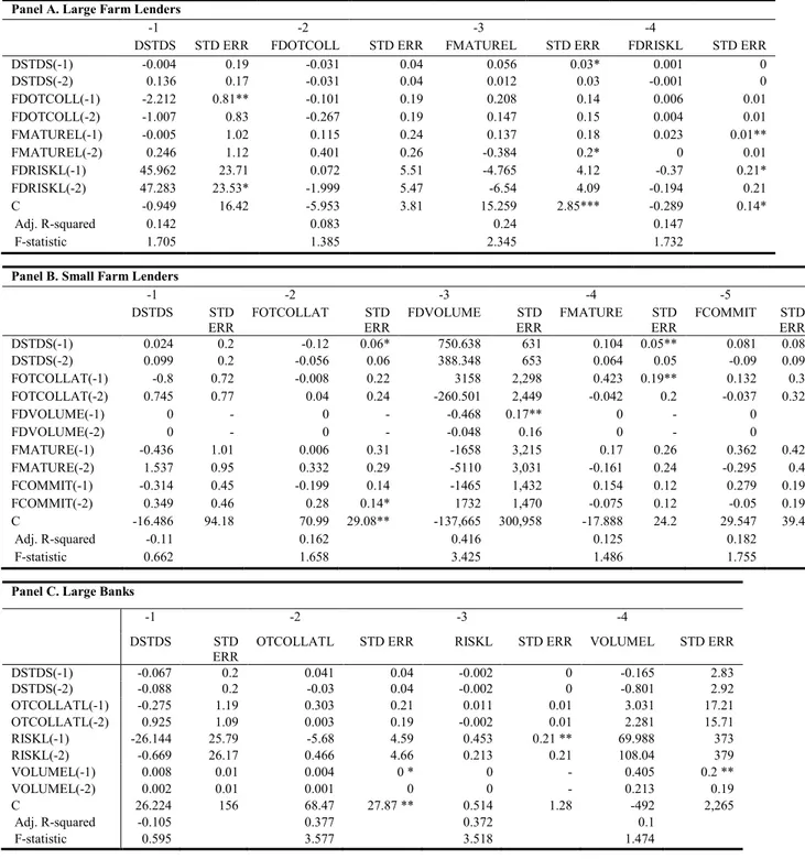
VAR models of the form described in equation (2) were estimated for each of the four lender categories and the results are provided in Table 3, Panels A-D. Because of the limited number of observations, all the VAR models include the collateral and standards variables, and at least two more variables having the lowest p value in their respective OLS regression. Furthermore, all variables with significance levels below 0.10 are included in the respective VAR model.
The VAR results for large farm lenders are provided in Panel A. In equation (1) DSTD are explained by one lag of FDOTCOLL and one and two lags of FDRISKL. Thus, as collateral is increased lending standards are subsequently loosened, and as loan risk increases credit standards are subsequently
tightened. In equation (2) none of lagged variables appear to impact FDOTCOLL in a significant way. The strongest explanatory variable identified in equation (3) for FMATUREL is its own value lagged two quarters. One lag of DSTD is also significant, suggesting that maturities increase in response to tightening standards. In equation (4) the variable FMATUREL lagged one quarter has a positive impact on changes in loan risk (FDRISKL). This suggests that as maturity increases, loan risk subsequently increases.
The results for small farm loans reported in Panel B in equation (1) for DSTD indicate that none of the explanatory variables are significant. In equation (2), FOTCOLLAT is explained by one lag of DSTD (negative sign) and two lags of FCOMMIT, which is positive and statistically significant. In equation (3) FDVOLUME is explained by a one quarter lag in its own value which carries a negative coefficient. Thus, an increase in loan volume is followed by a subsequent decrease in volume. In equation (4), FMATURE is explained by one lag of DSTD and one lag of FOTCOLLAT, both with positive coefficients. This suggests that as standards tighten and collateral is required more, loan maturities increase. In equation (5), FCOMMIT is explained by both one and two lags of FDVOLUME, where the signs of both coefficients are both positive. This indicates that as volume increases, the proportion of loans made under commitment increases in subsequent quarters.
The results for large commercial banks are provided in Panel C. None of the lags of the variables are significant in explaining the DSTD in equation (1). One lag of VOLUMEL is positive and significant in explaining OTCOLLAT in equation (2). As previously noted, VOLUMEL was not significant at conventional levels in the contemporaneously OLS model, but one lag is significant here, suggesting that loan volume increases lead to increased use of collateral in the following quarter. In equation (3) loan RISK is positively related to its own value lagged one period and the same is true for loan volume in equation (4).
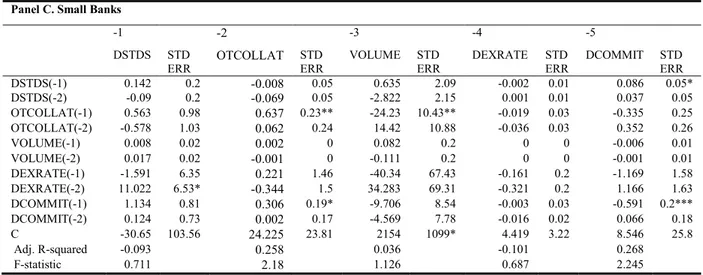
The VAR results for small commercial banks are provided in Panel D. In equation (1) the value of the risk premium lagged two quarters is weakly related to changes in loan standards two quarters later. In equation (2) the one quarter lagged value of OTCOLLAT is positively related to OTCOLLAT. In equation (3) one lag of OTCOLLAT is negative and significant in explaining VOLUME. This result is similar to the findings for small farm lenders where one lag of FOTCOLLAT is positive and significant in the FDVOLUME equation. None of the lagged variables are significant in explaining risk premiums (DEXRATE) as indicated in equation (4), indicating once again that contemporaneous relationships may be more important. However, one lag of DSTD is significant in the DCOMMIT model, equation (5), suggesting that as lending standards tighten more loans are made under commitment. Perhaps this occurs because borrowers take advantage of the pre-existing loan commitment to obtain new loans after standards are tightened. Finally, as seen in equation (5) the percent of loan commitments is negatively related to its lagged value.
Granger Causality
Given the complex lag relationships between the variables as evidenced by the VAR analysis, Granger causality is explored. Table 4 - Panels A-D provides the Granger results for each of the four loan samples. Lags of 5 or more quarters were not found to be significance. In many cases, two lags were sufficient to demonstrate a relationship. For all analyses in this section, 4 quarterly lags are used. While analyses were conducted among all pairs of variables in the model, only the results indicating Granger causality at the 10% level or better are reported in Table 4.
Table 3 - VAR Results Panel A. Large Farm Lenders
-1 -2 -3 -4
DSTDS STD ERR FDOTCOLL STD ERR FMATUREL STD ERR FDRISKL STD ERR
DSTDS(-1) -0.004 0.19 -0.031 0.04 0.056 0.03* 0.001 0 DSTDS(-2) 0.136 0.17 -0.031 0.04 0.012 0.03 -0.001 0 FDOTCOLL(-1) -2.212 0.81** -0.101 0.19 0.208 0.14 0.006 0.01 FDOTCOLL(-2) -1.007 0.83 -0.267 0.19 0.147 0.15 0.004 0.01 FMATUREL(-1) -0.005 1.02 0.115 0.24 0.137 0.18 0.023 0.01** FMATUREL(-2) 0.246 1.12 0.401 0.26 -0.384 0.2* 0 0.01 FDRISKL(-1) 45.962 23.71 0.072 5.51 -4.765 4.12 -0.37 0.21* FDRISKL(-2) 47.283 23.53* -1.999 5.47 -6.54 4.09 -0.194 0.21 C -0.949 16.42 -5.953 3.81 15.259 2.85*** -0.289 0.14* Adj. R-squared 0.142 0.083 0.24 0.147 F-statistic 1.705 1.385 2.345 1.732
Panel B. Small Farm Lenders
-1 -2 -3 -4 -5
DSTDS STD
ERR FOTCOLLAT ERR STD FDVOLUME ERR STD FMATURE ERR STD FCOMMIT ERR STD
DSTDS(-1) 0.024 0.2 -0.12 0.06* 750.638 631 0.104 0.05** 0.081 0.08 DSTDS(-2) 0.099 0.2 -0.056 0.06 388.348 653 0.064 0.05 -0.09 0.09 FOTCOLLAT(-1) -0.8 0.72 -0.008 0.22 3158 2,298 0.423 0.19** 0.132 0.3 FOTCOLLAT(-2) 0.745 0.77 0.04 0.24 -260.501 2,449 -0.042 0.2 -0.037 0.32 FDVOLUME(-1) 0 - 0 - -0.468 0.17** 0 - 0 * FDVOLUME(-2) 0 - 0 - -0.048 0.16 0 - 0 *** FMATURE(-1) -0.436 1.01 0.006 0.31 -1658 3,215 0.17 0.26 0.362 0.42 FMATURE(-2) 1.537 0.95 0.332 0.29 -5110 3,031 -0.161 0.24 -0.295 0.4 FCOMMIT(-1) -0.314 0.45 -0.199 0.14 -1465 1,432 0.154 0.12 0.279 0.19 FCOMMIT(-2) 0.349 0.46 0.28 0.14* 1732 1,470 -0.075 0.12 -0.05 0.19 C -16.486 94.18 70.99 29.08** -137,665 300,958 -17.888 24.2 29.547 39.4 Adj. R-squared -0.11 0.162 0.416 0.125 0.182 F-statistic 0.662 1.658 3.425 1.486 1.755
Panel C. Large Banks
-1 -2 -3 -4
DSTDS STD
ERR OTCOLLATL STD ERR RISKL STD ERR VOLUMEL STD ERR
DSTDS(-1) -0.067 0.2 0.041 0.04 -0.002 0 -0.165 2.83 DSTDS(-2) -0.088 0.2 -0.03 0.04 -0.002 0 -0.801 2.92 OTCOLLATL(-1) -0.275 1.19 0.303 0.21 0.011 0.01 3.031 17.21 OTCOLLATL(-2) 0.925 1.09 0.003 0.19 -0.002 0.01 2.281 15.71 RISKL(-1) -26.144 25.79 -5.68 4.59 0.453 0.21 ** 69.988 373 RISKL(-2) -0.669 26.17 0.466 4.66 0.213 0.21 108.04 379 VOLUMEL(-1) 0.008 0.01 0.004 0 * 0 - 0.405 0.2 ** VOLUMEL(-2) 0.002 0.01 0.001 0 0 - 0.213 0.19 C 26.224 156 68.47 27.87 ** 0.514 1.28 -492 2,265 Adj. R-squared -0.105 0.377 0.372 0.1 F-statistic 0.595 3.577 3.518 1.474
Table 3 - VAR Results Continued Panel C. Small Banks
-1 -2 -3 -4 -5
DSTDS STD
ERR OTCOLLAT STD ERR VOLUME STD ERR DEXRATE STD ERR DCOMMIT STD ERR
DSTDS(-1) 0.142 0.2 -0.008 0.05 0.635 2.09 -0.002 0.01 0.086 0.05* DSTDS(-2) -0.09 0.2 -0.069 0.05 -2.822 2.15 0.001 0.01 0.037 0.05 OTCOLLAT(-1) 0.563 0.98 0.637 0.23** -24.23 10.43** -0.019 0.03 -0.335 0.25 OTCOLLAT(-2) -0.578 1.03 0.062 0.24 14.42 10.88 -0.036 0.03 0.352 0.26 VOLUME(-1) 0.008 0.02 0.002 0 0.082 0.2 0 0 -0.006 0.01 VOLUME(-2) 0.017 0.02 -0.001 0 -0.111 0.2 0 0 -0.001 0.01 DEXRATE(-1) -1.591 6.35 0.221 1.46 -40.34 67.43 -0.161 0.2 -1.169 1.58 DEXRATE(-2) 11.022 6.53* -0.344 1.5 34.283 69.31 -0.321 0.2 1.166 1.63 DCOMMIT(-1) 1.134 0.81 0.306 0.19* -9.706 8.54 -0.003 0.03 -0.591 0.2*** DCOMMIT(-2) 0.124 0.73 0.002 0.17 -4.569 7.78 -0.016 0.02 0.066 0.18 C -30.65 103.56 24.225 23.81 2154 1099* 4.419 3.22 8.546 25.8 Adj. R-squared -0.093 0.258 0.036 -0.101 0.268 F-statistic 0.711 2.18 1.126 0.687 2.245
This table presents the Vector Autor Regression (VAR) results for the two sizes of banks. The equation esimated is of the form:
COLLATERALt = β0 + Σβ1iSTANDARDSt-i + Σβ2iEXRATEt-i + Σβ3iMATUREt-i + Σβ4iRISKt-i + Σβ5iVOLUMEt-i
+ Σβ6iCOMMITt-i + Σβ7iCOLLATERALt-i + εt Two lags are included for each variable. The dependent variable is listed at the top of the
column. The data sample is from 2000Q3 through 2009Q1. The standard error is denoted by STD ERR. ***, **, * denotes significance at the 1%, 5%, and 10% level, respectively
Panel A provides the results for large farm lenders. A number of significant relationships are shown. The use of collateral is Granger caused by maturity, loan commitments, and standards. Loan maturity is Granger caused by both risk and volume. Loan risk is Granger caused by the interest rate risk premium. Credit standards is Granger caused by loan commitments. Panel B provides the results for small farm lenders. The use of collateral is Granger caused by standards and loan commitments and is somewhat similar to the case for large farm lenders, except that maturity is not significant. Maturity is Granger caused by the interest rate premium, loan commitments, and volume. The interest rate premium is Granger caused by standards and loan commitments. Risk and Volume are Granger caused by maturity. Loan commitments are Granger caused by loan volume.
Granger causality appears to be weaker and less prevalent among commercial banks compared to farm lenders. For example for large commercial banks (Panel C), there are a much smaller number of significant relationships. Lending standards Granger causes maturity, while loan commitments Granger cause changes in the interest rate premium, and loan volume Granger causes changes in loan commitments. Finally, Panel D provides the results for small commercial banks. Loan commitments are Granger caused by collateral and credit standards. Collateral Granger causes interest rate premiums and risk Granger causes Standards. For small commercial banks, most of the relationships found are only weakly significant at only the 10% level. Unlike farm lenders, the picture of Granger causality is quite different for banks. For each pair of variables where Granger causality is significant, the pairs differ between large and small banks. The only common causal factor is standards where for large banks it Granger causes maturity and for small banks it Granger causes commitment. Each bank type appears to have its own unique relationship with regard to Granger causality.
Given their close interrelationship, the following briefly summarizes both the VAR and Granger causality results. Loan commitments have a generally consistent effect on the use of collateral among farm lenders. For small farm lenders, loan commitments explains the use of collateral in the OLS regression and in the VAR results, two lags of loan commitment are also significant in explaining collateral usage. Loan commitment is shown to Granger-cause the use of non-real estate collateral for both larger and small farm lenders. These findings support the view that changes in the proportion of loans made under commitments affects the use of collateral. One possible explanation is that as standards tighten,
borrowers may be more inclined to exercise a prior loan commitment rather than requesting a new loan with their current bank or seeking a loan with a new lender. It may also be that under these circumstances, current collateral requirements have become tougher, so it is preferable to the borrower to exercise the prior commitment. Note that in the small farm lender OLS analysis, the coefficient for commitment is negative and significant, which is consistent with this explanation. The use of non-real estate collateral in small lenders, regardless of type, is influenced by contemporaneous changes in lending volume and commitment. The sign on commitment is always negative, indicating that as the proportion of loans made under commit increase, the proportion of loans requiring collateral decreases. However, the sign on volume is positive for small farm lenders but negative for small commercial banks, indicating a lender-specific difference in behavior. Changes in loan credit standards over time play a role in many of the relationships observed.
Table 4: Granger Causality Results Panel A. Large Farm Lenders
Null Hypothesis: Obs. F-statistic Probability
DSTDS does not Granger Cause FDOTCOLL 33 2.212 0.098 *
FMATUREL does not Granger Cause FDOTCOLL 33 4.016 0.012 **
FCOMMITL does not Granger Cause FDOTCOLL 33 3.414 0.024 **
FCOMMITL does not Granger Cause DSTDS 33 2.975 0.040 **
FMATUREL does not Granger Cause FDEXRATEL 33 2.833 0.047 **
FDEXRATEL does not Granger Cause FDRISKL 33 3.571 0.020 **
FDRISKL does not Granger Cause FMATUREL 33 2.900 0.043 **
FDVOLUMEL does not Granger Cause FMATUREL 33 2.472 0.072 *
Panel B. Small Farm Lenders Obs. F-statistic Probability
DSTDS does not Granger Cause FOTCOLLAT 33 4.0612 0.0118 **
FCOMMIT does not Granger Cause FOTCOLLAT 34 3.2831 0.0271 **
DSTDS does not Granger Cause FDEXRATE 33 2.6632 0.0571 *
FDEXRATE does not Granger Cause FMATURE 33 3.1480 0.0325 **
FCOMMIT does not Granger Cause FDEXRATE 33 2.7288 0.0529 *
FMATURE does not Granger Cause FRISK 34 2.3214 0.0846 *
FMATURE does not Granger Cause FDVOLUME 33 2.8407 0.0464 **
FDVOLUME does not Granger Cause FMATURE 33 2.2428 0.0944 *
FDVOLUME does not Granger Cause FCOMMIT 33 3.0765 0.0353 **
FCOMMIT does not Granger Cause FMATURE 34 2.9013 0.0422 **
Panel C. Large Banks Obs. F-statistic Probability
DSTDS does not Granger Cause MATUREL 33 2.941 0.041 **
DCOMMITL does not Granger Cause DEXRATEL 33 2.784 0.050 **
VOLUMEL does not Granger Cause DCOMMITL 33 2.865 0.045 **
Panel D. Small Banks Obs. F-statistic Probability
OTCOLLAT does not Granger Cause DEXRATE 33 2.403 0.078 *
OTCOLLAT does not Granger Cause DCOMMIT 33 2.360 0.082 *
RISK does not Granger Cause DSTDS 33 3.069 0.036 **
DSTDS does not Granger Cause DCOMMIT 33 2.419 0.076 *
***, **, * denotes significance at the 1%, 5%, and 10% level, respectively. For a discussion of Granger causality see Granger (1969)
FOTCOLLAT – non-real estate collateral as percent of loans. FRISK – self-reported loan risk
DSTD – percentage of lenders increasing loan standards. FDVOLUME – loan volume
FDEXRATE – interest rate of loans in excess of the treasury rate. FMATURE – The maturity of the FCOMMIT – the percentage of loans under prior commitment.
Note: First letter “F” indicates farm lender; last letter “L”is a large lender; “D” indicates the first difference of the
On a contemporaneous basis, changes in credit standards were not found to be significant in any of the OLS panel regressions. In the VAR analysis, a one-quarter lag of credit standards is significant in
explaining: 1) maturity in the case of large farm lenders, 2) collateral and maturity for small farm lenders, and 3) loans commitments for small commercial banks. Furthermore, changes in lending standards Granger- cause collateral in both size of farm lenders, but does not affect the use of collateral among commercial banks. Changes in lending standards Granger-cause maturity in large banks and loan commitments in small banks. In total, changes in lending standards Granger-cause five terms of lending variables.
Prior research suggests that the lending standards variable, as defined by the Federal Reserve, represents a composite of non-priced terms of lending and is related to economic or monetary policy factors. As such, it is often viewed as an exogenous variable that constitutes an external “shock” to the banking system. The results of this study tends to this view since it is a significant explanatory variable in four VAR models, but is itself influenced by only one other variable. The Granger causality results also show that in only one case are credit standards Granger-caused by another variable, whereas the credit standards variable Granger-causes five other variables and appears at least once in each lender category.
Despite the evidence that standards may be exogenous, the cases where other variables explain credit standards (contemporaneously or with a time lag) cannot be ignored. Loan risk is negative and significant in explaining collateral for large banks, but is not significant in any other of the OLS equations. One and two lags of loan risk are positive and significant in the credit standards VAR equation for large farm lenders. Risk also Granger-causes changes in lending standards for small commercial banks. All of these results suggest that changes in lending standards are made in response to changes in the risk of the loan portfolio, as would be expected of lenders. In these situations, credit standards appear to be endogenous. The fact that credit standards is not significant in any of the OLS results, but is often significant in the VAR analysis and Granger causality tests, suggests that there are time lags in the lender’s response to changes in credit standards.
CONCLUSION
This study examines the use of non-real estate collateral for small loans by four types of lenders: large and small farm lenders and large and small banks. The purpose of the research is to determine how terms of lending differ as a function of lender type and lender size. Four different types of analyses were performed: 1) Bi-variate t-tests for differences in mean values (not reported), 2) panel regressions using OLS, 3) vector auto-regressions (VAR), and 4) Granger causality tests.
The results indicates that collateral is used more frequently among farm loans than commercial loans, and may simply reflect the fact that collateral is typically more plentiful for farms than other small businesses. Based on simple uni-variate t-tests (not reported), large farm lenders do use more collateral than large commercial banks, but small commercial banks use collateral more frequently than small farm lenders. Hence, the relationship varies by type of lender. Furthermore, small commercial banks use collateral more frequently than large commercial banks, while farm lenders regardless of size appear to use similar levels of collateral. For non-real estate loans, lenders can require either real estate or other assets to be pledged as collateral. For all sizes of farm lenders, loan maturity is negative and significant in explaining the use of non-real estate collateral. Thus, the shorter the term of the loan the more likely the use of non-real estate collateral.
Loan commitments have a somewhat consistent effect on the use of collateral among farm lenders. For small farm lenders, loan commitments explains the use of collateral in the OLS regression and in the VAR results; while two lags of commitment are also significant in explaining collateral usage. Commitment is shown to Granger-cause the use of non-real estate collateral for both larger and small farm lenders. These findings support the view that changes in the proportion of loans made under
commitments affects the use of collateral. Furthermore, the use of non-real estate collateral in small lenders, regardless of type, is influenced by contemporaneous changes in lending volume and commitment. The sign on commitment is always negative, indicating that as the proportion of loans made under commit increases, the proportion of loans requiring collateral decreases.
Furthermore, using VAR analysis to study changes in credit standards over time, the results indicate that one-quarter lags in the variable are significant in explaining: 1) maturity in the case of large farm lenders, 2) collateral and maturity for small farm lenders, and 3) loans commitments for small commercial banks. Furthermore, changes in lending standards Granger-cause collateral in farm lenders, but does not affect the use of collateral among commercial banks. Furthermore, changes in lending standards Granger-cause maturity in large banks and loan commitment in small banks. While the empirical evidence is generally consistent with the view that changes in credit standards are exogenous, in certain cases changes in lending standards are made in response to changes in the risk of the loan portfolio.
Outstanding loan commitments may also play an important role since the loan terms are negotiated before the loan is made. One lag of credit standards is significant in the VAR model in the loan commitment equation for small commercial banks. Maturity has contemporaneous explanatory power in the use of collateral in both sizes of farm lenders, and in either case, as maturity increases less non-real estate collateral is more frequently used. On the other hand, for small banks, longer loan maturities are associated with greater use of collateral.
Prior research reveals inconsistent findings regarding the use of collateral. This research helps explain some of these inconsistencies as the use of collateral varies by both the type and size of the lender. Furthermore, various types of collateral appear to be used differently, with real estate collateral being used more frequently as loan maturities lengthen. In summary, while this research does not entirely explain the use of collateral in the lending process, is supports the notion that the role of collateral is complex and strongly supports an endogenous modeling approach. Future research is needed to further clarify the role of collateral in the lending process.
REFERENCES
Berger, A., and Udell, G. (1995). Relationship Lending and Lines of Credit in Small Firm Finance. Journal of Business, 68, 351-381.
Boot, A. and Thakor, A. (1994). Moral Hazard and Secured Lending in an Infinitely Repeated Credit Market Game. International Economic Review, 35, 899 - 920.
Brick, I. and Palia, D. (2007). Evidence of Jointness in the Terms of Relationship Lending. J. Financial Intermediation. 16, 452-476.
Chakraborty, A. and Hu, C. (2006). Lending relationships in line-of-credit and non-line-of-credit loans; Evidence from collateral use in small business. Journal of Financial Intermediation, 15, 86 – 107. Elsas, R. and Krahnen, J. (1999). Collateral, Default Risk, and Relationship Lending: An Empirical Study on Financial Contracting. Mimeo 1999/13. Center for Financial Studies. House of Finance, Grneburgplatz 1, HPF H5, D-60323 Frankfurt am Main.
Granger C. (1969). Investigating Causal Relationships by Econometric Models and Cross-Spectral Methods, Econometrica, 424-438.
Lown, C. and Morgan, D. (2006). The Credit Cycle and the Business Cycle: New Findings Using the Loan Officer Opinion Survey. Journal of Money, Credit, and Banking, 38, 1575 – 1597.
Machauer, A. and Weber, M. (1998). Bank Behavior Based on Internal Credit Ratings of Borrowers. Journal of Banking and Finance, 22, 1355-1383.
Stiglitz, J. and Weiss,A. (1981). American Economic Review, 71 Issue, 393 – 411.
Walraven, N. and Barry, P. (2004). Bank Risk Ratings and the Pricing of Agricultural Loans. Agricultural Finance Review, 107 – 118.
BIOGRAPHY
Dr. Ray Posey is Department Chair and Professor of Business Administration, Mount Union College. He can be contacted at Department of Business Administration , Mount Union, Ohio,
Alliance, Ohio 44601. Email: Poseyra@muc.edu.
Dr. Alan K. Reichert is a Professor of Finance at Cleveland State University. He can be contacted at Department of Finance, College of Business, Cleveland State University, 2121 Euclid Avenue, Cleveland, Ohio 44115. Email: a.reichert@csuohio.edu.