On the binary solitaire cone

(1)

On the binary solitaire cone

David Avis

a,1

_{Antoine Deza}

b,c,2

a_{McGill University, School of Computer Science, Montr´}_{eal, Canada} b_{Tokyo Institute of Technology, Department of Mathematical and Computing}

Sciences. Tokyo, Japan

c_{Ecole des Hautes Etudes en Sciences Sociales, Centre d’Analyse et de}

Math´ematique Sociales, Paris, France

Abstract

The solitaire cone SB is the cone of all feasible fractional Solitaire Peg games.

Valid inequalities over this cone, known as pagoda functions, were used to show the infeasibility of various peg games. The link with the well studied dual metric cone and the similarities between their combinatorial structures - see (3) - leads to the study of a dual cut cone analogue; that is, the cone generated by the{0,1}-valued facets of the solitaire cone. This cone is called binary solitaire cone and denoted

BSB. We give some results and conjectures on the combinatorial and geometric

properties of the binary solitaire cone. In particular we prove that the extreme rays ofSBare extreme rays ofBSB strengthening the analogy with the dual metric cone

whose extreme rays are extreme rays of the dual cut cone. Other related cones are also considered.

1 Introduction and Basic Properties

1.1 Introduction

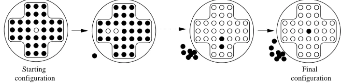
Peg solitaire is a peg game for one player which is played on a board containing a number of holes. The most common modern version uses a cross shaped board with 33 holes - see Fig. 1 - although a 37 hole board is common in France. Computer versions of the game now feature a wide variety of shapes, including rectangles and triangles. Initially the central hole is empty, the others contain pegs. If in some row (column respectively) two consecutive pegs are adjacent 1 _{Supported by NSERC Canada and FCAR Qu´ebec}

(2)

to an empty hole in the same row (column respectively), we may make amove

by removing the two pegs and placing one peg in the empty hole. The objective of the game is to make moves until only one peg remains in the central hole. Variations of the original game, in addition to being played on different boards, also consider various alternate starting and finishing configurations.

The game itself has uncertain origins, and different legends attest to its dis-covery by various cultures. An authoritative account with a long annotated

bibliography can be found in the comprehensive book of Beasley _{(4). The}

book mentions an engraving of Berey_{, dated 1697, of a lady with a}

Soli-taire board. The modern mathematical study of the game dates to the 1960s

at Cambridge University. The group was led by Conway _{who has written a}

chapter in (5) on various mathematical aspects of the subject. One of the

problems studied by the Cambridge group is the following basic feasibility

problem of peg solitaire:

For a given boardB, starting configuration cand finishing configuration c′

, determine if there is a legal sequence of moves fromc toc′

.

Final configuration

Starting

configuration

Fig. 1. A feasible English solitaire peg game with possible first and last moves

The complexity of the feasibility problem for the game played on a n by n

board was shown by Uehara and Iwata _{(11) to be NP-complete, so easily}

checked necessary and sufficient conditions for feasibility are unlikely to exist. One of the tools used to show the infeasibility of certain starting and finishing configurations is a polyhedral cone called thesolitaire cone SB, corresponding

to some given board B.

1.2 Basic properties

For ease of notation, we will mostly be concerned with rectangular boards which we represent by 0-1 matrices. A zero represents an empty hole and a one represents a peg. For example, let c =[ 1 0 1 1 ] and c′

=[ 0 0 1 0] be starting and finishing positions for the 1 by 4 board. This game is feasible, involving two moves and the intermediate position [ 1 1 0 0]. For any move

on an m by n board B we can define an m by n move matrix which has 3

(3)

and one entry of 1 for the hole receiving the new peg. The two moves involved in the previous example are represented by m1 =[ 0 1 -1 -1] and m2 =[ -1 -1 1 0]. Clearly c′

=c+m1+m2. By abuse of language, we use the term move for both the move itself and the move matrix. In general it is easily seen that if c, c′

define a feasible game ofk moves there exist move matricesm1, . . . , mk

such that c′ −c= k X i=1 mi. (1)

Clearly, Equation 1 is necessary but not sufficient for the feasibility of a peg game. For example, takec=[ 1 1 1 1 ] andc′

=[ 0 0 0 1]. We have c′

−c= [ -1 -1 1 0] + [ 0 1 -1 -1 ] + [ 0 -1 -1 1 ], butc, c′

do not define a feasible game; in fact there are no legal moves! Let us relax the conditions of the original peg game to allow a fractional (positive or negative) number of pegs to occupy any hole. We call this game the fractional game, and call the original game the 0-1 game (in a 0-1 game we require that in every position of the game a hole is either empty or contains a single peg). A fractional move matrix is obtained by multiplying a move matrix by any positive scalar and is defined to correspond to the process of adding a move matrix to a given position. For example, let c=[ 1 1 1], c′ =[ 1 0 1]. Then c′ −c=[ 0 -1 0 ] = 1 2 [ -1 -1 1] + 1 2 [ 1 -1 -1] is a feasible fractional game and can be expressed as the sum of two fractional moves, but is not feasible as a 0-1 game.

Let B be a board and nB the total number of possible moves on the board.

The solitaire cone SB is the set of all non-negative combinations of the nB

corresponding move matrices. Thus c′

−c∈SB if: c′ −c= nB X i=1 yimi, yi ≥0, i= 1, . . . , nB. (2)

In the above definition it is assumed that the hB holes in the board B are

ordered in some way and that c′

− c and mi are hB-vectors. When B is a

rectangular m by n board Bm,n it is convenient to display c′ −c and mi as

m by nmatrices, although of course all products should be interpreted as dot products of the corresponding mn-vectors. For n ≥4 or m ≥ 4, the solitaire cone Sm×n associated to the m by n board is a pointed full-dimensional cone

and the moves of the solitaire cone are extreme rays; see (3) for a detailed study of the solitaire cone. The following result obtained in 1961 is credited to Boardman _{(who apparently has not published anything on the subject)}

by Beasley _{(4), page 87. We identify} _c′

−cwith the fractional game defined by c and c′

.

Proposition 1 Equation 2 (c′

(4)

feasibility of the fractional game; that is, the solitaire cone SB is the cone of all feasible fractional games.

The condition c′

−c∈SB is therefore a necessary condition for the feasibility

of the original peg game and, more usefully, provides a certificate for the infeasibility of certain games. The certificate of infeasibility is any inequality valid for SB which is violated by c

′

−c. According to (4), page 71, these

inequalities “were developed by J.H. Conway and J.M. Boardman in 1961, and

were called pagoda functions by Conway...”. They are also known as resource

counts, and are discussed in some detail in Conway _{(5). The strongest such}

inequalities are induced by the facets of SB.

Other tools to show the infeasibility of various peg games include the so-called

rule-of-threewhich simply amounts to color the board by diagonals ofα,βand γ (in either direction). Then, with #α (#β,#γ resp.) denoting the number of pegs in an α-colored (β, γ resp.) holes, one can check that the parity of #α−#β, #β −#γ and #γ −#α is an invariant for the moves. The

rule-of-three was apparently first exposed in 1841 bySuremain de Missery_{; see}

Beasley_{’s book (4) for a detailed historical background. Another necessary}

condition generalizing the rule-of-three - the solitaire lattice criterion - is to check if c′

−c belong to the solitaire lattice generated by all integer linear combinations of moves, that is:

c′ −c= nB X i=1 yimi, yi ∈Z, i= 1, . . . , nB

While the lattice criterion is shown to be equivalent to the rule-of-three for the classical English 33-board and French 37-board as well as for anym×nboard, the lattice criterion is stronger than the rule-of-three for games played on more complex boards. In fact, for a wide family of boards the lattice criterion

exponentially outperforms the rule-of-three, seeDeza and Onn _(7).

The solitaire cone is generated by a set of extreme rays, each of which is all zero

except for three nonzero components which are 1,-1,-1. In Avis and Deza

(3), the solitaire cone is related to another cone with the same property, the

flow cone which is dual to the much studied metric cone which arises in the study of multicommodity flows; see, for example, (1; 6; 8; 10).

2 Facets of the Solitaire Cone

For simplicity we consider rectangular boards and, to avoid the special effects created by the boundary, we study their toric closures which are simply called

(5)

toric boards. In other words, the toric m by n board is an m by n rectangu-lar board with additional jumps which traverse the boundary. Note that the associated toric solitaire cone Sm×_n is pointed and full-dimensional for m≥3

orn ≥3. Let B be a rectangular m by n board, withm ≥3 or n≥ 3. Using

the notation described following equation 2, we will represent the coefficients of the facet inducing inequality

az ≤0 (3)

by the m by n array a = [ai,j]. Inequality 3 holds for every z ∈ Sm×n. It is a

convenient abuse of terminology to refer to a as a facet of Sm×n. Three

con-secutive row or column elements of an m by n array are denoted by (t1, t2, t3)

and called a consecutive triple of row or column indices. For example both

t1 = i, j, t2 = i, j + 1, t3 = i, j + 2 and t1 = i+ 2, j, t2 = i+ 1, j, t3 = i, j are consecutive triples. Using this notation we see that a move matrix for B is an m by n matrix that is all zero except for elements of some consecutive triple which take the values 1,-1,-1. Each consecutive triple defines a triangle inequality

at1 ≤at2 +at3 (4)

The definition of consecutive triple is extended by allowing row indices to

be taken modulo m and column indices to be taken modulo n. For example,

for a 4 by 4 toric board both t1 = 2,3, t2 = 2,4, t3 = 2,1 and t1 = 1,3, t2 = 4,3, t3 = 3,3 are consecutive triples. Similarly we extend the definition of a consecutive string of entries to include strings that traverse the boundary.

Fig. 2. Moves on the 4 by 4 toric board

The{0,1}-valued facets the solitaire cone are considerably more complex than the {0,1}-valued facets of the dual metric cone, which are generated by cuts

in the complete graph. For a toric board B, a complete characterization of

{0,1}-valued facets of Sm×n was given in (3). Let abe an m by n 0-1 matrix.

We define the 1-graph Ga on a as follows: vertices of Ga correspond to the

ones, and two ones are adjacent if the corresponding coefficients are in some consecutive triple where the remaining coefficient is zero. Note that in fact there must be at least two such triples since if (t1, t2, t3) is such a triple then so is (t3, t2, t1).

Theorem 2 LetB be them byn toric board. Ambyn 0-1 matrixa is a facet of Sm×n if and only if(i) no nonzero row or column contains two consecutive zeroes, and (ii) the 1-graph Ga is connected.

(6)

0 0 0 0 0 0 0 0 1 0 1 1 1 0 1 1 1 0 1 0 0 1 0 1 0 0 1 1 1 1 0 0

Fig. 3. Two pagoda functions ofS4×4, only the first one being a facet

Theorem 2 is useful for proving large classes of 0-1 matrices are facets. Let x = (x1, . . . , xm) and y = (y1, . . . , yn) be two vectors. We say the m by n

matrix a is the product of x and y if for all 1 ≤ i ≤ m and 1 ≤ j ≤ n

ai,j =xiyj. A simple application of Theorem 2 gives: Corollary 3

(1) Let B1,n be the 1 by n toric board. A {0,1}-valued n-vector is a facet of

S1×n if and only if it has no pair of consecutive zeroes, no string of five or more ones, and at most one string of four ones.

(2) LetBm,n be thembyn toric board. The product of two{0,1}-valued facets of S1×m and S1×n gives a {0,1}-valued facet of Sm×n.

Proposition 4 Let h(n) be the number of{0,1}-valued facets of S1×n.

For n≥7, (n+ 18)1.46n−8

≤h(n)≤(n+ 19)1.47n−6

.

PROOF. _{The formula can be verified directly for} _n _≤ ₁₁ _{by referring to}

the 5th _{column of Table 1. We define an} _f_{-vector to be a} _{₀_,₁_}_{-valued vector} of length n with no 2 consecutive zeroes, no string of 4 or more ones and starting and ending with a one. We first count f(n), the number of f-vectors. Direct calculation shows that: f(2) = 1, f(3) = 2, f(4) = 2, f(5) = 4. For

n ≥ 6, a f-vector has the form [1 0 1 ... 1], [ 1 1 0 1 ... 1 ] or [ 1 1 1 0 1 ... 1], where the string 1 ... 1 is an f-vector. In other words, we have

f(n) = f(n−2) +f(n−3) +f(n−4). It is easy to show by induction that for n≥6,

1.46n−₂

≤f(n)≤1.47n. (5)

Now, forn ≥12, by Item (1) of Corollary 3, the number h(n) of {0,1}-valued facets of S1×n is the number of toric {0,1}-valued vectors of length n with no 2 consecutive zeroes, no string of 5 or more ones, and at most one string of 4 ones. Call such vectors h-vectors. If an h-vector has no string of 4 ones, then it either starts with [ 0 1 ... 1], [ 1 0 1 ... ], [ 1 1 0 1 ... 1 0 ], [ 1 1 0 1 ... 1 0 1 ] or [ 1 1 1 0 1 ... 1 0 ] where the string 1 ... 1 is an f-vector. In other words, we have2f(n−1) +f(n−4) + 2f(n−5) = 2f(n−3) + 3f(n−4) + 4f(n−5) h-vectors without a string of 4 ones. We have nf(n−6) h-vectors with one string of 4 ones as each is of the form [ ... 1 0 1 1 1 1 0 1 ...]. Therefore, the

(7)

total number of h-vectors for n≥8 is given by

h(n) = 2f(n−3) + 3f(n−4) + 4f(n−5) +nf(n−6). (6)

The proposition follows by substituting the asymptotic bounds for f obtained above in this equation.

3 The Binary Solitaire Cone and Other relatives

The link with the dual metric cone and the similarities between their combina-torial structures - see (3) - leads to the study of a dual cut cone analogue; that is, the binary solitaire cone BSB generated by the {0,1}-valued facets of the

solitaire cone. We give some results and conjectures on the combinatorial and geometric properties of the binary solitaire cone. In particular we prove that

the extreme rays of SB are extreme rays of BSB strengthening the analogy

with the dual metric cone, for which the extreme rays are also extreme rays of the dual cut cone. Other related cones are also considered.

3.1 The binary solitaire cone

The dual cut cone is generated by the {0,1}-valued facets of the dual metric cone. Similarly, we consider the cone generated by the{0,1}-valued facets of the solitaire cone. This cone is calledbinary solitaire cone and denotedBSB.

We present in details some small dimensional cases and give some results and conjectures on the combinatorial and geometric properties of the binary soli-taire cone. In particular, we investigate the diameter, adjacency and incidence relationships of the binary solitaire cone BSm×_n and its dual BS

∗

m×n. Two

extreme rays (resp. facets) of a polyhedral cone are adjacent if they belong to a face of dimension (resp. codimension) two. The number of rays (resp. facets) adjacent to the ray r (resp. facet F) is denoted Ar (resp. AF). A ray and a

facet are incident if the ray belongs to the facet. We denote by Ir (resp. IF)

the number of facets (resp. rays) incident to the ray r (resp. facet F). The

diameter of BSB (its dual BS

∗

B resp.), that is, the smallest number δ such

that any two vertices can be connected by a path with at most δ edges, is

δ(BSB) (δ(BSB∗) resp.); see Table 1.

Finding all extreme rays of the cone BSB (such as the 930 048 rays ofBS4×4)

is an example of a convex hull or vertex enumeration problem, for which

various computer programs are available. The computational results in this

(8)

Table 1

Small binary toric boards

Board #rays Ir Ar #f acets IF AF δ(BSB) δ(BS_B∗)

1×3 3 2 2 3 2 2 1 1 1×4 8 3 3 6 4 4 3 2 1×5 15 4∼5 4∼5 10 6∼8 5∼7 3 2 1×₆ ₃₀ ₅∼₆ ₅∼₆ ₁₁ ₁₂∼₁₆ ₈∼₉ ₄ ₂ 1×₇ ₄₂ ₈∼₁₁ ₇∼₁₀ ₂₁ ₁₈∼₂₀ ₁₁∼₁₃ ₃ ₂ 1×₈ ₇₂ ₁₀∼₁₆ ₉∼₁₄ ₃₀ ₂₄∼₃₆ ₁₄∼₁₈ ₃ ₂ 1×₉ ₁₂₆ ₉∼₂₅ ₉∼₁₉ ₄₈ ₃₂∼₅₄ ₁₈∼₂₆ ₃ ₂ 1×₁₀ ₂₀₀ ₁₄∼₃₆ ₁₂∼₂₄ ₆₇ ₄₀∼₈₀ ₁₆∼₃₃ ₄ ₂ 1×₁₁ ₂₃₁ ₁₁∼₅₈ ₁₁∼₂₆ ₁₁₀ ₅₀∼₈₆ ₂₄∼₄₅ ₄ ₃ 1×12 516 12∼85 12∼51 159 60∼172 21∼62 4 3 3×3 18 11 15 15 12∼14 12∼14 2 2 4×₄ _{930 048} ₁₅∼₁₆₈ ₁₅∼_? ₃₄₀ _? _? _? _? 3×₄ _{1 284} ₁₁∼_{(30 34)} ₁₁∼₃₆₉ ₅₄ ₁₉₄∼₅₀₆ ₃₅∼₅₂ ₃ ₂ 3×₅ _{101 444} ₁₄∼_{(118 129)} ₁₄∼_{14 607} ₂₄₀ _? _? _? _?

Fukuda_{(9), and the reverse search method}_lrs_{implemented by}Avis_{(2). The}

diameters of cones were computed usinggraphyimplemented byFukuda_(9).

Theorem 5 The extreme rays of the solitaire cone, that is, the moves, are extreme rays of the binary solitaire cone.

PROOF. _{Given any extreme ray (move)} _c_of _S_m×n, let Φbe the intersection

of all the facets of BSm×n containing c. We want to prove that any vector

r∈Φ is a scalar multiple of c.

Case m ≤ 2. First, take m = 1. For n = 3, . . .12 Theorem5 was checked by computer so we can assume that n ≥ 13. All extreme rays of S1×n being equivalent up to scrolling and reversing, we can assume that c = [ -1 -1 1 0

. . . 0 ]. For j = 4, . . . , n, consider the two inequalities defined by f1

1jr≤0 and

f₁0_jr ≤0 as given bellow where the boxed value is the jth _coordinate

f₁1_j = 1,0,1,0,1,0. . . ,0,1,0,1, 1 ,1,0,1,0. . . f₁0_j = 1,0,1,0,1,0. . . ,0,1,0,1, 0 ,1,0,1,0. . .

Since the associated 1-graphs Gf1

1j and Gf

0

1j are connected, Theorem 2 gives

that those inequalities induce 2 facets F₁1j andF10j of BS1×n. As clearly f₁1_jc= f0

1jc= 0, we have F11j∩F10j ⊂Φ. Therefore, any vector r ∈Φ satisfies f11jr=

(9)

inequalities defined by f1,1r≤0 and f1,2r ≤0 as given bellow f1,1 = 0,1,1,0,1,0,1, . . . f1,2 = 1,0,1,0,1,0,1. . .

clearly induce 2 facets also belonging to Φ. It implies f1,1r = f1,2r = 0, that

is, r2+r3 =r1+r3 = 0. In other wordsr =r3×c; which completes the proof.

Since the case m= 2 is almost equivalent to the case m= 1, we next consider case m = 3.

Case m = 3. For n = 3,4,5 Theorem5 was checked by computer so we can assume that n ≥ 6. The two cases c′

1,1 = c

′

1,2 = −c

′

1,3 = −1 and c”1,1 = c”2,1 = −c”3,1 = −1 being essentially the same, we can assume that c = c′.

For i = 1,2,3 and j = 4, . . . , n, consider the inequalities defined by f_ij1r ≤ 0

(fij0r ≤ 0 resp.) as given bellow where the boxed value is the ijth coordinate. The coordinates of f_ij0 differ from f_ij1 only for the ijth _{coordinate which is set} to 0. fij1 =       1 0 1 1 . . . 1 0 1 1 0 1 1 1 0 1 1 0 . . . 0 1 1 0 . . . 0 1 1 0 1 1 1 0 1 1 0 1 . . . 1 1 0 1 . . . 1 1 0 1 1 1 0 1 1 0 1 1 . . .      

Similarly to the case m ≤ 2, the associated 1-graphs Gf1

ij and Gf

0

ij are

con-nected and, up to a rotation along the axis i = 2, we have f_ij1c′

= f_ij0c′

= 0; that is, the induced facets satisfy Fij1 ∩Fij0 ⊂ Φ. Therefore, any vector r ∈ Φ satisfies f1

ijr = fij0r = 0 for i= 1,2,3 and j = 4, . . . , n. This implies rij = 0 for i = 1,2,3 and j = 4, . . . , n. Slightly modified f_ij1 and f_ij0 for i = 2,3

and j = 1,2,3 give rij = 0 for i = 2,3 and j = 1,2,3. Moreover, the two inequalities defined by f1,1r≤0 and f1,2r ≤0 as given bellow

f1,1 =       1 0 1 0 1 . . . 0 1 0. . . 0 0 0 0 0 . . . 0 0 0. . . 1 0 1 0 1 . . . 0 1 0. . .       f1,2 =       0 1 1 0 1 . . . 1 0 1 . . . 0 0 0 0 0 . . . 0 0 0 . . . 0 1 1 0 1 . . . 1 0 1 . . .      

implies r1,1 =r1,2 =−r1,3, that is, r=r3×c′; which completes the proof.

Case m ≥ 4. Theorem5 was checked by computer for n = 4 so we can as-sume that n ≥ 5. We can take cij = 0 except c1,1 = c1,2 = −c1,3 = −1. For i= 3, . . . , m−1 or j = 4, . . . , n, consider the inequalities defined by fij1r ≤0 (f0

ijr ≤ 0 resp.) as given bellow where the boxed value is the ijth coordinate. The coordinates of f_ij0 differ from f_ij1 only for the ijth _{coordinate which is set}

(10)

to 0. f_ij1 =                                   1 0 1 0 . . . 0 1 0 1 0 1 1 1 0 1 0 0 . . . 0 0 0 0 . . . 0 0 0 0 0 0 0 0 0 0 0 0 . . . .. . ... ... ... · · · ... ... ... ... ... ... ... ... ... ... ... ... · · · 1 0 1 0 . . . 0 1 0 1 0 1 1 1 0 1 0 0 . . . 0 0 0 0 . . . 0 0 0 0 0 0 0 0 0 0 0 0 . . . 1 0 1 0 . . . 0 1 0 1 0 1 1 1 0 1 0 0 . . . 1 0 1 0 . . . 0 1 0 1 0 1 1 1 0 1 0 0 . . . 1 0 1 0 . . . 0 1 0 1 0 1 1 1 0 1 0 0 . . . 0 0 0 0 . . . 0 0 0 0 0 0 0 0 0 0 0 0 . . . 1 0 1 0 . . . 0 1 0 1 0 1 1 1 0 1 0 0 . . . .. . ... ... ... · · · ... ... ... ... ... ... ... ... ... ... ... ... · · ·                                   Clearly, we have f1

ijc=fij0c= 0. By filling the gaps with the following {0,1} -valued matrices (or their transposes), the associated 1-graphs Gf1

ij and Gf

0

ij

are both connected. Therefore, any vector r ∈ Φ satisfies rij = 0 for i =

3, . . . , m−1 or j = 4, . . . , n.              1 0 1 0 . . . 1 0 1 1 1 0 1 0 . . . 0 0 0 0 . . . 0 0 0 0 0 0 0 0 . . . 1 0 1 0 . . . 1 0 1 1 1 0 1 0 . . . 0 0 0 0 . . . 0 0 0 0 0 0 0 0 . . . .. . ... ... ... · · · ... ... ... ... ... ... ... ... · · ·                           1 0 1 0 . . . 1 0 1 1 1 0 1 0 . . . 1 0 1 0 . . . 1 0 1 1 1 0 1 0 . . . 0 0 0 0 . . . 0 0 0 0 0 0 0 0 . . . 1 0 1 0 . . . 1 0 1 1 1 0 1 0 . . . .. . ... ... ... · · · ... ... ... ... ... ... ... ... · · ·             

Slightly modified fij1 and fij0 for i = 2, m and j = 1,2,3 give rij = 0 for

i= 2, m and j = 1,2,3. For example, the following inequalities set r2,2 to 0

f₂1_,₂ =                 0 1 1 1 0 1 0 1 . . . 1 1 1 0 1 0 1 0 . . . 0 1 0 1 0 1 0 1 . . . 1 0 1 0 1 0 1 0 . . . 0 1 0 1 0 1 0 1 . . . .. . ... ... ... ... ... ... ... · · ·                 f₂0_,₂ =                 0 1 1 1 0 1 0 1 . . . 1 0 1 0 1 0 1 0 . . . 0 1 0 1 0 1 0 1 . . . 1 0 1 0 1 0 1 0 . . . 0 1 0 1 0 1 0 1 . . . .. . ... ... ... ... ... ... ... · · ·                

(11)

Finally, the following two inequalities set r1,1 =r1,2 =−r1,3, f1,1 =              1 0 1 0 1 . . . 0 0 0 0 0 . . . 1 0 1 0 1 . . . .. . ... ... ... ... · · · 0 0 0 0 0 . . .              f1,2 =              0 1 1 0 1 . . . 0 0 0 0 0 . . . 0 1 1 0 1 . . . .. . ... ... ... ... · · · 0 0 0 0 0 . . .             

that is, r=r3×c; which completes the proof.

Corollary 6 The binary solitaire cone is full-dimensional.

Out of the 930 048 extreme rays ofBS4×4, the 64 extreme rays ofS4×4, that

is, the moves, reached the highest incidenceImax

r = 168 which is almost three

times larger than the second highest incidence Isubmax

r = 57. Similarly, out

of the 101 444 extreme rays of BS3×5, the 15 vertical moves of S3×5, reached

the highest adjacency Amax

r = 14 607 while the average adjacency is Aaver ≃

33.16. These computational results and other similarities with the metric cone - see (3) - lead us to the following conjectures:

Conjecture 7

(1) For n ≥ 3 and m ≥ 3, the moves form a dominating set in the skeleton of BSm×n.

(2) The incidence of the moves is maximal in the skeleton of BSm×n.

(3) For m, n large enough, at least one ray r of BSm×n is simple, (that is,

Ir =mn−1).

Item (1) of Conjecture 7 holds forBS3×4 and is false for m≤2. The smallest

1 bynboard for which the conjecture fails is the 1 by 10 board. Item (2) holds for all cones presented in Table 1 and is false if we replace the incidence by the adjacency as, for example, for BS3×5. If true, Item (3) would imply that

the edge connectivity, the minimal incidence and the minimal adjacency of the skeleton ofBSm×n are equal to nm−1. This holds for BS3×₄, BS₃×₅ and BS4×4.

3.2 The trellis solitaire cone

The{0,1}-valued facets of the solitaire cone have much less structure than the set of cut metrics. In fact, the cut metrics are related to products of vectors of length n. This motivates the next definition. Let f and g be {0,1}-valued

(12)

vectors of length m and n respectively, and let cij = fi ·gj for i = 1, . . . m,

j = 1, . . . n. Ifc·x≤0 defines a facet of BSm×n, we call it atrellis facet. The trellis solitaire cone TSB is generated by all of thetrellis facets of the binary

solitaire cone BSB. See Item (2) of Corollary 3 for an easy construction of

trellis facets. For example, among the two following facets of BS3×₅, only the

right one is a trellis facet.

1 0 0 1 0 0 1 0 0 0 1 0 0 1 1 1 1 1 0 0 0 0 1 1 0 1 1 1 1 1

Fig. 4. A facet and a trellis facet ofBS3×₅

Conjecture 8 The binary trellis solitaire cone is full-dimensional.

3.3 The complete solitaire cone

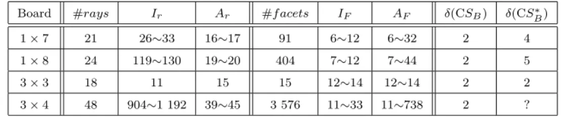
The complete solitaire cone CSB is induced by a variation of the Solitaire

game. To the classical moves we add the moves which consist of removing two pegs surrounding an empty hole and placing one peg in this empty hole as shown in Fig. 5. The incidence and adjacency relationships and diameters of small dimensional complete solitaire cones are presented in Table 2. Two rays

r

0 -1 1 -1 0

C C’

Fig. 5. The extreme rayr of CS1×₅ corresponding to the move fromc toc ′

Table 2

Small complete toric boards

Board #rays Ir Ar #f acets IF AF δ(CSB) δ(CSB∗)

1×₇ ₂₁ ₂₆∼₃₃ ₁₆∼₁₇ ₉₁ ₆∼₁₂ ₆∼₃₂ ₂ ₄

1×₈ ₂₄ ₁₁₉∼₁₃₀ ₁₉∼₂₀ ₄₀₄ ₇∼₁₂ ₇∼₄₄ ₂ ₅

3×₃ ₁₈ ₁₁ ₁₅ ₁₅ ₁₂∼₁₄ ₁₂∼₁₄ ₂ ₂

3×₄ ₄₈ ₉₀₄∼_{1 192} ₃₉∼₄₅ _{3 576} ₁₁∼₃₃ ₁₁∼₇₃₈ ₂ _?

are calledstrongly conflictingin there exist two pairsi, j andk, lsuch that the two rays have nonzero coordinates of distinct signs at positions i, j and k, l (respectively i, j). We have CS3×3 = S3×3 and, by analogy with the classical

solitaire cone case, we conjecture:

Conjecture 9 For n ≥ 7 and m ≥ 7 a pair of extreme rays of CSm×n are adjacent if and only if they are not strongly conflicting.

(13)

3.4 The binary complete solitaire cone

In the same way as we did for the solitaire cone, we consider the cone generated by the facets of the complete solitaire cone CSBwhose coordinates are, up to a

constant multiplier,{0,1}-valued. This cone is calledcomplete binary solitaire cone and denoted BCSB. The incidence and adjacency relationships of small

dimensional complete binary solitaire cones BCSB are presented in Table 3.

Table 3

Small binary complete toric boards

Board #rays Ir Ar #f acets IF AF δ(BCSB) δ(BCS∗_B)

1×₇ ₇ ₆ ₆ ₇ ₆ ₆ ₁ ₁

1×8 16 9 10 12 12 9∼10 2 2

3×3 18 11 15 15 12∼14 12∼14 2 2

3×₄ ₇₂ ₁₄∼₂₈ ₁₅∼₅₈ ₃₆ ₃₀∼₄₅ ₃₀∼₃₅ ₂ ₂

4 Conclusion

Theorem 5 strengthens the analogy of the solitaire cone with the dual metric cone, for which the extreme rays are also extreme rays of the dual cut cone. On

the other hand, so far we have not yet found an analogue of the hypermetric

facets of the metric cone Mn, that is, a “nice” family of {0,−1,1}-valued

extreme rays of the binary solitaire cone BSB. Another open question is the

determination of a tighter relaxation of the solitaire cone SB by some cuts analogue. The trellis solitaire cone TSB is a candidate as well as the cone

generated by the {0,1}-valued facets with the minimal number of ones. For S4×₄ and S₃×i :i= 3,4,5, these facets have maximal incidence and adjacency

in the skeleton of S∗

m×n.

References

[1] Avis D.: On the extreme rays of the metric cone. Canadian Journal of

Mathematics XXXII1 (1980) 126–144

[2] D. Avis,lrs, A revised implementation of the reverse search vertex enu-meration algorithm, (1998) ftp://mutt.cs.mcgill.ca/pub/doc/avis/ [3] D. Avis and A. Deza, On the solitaire cone and its relationship to

multi-commodity flows,Mathematical Programming 90-1 (2001) 27–57.

[4] J. D. Beasley, The Ins and Outs of Peg Solitaire (Oxford University

Press 1992).

(14)

Prop-erly, Winning Ways for your mathematical plays, 2 Academic Press (1982) 697–734.

[6] A. Deza, M. Deza and K. Fukuda, On skeletons, diameters and

vol-umes of metric polyhedra, Combinatorics and Computer Science,

Lec-ture Notes in Computer Science 1120 Springer-Verlag, Berlin (1996) 112–128.

[7] A. Deza and S. Onn, Solitaire lattices, Graphs and Combinatorics (to

appear).

[8] M. Deza and M. Laurent, Geometry of cuts and metrics,Algorithms and

Combinatorics 15 Springer-Verlag, Berlin (1997).

[9] K. Fukuda, cdd/cdd+ reference manual 0.75, ETHZ, Z¨urich, Switzerland

(1997).

[10] M. Lomonosov, Combinatorial Approaches to Multiflow Problems,

Dis-crete Applied Mathematics11 (1985) 1–93.

[11] R. Uehara and S. Iwata, Generalized Hi-Q is NP-complete,Trans. IEICE