A general formula for the method of steepest descent using
Perron’s formula
James Mathews
December 16, 2013
1
Introduction
The method of steepest descent is one of the most used techniques in applied mathematics and asymptotics, but is often one of the hardest to apply. We want to find an approximation for the integral
I(k) =
Z
C
g(z)ekf(z)dz ask → ∞
where f and g are (usually) analytic functions, k is (usually) a real parameter. The general idea is to use Cauchy’s theorem which allows deformation of contours in the complex plane to simplify the problem. The idea was proposed by Debye, and the basic idea is to choose a new contour D
such that
• D passes through one of more zeros off0(z)
• The imaginary part off(z) is constant onD
Since the imaginary part of the integral is constant, then iff(z) =g(z) +ihthen we instead need to evaluate.
I(k)eikh
Z
C
g(z)ekg(z)dz as k → ∞, which can then be treated by Laplace’s method.
1.1
Laplace’s method
Laplace’s method says that to evaluate J(k) =
Z b
a
f(t)ekφ(t)dt ask → ∞,
where φ(t) has a stationary point at an interior point c with non-zero second derivative (so f0(t) = 0 and f00(t)6= 0), then J(k)∼ √ 2πf(c)exφ(c) p −kφ00(c) . 1
Ifc is in fact an end point then we need to multiply this expression by a factor of 1/2. If in fact we have no stationary point then we have
J(k)∼ −f(a)e kφ(a) kφ0(a) , or J(k)∼ f(b)e kφ(b) kφ0(b) ,
with the first case corresponding to the maximum of φ being at a, so φ0(a)< 0, and the second corresponding to the maximum being at b, so φ0(b)>0.
Finally, if cis a maximum with φ0(c) =φ00(c) =. . . φp−1(c) = 0 and φp(c)<0 then we get
J(k)∼ 2Γ(1/p)(p!)
1/p
p[−kφp(c)]1/p f(c)e xφ(c)
.
See [Bender and Orszag, 1978] for the proofs and examples of this method.
1.2
Difficulties with the method
The main difficulty of the method, is of course, finding the new contour. We suppose the contour is not closed, and has end points a and b. Often, this contour consists of three parts;
• D1 which goes through a and has imaginary part =[f(a)]
• D2 which goes through b and has imaginary part =[f(b)]
• D3 which joins the two contours at ‘infinity’
It is hoped that the contribution of the integral from D3 will become zero as D3 becomes more ‘infinite’, whilst the other two contours are evaluated using Laplace’s method. The examples in [Bender and Orszag, 1978] show how to apply the procedure, with the latter examples showing just how complicated the contours become. Whilst we can always apply this method, it can be time consuming, intricate and often we would just like a general formula to be able to estimate, say the leading behaviour.
Also, sometimes our function f will depend on another parameter, say λand we want to know what the asymptotic approximation is as we vary over λ. Rather than having to find various curves of steepest descent, which will depend on λ and properties might change dramatically, if we have a general formula then it will be easier.
Essentially, we want to use reasoning somewhat similar to Laplace’s method; we find where the function<[f(z)] has a maximum (or maximum’s) along a chosen contour, then sincekis large the only contributions to the integral will come from these points.
1.3
First (wrong) attempt at a general formula
A naive way to estimate the leading order behaviour is given below. It is based upon the notes sad, which is one of the first results you come across on google for saddle point methods. The method suggests that ifz0 is a (non-degenerate) saddle point, then
I(k) = Z C g(z)ekf(z)dz ∼ 2π k|f00(z 0)| 1/2 g(z0)ekf(z0)exp i π 2 − arg(f00(z0)) 2 . The reasoning given seems clear; you approximatef(z) by its Taylor expansion atz0 so
f(z)≈f(z0) + 1 2f
00
(z0)(z−z0)2 and g(z) by g(z0), then we just need to evaluate
I(k)≈g(z0)ekf(z0) Z expk 2f 00 (z0)(z−z0)2dz. (1.1)
We then switch to polar coordinates, extend the limits and perform the Gaussian integral to get the result. All this reasoning looks clear, until we examine it further and note two glaring problems:
• At no point did we use the fact thatk is large, how can we construct an asymptotic approx-imation without using this property!?
• Just because f0(z0) = 0 does not mean that the real part of f(z) is maximised at z0. These are in fact linked as explained above, we find where the real part of f(z) is maximised and then use the fact that k is large to show the only contribution to the integral is at this part. The argument above fails when we try and evaluate the integral in (1.1).
1.4
Example 1
We end this section with a simple example showing why the general formula is useful, and why our first attempt is wrong. We consider the integral
Z 1
−1
ek(z2−2iz)dz.
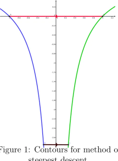
We can calculate thatf(z) =z2−2iz has a saddle point at z =i. The first attempt then suggest that the general behaviour can be calculated by only consideringf(z) near the saddle point. But we can see that
f(−1) = 1 + 2i, f(i) = 1, f(1) = 1−2i
and at both end points and the saddle point <[f(z)] = 1, so we must consider the contribution from all the points, even though the endpoints are not saddle points.
Figure 1: Contours for method of Using the formula we would say
Z 1 −1 ek(z2−2iz)dz ∼i r π ke k ,
which as we will see later, is plain wrong! If instead we try and solve the problem using the standard method of steepest descent, the contours we get are not so nice, but it will be possible to solve it. We can also see from Figure 1 that there is going to very hard to pass through the saddle point using only curves of constant phase. In the Figure the curves of constant phase going through the points−1 and 1 are drawn in blue and green respectively.
2
A general formula
As our example clearly showed, the most important issue is showing that any pointz0 we choose to approximate our integral at satisfies<[f(z)−f(z0)]<0 for allzon the contour we are integrating over, so we can in effect use Lapace’s method. This critical condition, so often overlooked is the main point of this notes. If in fact <[f(z)−f(z0)] = 0 for all z on the contour, then we can simply use the method of stationary phase, which is detailed in [Bender and Orszag, 1978]. Our basic idea will be
• If <[f(z)] is maximised at one of the end points (or even both) then we can simply use Perron’s Formula.
• If not, we find the saddle points of f, that is the points ci which satisfy f0(ci) = 0. We
then deform the contour C to a new contour D which goes through the saddle points in the direction of steepest descent.
• We find the asymptotic points, that is the solutions to <[f0(zi)] = 0, for zi which lie
on the contour D, which has end points a and b. We also include a and b as asymptotic points.
• We order the zi into increasing order along the deformed contour (so if we start at a then
as we go along the contour to b we will pass through the points in the order z1, z2, . . . zn).
• We then split the deformed contourD in contoursD[a,z1],D[z1,z2], . . .C[zn,b], and if there is no
zi then we simply take the deformed contour.
• Note that on each contour we have <[f(z)−f(w)] < 0 for all z on the contour D[zi,zi+1],
wherew is either zi and zi+1.
• We evaluate each of these integrals using Perron’s formula.
In the case where<[f(z)] is maximised at both end points a and b, we spilt the integral into two integrals by choosing an arbitary pointc∈(a, b) and then applying Perron’s formula to both. We assume that the<[f(z)] has only finitely many maxima and minima, and don’t consider the case where we have infinitely many. We do this because it is unlikely the standard method of steepest descent would cope with this method.
We also briefly recap how to find the direction of steepest descent at a saddle point c. If f is analytic at the critical point with f0(c) = f00(c) = . . . = f(N−1)(c) = 0 and f(N) = reiθ (with r >0) then the paths of steepest descent have direction
(2n+ 1)π−θ
N for n= 0,1, . . . N.
In the case N = 2 (so a non-degenerate saddle point) the paths of steepest descent have direction (π−θ)/2 and (3π−θ)/2.
2.1
Perron’s Formula
All that remains to be done is to evaluate integrals of the type I(k) =
Z
E
g(z)ekf(z)dz, (2.1)
whereE is a generic contour with end pointsaandb, and<[f(z)−f(w)]<0 wherewis eitheraor b. For simplicity we assume that it is at afor now. We now state Perron’s formula (first described by Oscar Perron in 1917) in the case that k is a real parameter, although with more assumptions we can state if for complex k. We also restrict to the case where f is analytic everywhere (or at least analytic at every zi), which again simplifies the assumptions for the Theorem. The full
theorem is stated in [Wong, 2001] and [Nemes, 2012], as well the proof, which we will not present here.
Theorem 2.1 (Perron’s Method) Assume that
1. D lies in the sector |arg(f(a)−f(z))| ≤π/2−δ for some fixed δ >0
2. For all c6=a onD, there exists fixedε(z)>0such that |f(z)−f(a)| ≥ε(z) for all z on the contour between z =c and z =b.
3. In a neighbourhood of a, f(a)−f(z) = ∞ X n=0 an(z−a)n+α,
where α∈N (since we have assumed f is analytic) and a0 6= 0.
4. In a neighbourhood of a, g(z) = ∞ X n=0 bn(z−a)n+β−1, where β >−1 and b0 6= 0.
5. The integral (2.1) exists absolutely for each fixed k
Let
w= lim
z∈D→aarg(z−a),
then we require that for some fixed l we have the following inequality holds (to ensure the first condition holds) 2l− 1 2 π+δ≤arga0+αw≤ 2l+ 1 2 π−δ. Then I(k)∼ekf(a) ∞ X s=0 ηs k(s+β)/αΓ s+β α e2πil(s+β)/α, (2.2) where ηs= 1 αa(0s+β)/αs! s X m=0 bs−m m! " d dzm ( a0(z−a)α f(a)−f(z) (s+β)/α)# z=a (2.3) The first two conditions are a slight strengthening of the condition<[f(z)−f(a)]<0, and can in most case be replaced by this condition. The third condition relates to the Taylor expansion of f at a, and we can see that if a is not a saddle point then α = 1, ifa is a non-degenerate saddle point (f0(a) = 0 and f00(a)6= 0) then α= 2, and otherwise if f0(a) = f00(a) = . . .=f(n−1)(a) = 0 and f(n)(a)6= 0 then α=n. Note also that
a0 =−f(α)(a)/α!, a1 =−f(α+1)(a)/(α+ 1)! and an=−f(α+n)(a)/(α+n)!,
with the minus sign just comes since the left hand side is f(a)−f(z) and not f(z)−f(a). If g is analytic at a and g(a) 6= 0, then β = 1 and b0 = g(a). Otherwise if g is analytic and g0(a) = g00(a) = . . .=g(m−1)(a) = 0 and g(m)(a)6= 0 then we have β =m, and then
b0 =g(β−1)(a)/(β−1)!, b1 =g(β)(a)/β! and bn=g(β+n−1)(a)/(β+n−1)!.
The fifth condition ensures that the asymptotic approximation will make any sense!
2.1.1 The first two coefficients
Assuming that g is analytic, then we can calculate that the coefficient of leading order, η0, will be given by η0 = b0 αaβ/α0 = g(β−1)(a)(α!)β/α α(β−1)![−f(α)(a)]β/α,
while the second coefficient is given by η1 = b1 αa(1+0 β)/α − (1 +β)b0a1 α2a(1+α+β)/α 0 = g (β)(a)(α!)(1+β)/α αβ/α + (1 +β)g(β−1)(a)f(α+1)(a)(α!)(1+β)/α (β−1)!α2(α+ 1)[−f(α)(a)](1+α+β)/α,
with subsequent coefficients becoming more and more complicated. I think the third coefficient is given by η2 = 1 αa(2+0 β)/α b2−b1(2 +β)a1 αa0 − b0 2 2 +β α 2a2 a0 − 2 +β α + 1 a1 a0 2.1.2 Maximum at b
If instead we have the maximum of the real part of f being at b rather than a, then the formula is modified slightly. We replace Conditions 3 and 4 in Theorem 2.1 by the conditions
3*. In a neighbourhood of b, f(b)−f(z) = ∞ X n=0 cn(b−z)n+α, whereα ∈Nand c0 6= 0. 4*. In a neighbourhood of b, g(z) = ∞ X n=0 dn(b−z)n+β−1, whereβ >0 and d0 6= 0. Then we have I(k)∼ekf(b) ∞ X s=0 ηs k(s+β)/αΓ s+β α e2πil(s+β)/α, (2.4) but we replace (2.3) by ηs = 1 αc(0s+β)/αs! s X m=0 ds−m(−1)m m! " d dzm ( c0(b−z)α f(b)−f(z) (s+β)/α)# z=b (2.5) 6
We can caclulate that if g is analytic then we have cn= (−1)α+n−1f(α+n)(b) (α+n)! and dn= (−1)β+n−1g(β+n−1)(b) (β+n−1)! .
In the case of the maximum being at the end point b, we can calculate that the coefficient of leading order, η0, will be given by
η0 = d0 αcβ/α0 =
(−1)(β−1)g(β−1)(a)(α!)β/α
α(β−1)![(−1)(α−1)f(α)(a)]β/α.
2.2
Special case: Contour is on the real line
In the case where the contour is on the real line, w = 0 thus we have l = 0. Furthermore, if we assume that g is analytic at a with g(a)6= 0 then β= 1 and to leading order we have
I(k)∼ekf(a)g(a)Γ(1/α)(α!) (1/α)
α[−f(α)(a)]1/αk1/α +e
kf(a)g(a)Γ(1/α)(α!)(1/α)
α[−f(α)(a)]1/αk1/α (2.6)
when the maximum is at the endpoint a. If instead g is analytic atb with g(b)6= 0 then we have
I(k)∼ekf(b) g(b)Γ(1/α)(α!) (1/α)
α[(−1)(α−1)f(α)(b)]1/αk1/α, (2.7)
when the maximum is at the endpointb.
2.3
Other attempts at a General Formula
The same result is proved in [Ferreira et al., 2007], under the same conditions, although they only calculate the order of the terms in the approximation, and not the constants (although the coefficients can be calculated using Laplace’s method). The paper would also seem to suggest that the method is uniform in the sense that if f depends on a parameter that changes, then the approximation is uniformly valid.
In Sections 3 and 4 of [Ferreira et al., 2007], the authors suggest a different way to deal with multiple asymptotic points, rather than splitting the contour up. However, both methods still rely on calculating the asymptotic points, and in my opinion the method we have presented here is easier.
2.4
Example 1 (revisited)
Returning to the example before, we can see that<[f(z)] = z2has a maximum at both end points. We choose to split the integral at the point 0, but this is arbitary, and so we have
I(k) = Z 1 −1 ek(z2−2iz)dz =I1(k) +I2(k), where I1(k) = Z 0 −1 ek(z2−2iz)dz and I2(k) = Z 1 0 ek(z2−2iz)dz. 7
Now I1 is of the form (2.6) since the maximum occurs at the lower of the limits, and since f(−1) = 1 + 2iand f0(−1) =−2−2i we have α= 1 and hence
I1(k)∼
ek(1+2i) (2 + 2i)k.
Similarly, I2 is of the form (2.7) since the maximum occurs at the upper of the limits, and since f(1) = 1−2i and f0(1) = 2−2i we have α = 1 and hence
I1(k)∼ e k(1−2i) (2−2i)k. Thus I(k)∼ e k(1+2i) (2 + 2i)k + ek(1−2i) (2−2i)k = ek 2k[sin(2k) + cos(2k)]. Below we plot I(k)/{ek
2k[sin(2k) + cos(2k)]}, and shows that the asymptotic approximation we
have chosen is indeed an asymptotic relation!
0 50 100 150 200 250 300 350 400 450 500 550 600 0.5 1 1.5 2 k
The spikes are caused by the fact that the zeros ofI(k) and e2kk[sin(2k) + cos(2k)] don’t quite line up until k gets large, but either way we have shown our method is easy to use for this example, and significantly easier than the standard method of steepest descent.
2.5
Example 2
We now take the example
I(k) = Z 2 −2 1 z−2ie k(2iz−z2) dz,
This has asymptotic points at−2, 0 and 2 sincef0(z) = 2i−2z. Suppose we just split the integral up up into two integrals, I1 between −2 and 0 and I2 between 0 and 2. This is not what out method says, but we try it anyway. Using Perron’s method we see that α = β = 1 at the end point 0, and furthermoref(0) = 0,f0(0) = 2i and g(0) =i/2. Hence we have
I1(k)∼ 1
4k and I2(k)∼ − 1 4k, 8
and hence when we sum the two asymptotic approximations they cancel! Furthermore, if we take the next term in Perron’s method (using f00(0) =−2 and g0(0) = 1/4 we have that
I1(k)∼ 1 4k + 3 16k2 and I2(k)∼ − 1 4k − 1 16k2,
and they still cancel! We can numerically calculate the integral whenk = 20 as I(k)≈7.97i×10−10,
which is what we don’t see at all from using Perron’s method. The trouble is that the imaginary behaviour of the integral is asymptotically small compared to the real part, so we don’t see it!
Thus, we should deform the contour to go through the critical point in the direction of steepest descent first before worrying about splitting the integrals up. The critical point lies at z =i, so we deform the contour to go throught this point. To keep things simple, we have the new contour going from−2 to−2 +i, from−2 +i to 2 +iand then from 2 +ito 2. We can check that indeed we have gone through the critical point in the direction of steepest descent. Thus, we need to evaluate the integrals
I1(k) = Z −2+i −2 1 z−2ie k(2iz−z2) dz, I2(k) = Z i −2+i 1 z−2ie k(2iz−z2) dz and I3(k) = Z 2+i i 1 z−2ie k(2iz−z2) dz, I4(k) = Z 2 2+i 1 z−2ie k(2iz−z2) dz. We can write the second and third integrals as
I2(k) = Z 0 −2 1 x−ie k(−x2−1) dx, and I3(k) = Z 2 0 1 x−ie k(−x2−1) dx, and then using Perron’s method (or even just Laplace’s method) we can calculate
I2(k)∼ i√π 2√ke −k and I 3(k)∼ i√π 2√ke −k.
We can write the first and fourth integrals as I1(k) =i Z 1 0 1 ix−2−2ie k[x2−2x−4+4i(x−1)] dx, and I4(k) = −i Z 1 0 1 ix+ 2−2ie k[x2−2x−4+4i(1−x)] dx, and then using Perron’s method with α = 1, β = 1 since they both have the real part of the exponentianted function having amaximum at the end pointx= 0 we have
I1(k)∼e−4k−4ik i 4(i−3)k and I4(k)∼ −e −4k+4ik i 4(3 +i)k and hence I1(k) +I4(k)∼ e−4ki 4k e−4ik i−3− e4ik i+ 3 =−e −4ki 20k (sin(4k) + 3 cos(3k)),
and hence is expoentially smaller than contributions from I2 and I3. Hence, we get the correct asympotic behavour of I(k)∼ i √ π √ k e −k. 9
References
Saddle point notes. http://www2.ph.ed.ac.uk/~dmarendu/MOMP/lecture05.pdf. Accessed: 21-10-2013.
Carl M Bender and Steven A Orszag. Advanced mathematical methods for scientists and engineers I: Asymptotic methods and perturbation theory, volume 1. Springer, 1978.
Chelo Ferreira, Jos´e L L´opez, Pedro Pagola, and E P´erez Sinus´ıa. The laplaces and steepest descents methods revisited. In Int. Math. Forum, volume 2, pages 297–314, 2007.
Gergo Nemes. Asymptotic expansions for integrals. 2012.
Roderick Wong. Asymptotic approximation of integrals, volume 34. SIAM, 2001.