Quantifying information transfer and mediation along causal pathways in complex systems
Jakob Runge*Potsdam Institute for Climate Impact Research, P. O. Box 60 12 03, 14412 Potsdam, Germany and Department of Physics, Humboldt University, Newtonstr. 15, 12489 Berlin, Germany
(Received 10 August 2015; revised manuscript received 23 October 2015; published 28 December 2015) Measures of information transfer have become a popular approach to analyze interactions in complex systems such as the Earth or the human brain from measured time series. Recent work has focused on causal definitions of information transfer aimed at decompositions of predictive information about a target variable, while excluding effects of common drivers and indirect influences. While common drivers clearly constitute a spurious causality, the aim of the present article is to develop measures quantifying different notions of the strength of information transfer along indirect causal paths, based on first reconstructing the multivariate causal network. Another class of novel measures quantifies to what extent different intermediate processes on causal paths contribute to an interaction mechanism to determine pathways of causal information transfer. The proposed framework complements predictive decomposition schemes by focusing more on the interaction mechanism between multiple processes. A rigorous mathematical framework allows for a clear information-theoretic interpretation that can also be related to the underlying dynamics as proven for certain classes of processes. Generally, however, estimates of information transfer remain hard to interpret for nonlinearly intertwined complex systems. But if experiments or mathematical models are not available, then measuring pathways of information transfer within the causal dependency structure allows at least for an abstraction of the dynamics. The measures are illustrated on a climatological example to disentangle pathways of atmospheric flow over Europe.
DOI:10.1103/PhysRevE.92.062829 PACS number(s): 89.75.Fb,89.70.Cf,02.50.−r,05.45.Tp I. INTRODUCTION
The availability of vast amounts of time-series data from such complex systems as the Earth or the human brain and body has given rise to a plethora of time-series analysis meth-ods aimed at understanding interactions between regions or subprocesses in these complex systems. Of particular interest are methods to quantify some notion ofinformation flowor in-formation transferwithin the complex system. In neuroscience [1] and climate research [2,3], such interpretations have often been based on pure pairwise correlation analyses. But towards measuring information transfer, the method should, first, be general enough to include also nonlinear associations. This can be achieved in an information-theoretic framework with mea-sures such as mutual information (MI) [4]. Second, networks reconstructed from pairwise measures of association (be it cross-correlation or MI) do not allow to assess the propagation of information or hypothetical perturbations in a causal sense: For example, an interaction likeX←Z→Y would imply that X and Y are correlated even though no perturbations originating inXcan actually reachY or vice versa.
An important step towards deeper insights has, therefore, been achieved by methods that are capable of inferring a statistical notion of directionality or even causal interactions which have been applied to the climate system [5–10] and the human brain [11–13] and to disentangle cardiovascular processes [14–16], among others. Causal associations between subprocesses can be visualized as links in a complex interac-tion network. A full causal reconstrucinterac-tion of a linkX→Y
can only be achieved under the, in most cases, unrealistic assumption that all possible other influences on X and Y
can be included in the analysis [17,18] or if the system can
*Corresponding author: [email protected]
be experimentally manipulated within Pearl’s causal effect framework [19]. Usually, it is impossible to exclude all other influences and large complex systems can typically not be easily experimentally manipulated. Causal inference based on data-analysis methods, therefore, provides only a first step and the term “causal” can then only be understood to be meant relative to the system under study, i.e., the processes that comprise the nodes of the network.
Two tasks need to be addressed to measure a causal notion of information transfer from time series of complex systems: (i) reconstructing the causal network and (ii) quantifying causal information transfer.
In this article we will focus on the quantification part, as the reconstruction problem has been addressed by the author in Ref. [20]. As further reviewed below, previous works have mainly considered a decomposition of the predictive information in direct drivers of a process Y. In the present article, we ask a different question: How does information originating in a process X propagate also on indirectpaths through the causal interaction network? How strong is it and which intermediate processes on causal pathways are contributing to such a mechanism?
The paper is organized as follows: In the remainder of this introductory section, we review recent approaches to measuring information transfer in complex systems and sketch the basic idea underlying the present approach. In Sec.IIwe recall basic concepts of information theory and in Sec. III
introduce the concept oftime-series graphsas the causal basis of the present approach. In Sec.IV we introduce the novel measures based on time-series graphs to quantify interactions along paths and mediation and distinguish them from transfer entropy-related approaches. In Sec.Vwe extensively analyze the measures with analytical and numerical examples and provide theorems that foster a more rigorous mathematical and dynamical understanding to facilitate the interpretability
of the proposed measures. SectionVIdiscusses the theoretical results and relation to linear measures of causal effect in Pearl’s framework [21] and gives an outlook to applications of the novel measures in complex network theory. Finally, Sec.VII
gives an illustrative application to climatological time series and Sec. VIII concludes the paper. The Appendix contains proofs of the theorems.
A. Quantifying causal information transfer
Compared to the first task of detecting causal interactions, more or less a binary question, the second task of quantifying causal information transfer is much more ambiguous to define in a universal way which has led Smirnov [22,23] to question the goal of assessing a “causal coupling strength” and instead measure “how the coupling manifests itself in the dynamics” in aninterventional-effectcausal framework as proposed by Pearl [19]. In Ref. [24] the term “information transfer” is even distinguished from “information flow” where the latter is meant in a causal sense based on interventions. This framework, however, necessitates either experimentally manipulating the system or having a mathematical model to perform “virtual interventions.” To some extent causal effects can also be extracted if the time series cover the whole state space or attractor of the complex system [22] such that virtual interventions can be drawn “randomly” from the stationary distribution. In a mathematical model the strength of a coupling mechanism can often be related to model coefficients and a plethora of methods exists that implement the model-based concept of Granger causality [17]. These range from classical linear autoregressive models in the form of thedirected transfer function[25–27] to slightly less restrictive approaches such aspartial directed coherence using spectral estimators [28–32],extended Granger causality with local linear embeddings in phase space [33], or kernel estimators [34], to name just a few. All these approaches still involve strong assumptions about the dependencies and share the problem that the model might be misspecified. This implies that the model may not adequately represent important interactions such as the complicated interplay between the El Ni˜no Southern Oscillation and the Indian Monsoon in the climate system [35] or neural interactions where even a fully physical model is lacking.
If it is not possible to measure “how the coupling manifests itself in the dynamics,” information-theoretic quantifiers can at least help to measure “how the causal coupling manifests itself in the exchange of entropy between the subprocesses” in an information-theoretic framework capturing almost any form of statistical association. Here “causal” is meant relative to the observed process as discussed above. This approach aims to distinguish different contributions based on the Markovian conditional independence structure of the multivariate process as an abstraction of the dynamics.
There are few works considering multivariate definitions of information transfer and their interpretation. In Ref. [36], the central concept is to decompose the predictive information about the next time step of a subprocess Y into the MI betweenY and its own past as theinformation storage, the partial transfer entropyfrom another subprocess X, and the TE between Y and the remaining process. In Refs. [37,38] another decomposition is proposed to detect redundant and
synergetic contributions of driving variables. Liang [39,40] presents a rigorous approach based on the underlying Langevin description of a system to define the contributions of internal and external driving to the evolution of the entropy of a subprocess Y. This approach is, however, based on the knowledge of the deterministic-stochastic equations of the system, but in principle it can also be estimated from time series alone involving numerical optimization problems. In Refs. [41,42] an idea is described that is similar to the present approach in that there the question of quantifying the strength of links is seen as a second step based on the known causal network. Ay et al. [41] address the problem from an interventionalist perspective using Pearl’sdo-calculus [19] which we do not further discuss here since we assume the process to be not manipulable. Janzing et al.[42] define the strength of a link X→Y by considering the thought experiment of an attacker “cutting the link” and feeding in the distribution ofXas an input, arriving at a measure that is no longer a conditional mutual information, which we use here to measure the transfer of information. Also, the authors state that it is difficult to quantify also indirect effects in their framework. In general, there are different ways to define measures and different research questions demand different properties.
B. The idea of momentary information
The approach to measures of causal information transfer formally introduced in Sec. IVis based on the fundamental concept ofsource entropy, also termed theentropy rate[43,44], and was introduced for the special case of bivariate ordinal pattern time series in Ref. [45]. Consider a symbol-generating processX. At each timeta realizationxtis generated. Now the source entropy ofXtmeasures the uncertainty aboutxtbefore its observation if all former observations (xt−1, xt−2, . . .) are
known (entropies will be formally introduced in Sec.II). For a completely deterministic nonchaotic system the source en-tropy will always be zero, but for a real-world process there will always be some uncertainty stemming fromdynamical noise. This type of noise is to be distinguished from observational noisewhich usually contaminates each measured time series [46] but has no effect on the dynamics of the process. Dynam-ical noise might occur due to unresolved smaller-scale pro-cesses and can be modeled by including a random variable in the system. More formally, consider a subprocessXof a mul-tivariate processXwith infinite pastX−t =(Xt−1,Xt−2, . . .),
that is described by the discrete-time equation
Xt =f Z1,t−τ1, Z2,t−τ2, . . . ,η X t , (1)
with some arbitrary function f of other subprocesses at past times Z1,t−τ1, Z2,t−τ2, . . . ∈X−t and the random part subsumed under ηX
t . The uncertainty of an outcome
xt will on average be reduced if a realization of the past
Z1,t−τ1, Z2,t−τ2, . . . is known. But for nonzeroη X
t there will always be some “surprise” left when observing xt. This surprise gives us information and the expected information here is the source entropyH(Xt|X−t ) ofX. If the dynamical noise ηX
t occurs additively in Eq. (1), then H(Xt|X−t )=
H(ηXt ). Due to measurement errors or observational noise
, we will in general not be able to estimate the source entropy alone but onlyH(Xt+tX|X−t +X
−
t ). Even assuming a perfect measurement apparatus for a deterministic dynamical
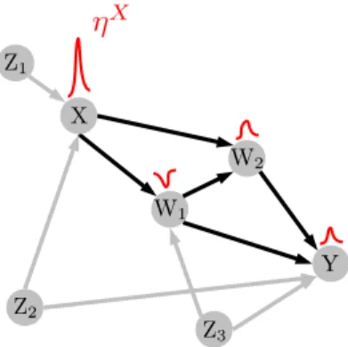
FIG. 1. (Color online) Consider a realization of dynamical noise ηX driving subprocessX as a perturbation. Coupling mechanisms
along different causal paths (black lines) transform such a perturba-tion, and the total effect onYsome time later can also depend on how intermediate processes nonlinearly interact with each other as shown in Sec.V B. The central idea of the momentary information transfer measures presented in this article is to information-theoretically quantify the general effect of such perturbations and isolate it from common drivers in the past such asZ2but alsoZ1and the past ofX. To
also quantify how much intermediate processes such as (W1, W2) on
causal paths mediate information, it will also be important to exclude common drivers likeZ3.
system without dynamical noise, the entropy rate hsymb—
since it is computed by creating a symbol sequence from a coarse graining in phase-space—depends on some resolution parameterr. Then the limit limr→0hsymb might exist and is
called theKolmogorov-Sinai entropy. If this limit is finite and larger than zero, the system is called chaotic. But here we study stochastic, discrete time processes because the finite set of measured variables of a complex system like the Earth will never perfectly describe the full system’s state and all remaining processes contribute to dynamical noise (implying that the Kolmogorov-Sinai entropy diverges).
While the focus in Refs. [36,37] and related works is on decompositions of predictive information on the basis of transfer entropy as an information-theoretic generalization of Granger causality, the concept here is more similar toSims causality, see, e.g., Ref. [47], which takes into account not only direct but also indirect causal effects. Sims causality is based on measuring to what extentXat timethelps in predictingY
at timest> tin the future excluding the past ofXand also the present of all other processes, i.e.,X−t+1=(Xt,Xt−1, . . .). In
model (1) excluding the past essentially isolates the dynamical noise ηX
t and our goal is now to quantify the information transfer emanating fromηX
t into the future (Fig.1).
With this central idea we define two pairs of measures for two purposes: (1) to quantify the information transfer between two causally linked processes and along causal paths and (2) the mediation of intermediate processes. For each of these tasks we define two measures quantifying different notions of information transfer: Both have in common the above idea to extract information originating in process X only at the lagged time t−τ and are conditioned in order to measure only information transfer along causal paths. These measures, thus, complement alternative decomposition approaches such as in Refs. [36,37,39]. The second measure further attempts
to exclude the influence of other drivers ofY or intermediate path nodes to isolate the whole causal information pathway and fulfill a generalized property of coupling strength autonomy as proposed in previous work [48]. In the present context the property of coupling strength autonomy demands that the measure should be uniquely determined by the interaction of the two processes,XandY in the previous example, and possibly intermediate other processesWalone and in a way au-tonomous of how these are driven by the remaining processes. To understand this, consider a simple example: Suppose we have two interacting processesXandY and a third processZ
that drives both of them. Then a bivariate measure of coupling strength between X and Y such as MI will be influenced by the common input of Z, while our demand is that the measure should be autonomous of the interactions ofXandY
withZ.
In summary, this paper generalizes the idea underlying Ref. [48] to use the reconstructed causal network for quantifying general causal interactions. This framework is called the TIGRAMITE approach (time-series graph-based measures of information transfer), which is also the abbreviation of the accompanying software package (available on the author’s website).
Pearl [19] defines the causal effect of X on Y by the hypothetical intervention ofexperimentally settinga variable
Xto a certain valuex. Then thepostinterventionaldistribution
P(Y =y|do(X=x)), which involves the do-operator and is not the same as the conditional distribution, is used to assess whether and in what wayX affects Y. As mentioned before, however, we assume a nonmanipulable complex system and therefore study a weaker notion of causality. From observational data alone, causal effects can only be estimated (oridentified) under certain assumptions about the underlying process and the kind of interventions [19,49]. In Sec.VI Awe discuss Pearl’s causal effect for linear models.
II. INFORMATION-THEORETIC PRELIMINARIES A. Conditional mutual information
The most important information-theoretic measure on which the quantities discussed in this article are based is the conditional mutual information(CMI) given by
I(X;Y|Z)=H(Y|Z)−H(Y|X,Z) =H(X|Z)−H(X|Y,Z), (2) = p(z)
p(x,y|z) log p(x,y|z)
p(x|z)p(y|z)dxdydz, (3) with Shannon’s entropy H [43,44] as a measure of the uncertainty about outcomes of a process. Mutual information (MI), on the other hand, is a measure of the reduction of this uncertainty if another process is measured and CMI can be phrased as the MI between X and Y that is not contained in a third variable Z. Here we use the natural logarithm to measure CMI and derived measures in nats. Note thatX,Y, andZcan also be vectors. Just like MI, CMI is non-negative (which can be shown using Jensen’s inequality [4] and holds for the continuous as well as the discrete case) and symmetric in its first two arguments I(X;Y|Z)=I(Y;X|Z). Further,
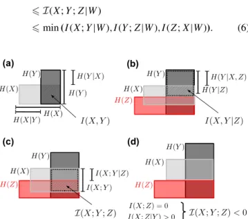
according to Eq. (3), CMI measures the Kullback-Leibler distance [4,50] between the distributions p(x,y|z) and the distribution for the independent casep(x|z)p(y|z) and is zero if and only ifXandYare independentconditionally onZ. This property makes CMI especially useful to measure conditional independence as needed in the definition and estimation of causal graphs (Sec.III). Figures2(a)and2(b)visualize MI and CMI in Venn diagrams as a difference of conditional entropies. In this representation also the symmetry in the arguments is obvious.
B. Interaction information
Just like MI and CMI are differences of conditional entropies, also the difference of CMIs has an interesting interpretation that we will utilize to measure the effect of one random variable on the interaction between two others. Such a measure has been studied in Refs. [51–53] under the name multiple information. We use the terminteraction information with the symbolI, which is symmetrically defined as
I(X;Y;Z)=I(X;Y)−I(X;Y|Z) =I(Y;Z)−I(Y;Z|X)
=I(Z;X)−I(Z;X|Y). (4) In Refs. [54,55] this quantity is defined with the signs reversed, but the above definition is more consistent with the definition of CMI in Eq. (2). It is also straightforward to define theconditional interaction information:
I(X;Y;Z|W)=I(X;Y|W)−I(X;Y|Z,W). (5) Contrary to CMI, the (conditional) interaction information can also be negative and is bounded by
−min(I(X;Y|Z,W),I(Y;Z|X,W),I(Z;X|Y,W))
I(X;Y;Z|W)
min(I(X;Y|W),I(Y;Z|W),I(Z;X|W)). (6)
FIG. 2. (Color online) Venn diagrams of (a) mutual information, (b) conditional mutual information, (c) positive interaction informa-tion, and (d) negative interaction information. The latter case, where the entropies ofXandZdo not “overlap” anymore, demonstrates that the analogy between entropies and sets should not be overinterpreted.
The possible negativity also shows that the visualization in Fig. 2(c) as sets in Venn diagrams should not be over-interpreted. In Fig. 2(d) a case is shown where X and Z
areunconditionallyindependent, but conditionally dependent, leading to I(X;Z|Y)I(X;Z) and, therefore, a negative interaction information. That this property can actually by intuitively understood will be studied in examples in Sec.V.
C. Estimation of (conditional) mutual information In the examples and applications we use a nearest-neighbor estimator [56,57] that is most suitable for variables taking on a continuous range of values and has much less bias than the commonly used binning estimators. This estimator has as a free parameter the number of nearest-neighbors
k which determines the size of hypercubes around each (high-dimensional) sample point. Small values of k lead to a lower estimation bias but higher variance and vice versa. Note that for an estimation from (multivariate) time-series stationarity is required.
III. TIME-SERIES GRAPHS AND CAUSAL PATHS The here-proposed framework to use the reconstructed causal network for quantifying general causal interactions (TIGRAMITE approach) is based on the concept of time-series graphs and causal paths as defined in the following.
A. Time-series graphs
Atime-series graph[58,59] is a certain type of graphical model [60] for the case of time-ordered data and visualizes the Markovian conditional independence properties of a multivariate time-dependent process, i.e., how the joint density of the multivariate process X(including its lags) factorizes. Figures3(a) and3(b) show examples. Each node in a time-series graph represents a subprocess of a multivariate discrete time process X at a certain time t. Directed links between subprocesses (or nodes)Xt−τandYtforτ >0 are marked by an arrow and defined by
Xt−τ→Yt ⇐⇒I(Xt−τ;Yt|X−t \ {Xt−τ})>0, (7) with infinite pastX−t =(Xt−1,Xt−2, . . .), i.e., if they are not
independent conditionally on the past of the whole process, which implies a lag-specific Granger causality with respect toX. IfY =X we say that the linkXt−τ→Yt represents a coupling or cross-link at lagτ, while forY =Xit represents anautodependency or autolink at lagτ.
Since often also contemporaneous associations are of interest, we also define links betweenXtandYtas in previous works [20,48] by
Xt−Yt ⇐⇒I(Xt;Yt|X−t+1\{Xt,Yt})>0, (8) where also the contemporaneous present Xt\{Xt,Yt} is in-cluded in the condition. Note that stationarity implies that
Xt−τ→YtwheneverXt−τ →Ytfor anytand, correspond-ingly, for contemporaneous links. In Ref. [59] also another version of contemporaneous links is defined, marked by a dashed line:
FIG. 3. (Color online) Time series graphs illustrating the path-based measures of information transfer ITX (a) and MITP (b), and process graph (c, the labels denote the lags). Directed links (Def. 7) are marked by arrows, contemporaneous links (Def. 8) by a solid line. There are three causal directed paths connectingXt−3 andYt (black lines), two of length 2 viaW1,t−2 andW2,t−1 and one of length 3: Xt−3→
W1,t−2→W2,t−1→Yt. The idea of the measure ITX shown in (a) here is to quantify how much of the information entering the system inXt−3,
i.e., the dynamical noiseηX, is transferred along causal paths toY
t by conditioning out the effect of the parents ofPXt−3(solid red boxes), its neighbors involving contemporaneous sidepaths toYt denotedNXYtt−3(dashed red box), and the neighbor’s parentsP(N
Yt
Xt−3) (dotted red boxes). The latter two conditioning sets exclude contemporaneous sidepaths likeXt−3−W1,t−3 →W2,t−2 →Yt−1 →Yt. ITX still depends
on processes affecting intermediate nodes on causal paths, e.g., processZ3which drivesW1andY. The idea of MITP shown in (b) now is to
go one step further and isolate all causal paths from the remaining process by additionally conditioning on the parents of the intermediate path nodesCXt−τ→Yt\{Xt−τ}(dashed blue boxes) andY (solid blue boxes). This also allows to isolate mediated effects using momentary interaction
information as defined in Sec.IV C.
In the case of a multivariate autoregressive process, the latter definition corresponds to nonzero entries in the covari-ance matrix of the innovations, while the former corresponds to nonzero entries in the inverse covariance matrix [59]. One problem with Definition (8) is that it can potentially cause spurious links if, e.g., Xt and Yt are independent (also of the past), but both causally drive another process
Zt instantaneously, i.e., at the same timet, which might not be resolved due to a too-coarse time sampling interval. Then
I(Xt;Yt)=0, butI(Xt;Yt|Zt)>0 due to the “conditioning on a common child” effect, see, e.g., Ref. [61], which is shown in Fig.2(d). In this work, we are not considering instantaneous causal effects, but to circumvent this problem in practice, one can consider contemporaneous effects only if both Definitions (9) and (8) are satisfied. Note that both definitions result in slight differences in the definition of open and blocked paths through contemporaneous links as discussed further below.
In Refs. [20,62] a consistent algorithm for the estimation of the above-defined time-series graphs by iteratively inferring the parents and, in a second step, also the neighbors is discussed. This challenging problem is not further addressed here and involves demands such as consistency (i.e., that
the algorithm converges to the true graph for infinite sample sizes), statistical power, underlying assumptions (e.g., faith-fulness [18]), or computational complexity (partly addressed in Ref. [63]).
B. Causal paths
The measures introduced in Sec. IV are CMIs based on paths and different sets of conditions which we determine from the sets of parents and neighbors of a nodeYt defined, respectively, as
PYt = {Zt−τ:Z∈X,τ >0,Zt−τ →Yt}, (10) NYt = {Xt :X∈X,Xt−Yt}. (11) Our main interest lies in causal paths in the time-series graph which are defined as directed paths, i.e., containing only motifs→ • →(assuming that the arrow of time in the time-series graph goes to the right). But there are also other paths on which information is shared even though no causal interventions could “travel” along these. In general [59], in the above-defined time-series graph with solid contemporaneous
links a path between two nodesu andv is calledopen if it contains only the motifs→ • →,← • →,− • →, or− • −. On the other hand, if any motif on a path is→ • ←or→ • −, the path is blocked. Nodes in such motifs are also called colliders. If we now consider a separating or conditioning setS, then openness and blockedness of conditioned motifs reverse, i.e., denoting a conditioned node by, the motifs → →, ← →, − →, and −− are blocked and the motifs→ ←and→−become open. Note that for the alternative definition of contemporaneous links Eq. (9) marked with dashed lines, the motif - - -• - - - is blocked while the conditioned motif - - -- - - is open.
Two nodes u and v are separated given a set S if all paths between the two are blocked. Conversely, two nodes are connected given a setS if at least one path between the two is open. The Markov property, which we assume throughout, now relates separation in the time-series graph to conditional independence relations in the underlying process which can be quantified with CMI (as a conditional independence measure):
uandvseparated givenS⇒I(u;v|S)=0. (12) The path-based CMIs are constructed with conditions to block all noncausal paths and only leave open causal paths. In particular, alsocontemporaneous sidepaths, which start with one or more contemporaneous links followed by a directed path
u− • − · · · − • → · · · →v, need to be blocked. Note that we do not consider contemporaneous causal effects here which might occur due to a too-low sampling rate of the process.
IV. TIME-SERIES GRAPH-BASED MEASURES OF INFORMATION TRANSFER (TIGRAMITE APPROACH)
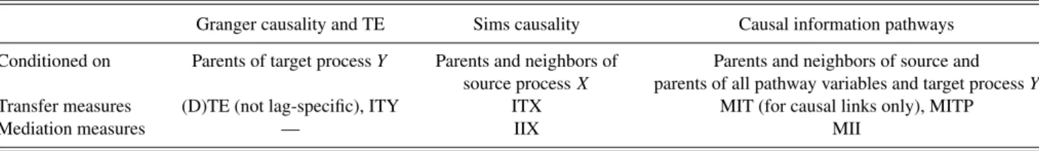
In the following we briefly discuss the transfer entropy ansatz to measuring information transfer and introduce our novel approach to quantify different aspects of information transfer through causal links and paths. Table I provides an overview over these different classes of measures. As mentioned in the Introduction, the proposed measures of information transfer are CMIs based on different sets of conditions which we determine from the reconstructed time-series graph. The TIGRAMITE approach has the advantage of a low-dimensional estimation problem without arbitrary truncation parameters like in the original definition of transfer entropy involving infinite vectors.
A. Transfer entropy ansatz
Transfer entropy (TE), introduced by Schreiber [64], is the information-theoretic analog of Granger causality and
for multivariate Gaussian processes they can be shown to be equivalent [65]. The key idea to arrive at a causal notion of information transfer is to measure the information content of the past of a processXat timest< tabout the target variable
Y at timetand exclude information from the common history shared byXandY. In its multivariate version, TE is defined as
IXTE→Y =I(Xt−;Yt|X−t \X−t ). (13) TE measures the aggregated influence of X at all past lags, i.e., it is not lag specific, and leads to the problem that infinite-dimensional densities have to be estimated, which is commonly called the “curse of dimensionality.” In Ref. [20] this problem is overcome by a decomposition formula. In practice, however, a truncated version at some maximal delay is typically used. In Ref. [48] a lag-specific variant of TE taking into account the time-series graph structure was introduced, called theinformation transfer to Y(ITY) defined as
IXITY→Y(τ)=IXt−τ;YtPYt\{Xt−τ}
. (14) ITY differs from a bivariate lag-specific TE definition such as in Ref. [66] since it explicitly uses the previously reconstructed parentsPYt ⊂X−, which includes drivers from the past of the whole process and not onlyY’s own past.
TE can be derived as one component of decomposing the prediction entropyI(X−t ;Yt) [36]. A similar approach is developed in Ref. [37]. The decisive difference of these transfer entropy related measures to our proposed framework is that they measure the contribution of different drivers to predicting a target variable Y, i.e., they are aimed at decomposing the predictive information. In particular, Granger causality, TE, or ITY are zero for indirect causal interactions, i.e., if the interaction is mediated via another measured process. With respect to time-series graphs, ITY is one way to quantify the strength of a causal coupling link betweenXandY at some lagτ. For a detailed account on the interpretability of different measures of the strength of causal links see Ref. [48].
B. Quantifying information transfer along paths In this article the main question of interest is not only how strong a causal link is but, more generally, how strong an indirect causal influence of a variableXt−τ onYt is (Fig.3). Indirect causal effects can only be transferred oncausal paths in the time-series graph, which are paths consisting only of directed links as defined in Sec. III B. Note that Fig. 3(c)
shows an aggregated process graph, which is not suited to read off causal paths since it does not show the full spatiotemporal TABLE I. Three different types of time-series graph-based measures of information transfer (TIGRAMITE approach). Transfer measures refer to CMI-based quantities to measure information transfer between two variables and mediation measures to the interaction information-based quantities between multiple variables. Decomposed transfer entropy (DTE) was introduced in Ref. [20].
Granger causality and TE Sims causality Causal information pathways Conditioned on Parents of target processY Parents and neighbors of Parents and neighbors of source and
source processX parents of all pathway variables and target processY
Transfer measures (D)TE (not lag-specific), ITY ITX MIT (for causal links only), MITP
causal structure (including autodependencies) like time-series graphs.
We denote the processes along causal paths includingXt−τ forτ >0 and excludingYt by
CXt−τ→Yt = {Xt−τ} ∪ Wt−τW ∈X − t withτ > τW >0 : Xt−τ →. . .→Wt−τW →. . .→Yt , (15) where→. . .→denotes a succession of directed links or only one directed link. These can be read off directly from the time-series graph. For example, in Fig. 3, Xt−3 and Yt are connected by the three causal paths Xt−3→W2,t−1→Yt,
Xt−3→W1,t−2→Yt, and Xt−3→W1,t−2 →W2,t−1→Yt such thatCXt−3→Yt = {Xt−3, W1,t−2, W2,t−1}. Our goal is now to construct a CMI with conditions that leave open only these causal paths and block all noncausal paths according to the definition of paths and blocking in time-series graphs in Sec.III B.
The first step is to exclude paths due to common drivers ofX
andY. The parentsPXt−τ ofXat timet−τblock all common drivers from the past since these paths necessarily contain the motifs − • →Xt−τ or → • →Xt−τ, which are both blocked if conditioned on. A second class of noncausal paths are contemporaneous sidepaths as defined in Sec.III B. These can be blocked by conditioning on those contemporaneous neighbors of Xt−τ that have at least one contemporaneous sidepath, of coursenot traversingXt−τ, which we define as
NYt
Xt−τ = {Wt−τ ∈NXt−τ :Xt−τ−Wt−τ→− . . .→Yt}, (16) where→− . . .→denotes either a directed path or a contem-poraneous sidepath that does not involveXt−τ. For example, in Figs.3(a)and3(b),NYt
Xt−3 = {W1,t−3}. On the other hand, for the causal pathXt−2→Xt−1→Xt we haveN
Xt Xt−2= ∅, since there are no contemporaneous sidepaths from W1,t−2
toXt. The condition on neighbors unfortunately introduces new open paths becauseXt−τ−← is an open motif. To block these paths, one needs to additionally condition on the parents of the neighborsP(NYt
Xt−τ). Note that one could also only select those parents fromXt−τ which have a “common driver path” toYt, but our goal is to isolate the momentary informationentering the system inX, i.e., the dynamical noise from model (1), and quantify its propagation along causal paths toY some time later. Theinformation transfer fromX(ITX) is now defined forτ >0 as
IXITX t−τ→Yt =I Xt−τ;YtPXt−τ,N Yt Xt−τ,P NYt Xt−τ . (17) It measures the part of source entropy in Xt−τ that reachesYt on any causal path and could be regarded as an information-theoretic analog to Sims causality as mentioned in the introduction (see also TableI). In Ref. [48] this measure was introduced without the condition on neighbors.
ITX does not exclude information entering processYtfrom other sources, for example, from processZ3 in the example shown in Fig. 3(a). The idea of momentary information transfer [48] was to isolate the information shared between two processes via a causal link from the remaining process. Now this idea can be generalized by isolating all causal paths from the remaining process to assess the part of the source entropy
ofXt−τthat is transferred on any causal path and shared with
Yt, excluding the parents of all intermediate path nodes and
Y that are not part of the causal path. Figure3(b)illustrates this idea. With the nodes on all causal paths includingXt−τ denoted by CXt−τ→Yt [Eq. (15)], themomentary information transfer along causal paths(MITP) is defined as
IXMITP→Y(τ)=IXt−τ;YtPYt\CXt−τ→Yt,P(CXt−τ→Yt), NYt Xt−τ,P NYt Xt−τ . (18) For the time-series graph example in Fig. 3(b), these conditions are marked by the red and blue boxes. In Sec.V
we will prove that MITP, contrary to ITX, also fulfills a generalized coupling strength autonomy theorem which allows us to better relate it to the underlying dynamics of a process as will be discussed in Sec.VI.
If CXt−τ→Yt = {Xt−τ} and under the “no sidepath”-constraint in Ref. [48], the conditions on the neighbors can be dropped and MITP collapses to MIT.
C. Quantifying mediating information transfer Looking at Fig.3, one immediate question is whether one can quantify how much of the information transfer between
X and Y went through W1 and how much through W2. Which of these is information-theoretically more important for explaining the indirect causal relationship betweenXand
Y? The interaction information defined in Eq. (4) can be used to answer this question, and we here discuss two analogous versions for the measures ITX and MITP. For two processes
Xt−τandYtconnected by a causal path, intermediate processes can occur with multiple lags. For example, among the causal paths betweenXt−4andYtin Fig.3, the processW1is traversed
at lags W1,t−2 andW1,t−3. Generally, if a subprocess W is
intermediate in an interaction Xt−τ → · · · →Yt at multiple lags t−τ1, t−τ2, . . ., we here include all these lags in the vectorW= {Wt−τ1,Wt−τ2, . . .} ⊂CXt−τ→Yt.
First, we define theinteraction information from X(IIX) as IIIX Xt−τ→Yt|W=I Xt−τ;Yt;WPXt−τ,N Yt Xt−τ,P NYt Xt−τ (19) = IXITX→Y(τ)−IXt−τ;YtPXt−τ,N Yt Xt−τ,P NYt Xt−τ ,W ITX conditioned onW . (20) IIX measures the effect of an intermediate processWon the information transfer between the source information ofXt−τ andYt. Second, themomentary interaction information(MII) for an intermediate processWis defined as
IMII X→Y|W(τ)=I Xt−τ;Yt;WPYt\CXt−τ→Yt,P CXt−τ→Yt , NYt Xt−τ,P NYt Xt−τ (21) =IXMITP→Y(τ)−IXt−τ;YtPYt\CXt−τ→Yt,P CXt−τ→Yt , NYt Xt−τ,P NYt Xt−τ ,W MITP conditioned onW . (22)
MII measures the effect ofWon the momentary informa-tion transfer along paths betweenXt−τandYtand additionally
isolates the influence of drivers of the causal path processes. In Sec. V we discuss several examples demonstrating that IIX and MII are not necessarily always positive, implying that an intermediate process can counteract the interaction betweenXt−τandYt. This measure can naturally be extended by including sets of processes from CXt−τ→Yt. Due to the symmetry of interaction information as defined in Eq. (4), MII is symmetric in its arguments excluding the condition.
Table I provides an overview over the different classes of measures discussed here. In a climate data example in Sec.VII, we will see how IIX and MII can be used to quantify dominant pathway mechanisms and in Sec.VI Cwe discuss how they can be used as an aggregate measure of “causal interaction betweenness,” modifying concepts from complex network theory for functional network analysis [1].
V. EXAMPLES AND THEOREMS
In the following we discuss how the novel approach allows to extract a detailed picture of interaction mechanisms between multiple processes.
A. Linear model example
In Ref. [48] the strength of direct causal links was studied. The main finding was that MIT solely depends on the coefficient corresponding to the causal link. This property was calledcoupling strength autonomy in Ref. [48] and will be reviewed in Sec.V C. For the case of interactions along causal paths, consider the following linear model with time-series graph visualized in Fig.4(a):
Xt=αXt−1+ηXt
Wt=αWt−1+aXt−1+ηWt (23)
Yt=αYt−1+cXt−2+bWt−1+ηYt,
where all processes are jointly zero-mean Gaussian with vari-ancesσX2, σY2, σZ2of the innovation termsη·. Here the influence ofXt−2onYt has two paths: one via the direct coupling link
Xt−2→Ytand one via the pathXt−2→Wt−1→Ytsuch that we can rewrite Yt=cXt−2+b aXt−2+ηtW−1 +ηtY, (24) from which we see that the coupling cannot be unambiguously related to one coefficient and interesting dynamics emerge. In Fig.4(b)we investigate the measures ITX, MITP, IIX, and MII numerically for varyinga=b(strength of the sidepath) and
c(strength of direct link) for fixed autodependency strength
α=0.5. We assumea,b=0, because otherwise this causal path vanishes and IIX or MII are not defined. The ensemble size to estimate the ensemble mean is 30, the sample length isT =
10 000, and the CMI nearest-neighbor estimation parameter is
k=1 to achieve minimal bias [57]. As mentioned in Sec.II C, for largerkthe bias increases, but also the estimator’s variance decreases.
Since we varya together withb, the contribution via this sidepath is always positive, for positive and negativea, b. Ifc
is also positive, we observe an increase in ITX as well as MITP [Fig.4(b)], with the latter being more pronounced. For negative
c, on the other hand, the contributions of the direct link and
the sidepathcounteractand, for certain values, (a, b, c) even cancel out, leading to a vanishing ITX and MITP.
These different types of mediation of the intermediate process W can be quantified by IIX and MII [lower panels in Fig.4(b)]: For positivec, both are larger than zero, showing the positive contribution of both mechanisms; also here MII is more pronounced. Forc=0, MII is equal to MITP because the only interaction stems from the causal path demonstrating the explanatory influence ofW, which acts as the only mediating process. In the Venn diagram of Fig. 2(c) this corresponds to the case in which H(W) entails all of the shared entropy betweenXandY. For negativec, the counteracting effect is evident in the negative sign of IIX and MII which implies for the latter thatIXMII→Y|W(τ =2)> IXMITP→Y(τ =2): Conditioning out the effect of the intermediate processW here reveals that the direct link is actually very strong and was only “masked” by the counteracting sidepath viaW. In Ref. [37] a similar case, but without isolating the interaction pathway, was termed a “synergistic” contribution to the predictive information about
Yas opposed to the “redundant” case with a positive interaction information.
In Fig.4(c)the dependence of the four measures fora= b=0.5 and varying the autodependency strengthαand direct link strength cis shown. ITX features a strong dependency onαalready for weak drivingsα≈0.4 and almost vanishes for a very strong driving. Note that the same effect would be observed if other external processes driveW andY (fromX
the effect is partially excluded due to the condition on PX). Analytically, here ITX can only be reduced to
IXITX→Y(τ =2) = I(Xt−2;Yt|Xt−3)
= IαXt−3+ηtX−2;Yt|Xt−3
Eq. (A6) in Appendix
= IηXt−2;Yt|Xt−3
, (25)
which still depends on many coefficients in the model and cannot be easily related to the underlying dynamics. On the other hand, MITP can be simply related to the coefficients along the causal paths as
IXMITP→Y(τ =2)=1 2ln 1+(c+ab) 2σ2 X b2σ2 W +σY2 , (26)
which follows from Theorem 2 in Sec.V C. Here it becomes evident that MITP vanishes along the parabola c= −a b
(which can be considered a pathological case where the causal assumption offaithfulnessis violated [18]). A second impor-tant finding is that MITP isindependentof the autodependency coefficientα. The same holds for MII, here given by
IMII X→Y|W = 1 2ln 1+(c+ab) 2σ2 X b2σ2 W+σY2 −1 2ln 1+ c 2σ2 XσW2 σW2 +a2σ2 X σY2 , (27)
FIG. 4. (Color online) (a) Time-series graph for model (23) of a causal interaction between three processes at different lags (black dots). The parents are shown in colored boxes, here there are no neighbors.a, b, c, αdenote the model coefficients. In (b) the interaction measures are plotted againsta=b(strength of the sidepath) andc(strength of direct link) for an autodependency strengthα=0.5, and in (c) against cand the autodependency strengthαfora=b=0.5. The color shading only emphasizes the sign and strength, the value can be read off thez-axis. All innovation termsηhave unit variance. Further parameters: ensemble size 30, sample lengthT =10,000, nearest-neighbor estimation parameterk=1.
FIG. 5. (Color online) Same as in Fig.4but for the nonlinear model (28). as follows from (A4) in the Appendix. This implies that the
value of MITP and MII can solely be related to the model’s coefficients along the causal interaction paths, which can be considered an advantage in interpreting these measures compared to ITX or IIX. While in this example there are no external parents influencing the processes along the path, in more complex schemes also their effect can be excluded by the condition on the parents of the nodes on the path denoted byCXt−τ→Yt. In Sec. 3 this will be proven for the general case. Note that in Fig.4(c)MITP and MII are slightly affected for very strong autodependencies which is due to an estimation bias and vanishes for infinite sample sizes. This model will be further discussed in relation to linear causal effect measures in Sec.VI A.
B. Nonlinear model example
Next we discuss a nonlinear version of model (23) which shares the same time-series graph but features different
dynamics: Xt =αXt−1+ηtX Wt =αWt−1+aXt−1+ηWt (28) Yt =αYt−1+ cbXt−2Wt−1 multiplicative dependency +ηtY,
with Gaussian innovation terms as before. Figure5(a)shows that ITX and MITP vanish forb or c equal to zero and are increasing for larger absolute values. For larger|c|and certain values ofa,bwe observe a counteracting of W through the indirect path as can be seen from the negative IIX and MII, but no annihilation of both effects occurs here and ITX and MITP stay positive. For this nonlinear dependency structure both ITX and MITP (and the corresponding interaction informations) depend on the external forcing parameter α [Fig. 5(b)]. The reason is that the nonlinearity mixes the terms and the
dependencies cannot be conditioned out anymore. Consider model (28) but with differing autodependency termsα, β, γ
forX, W, Y, respectively. MITP here is given by
IXMITP→Y(τ =2) = I(Xt−2;Yt|Xt−3, Wt−2, Yt−1) Eq. (A6)
= IηXt−2;Yt|Xt−3, Wt−2, Yt−1
, (29) and the dependency ofYt can be rewritten as
Yt=cb aηXt−2+ηtW−1ηXt−2+ηYt + cbαaXt−3ηXt−2+αXt−3ηtW−1 + βWt−2ηXt−2+αaXt−3ηXt−2 + γ Yt−1+cb αβXt−3Wt−2+aα2X2t−3 . (30) Here in MITP the last line vanishes due to the condition on (Xt−3, Wt−2, Yt−1), but due to the multiplicative mixing
with the noise terms in the second and third line, the autodependency coefficientsα, β (but not γ) still determine MITP. ITX additionally depends on γ. This model, there-fore, demonstrates a case where “external effects” cannot be excluded anymore. Thus, while the information-theoretic interpretation still holds, MITP cannot be easily related to the system’s dynamics. Still, plots like in Figs.4and5can help to better understand dynamical interactions also in toy models from nonlinear dynamics. In the next section we prove under which general assumptions the coupling strength autonomy holds for MITP and MII. The multiplicative dependency can be seen as an example of synergy which has recently gained a lot of interest in information-theoretical studies, see, e.g., Refs. [67,68]. In Ref. [63] synergistic effects are studied with respect to optimal prediction schemes.
C. Theorems
In this section we state some inequality relations among the novel measures and generalize the coupling strength autonomy theorem for MIT [48] to the path-based measures MITP and MII.
Theorem 1(Inequality relations). Forτ >0, the following inequalities hold: IIIX X→Y|W(τ)I ITX X→Y(τ), (31) IMII X→Y|W(τ)IXMITP→Y(τ), (32) IXITX→Y(τ)IXMITP→Y(τ). (33) The first two inequalities are trivially fulfilled since IIX and MII are defined by ITX and MITPminusa CMI, which is always positive. Equality holds if the intermediate node(s) Wexplain the entire interaction betweenX andY. The last inequality is proven in AppendixA1.
In practice, this inequality is often not fulfilled because the estimation dimension of MITP is typically much larger than that of ITX and finite sample effects lead to a negative bias which often leads to MITP being smaller than ITX. This also makes a comparison of the values of ITX and MITP more difficult.
To generalize the coupling strength autonomy theorem from MIT to MITP and MII, we consider causal paths as defined
in Sec. III B instead of only causal links. While the careful condition on only those neighbors that have sidepaths excludes dependencies of MITP and MII on the dynamics along these sidepaths, one cannot avoid a contemporaneous dependency on the interaction with the respective neighbor itself. This also holds for other intermediate processes on causal paths. For the following theorems, we define as a “no contemporaneous dependency” condition ∀Wt(−i)τ i ∈CXt−τ→Yt : N Yt Wt(i)−τi = ∅ (34) withNYt Wt(i)−τi
defined in Eq. (16). This condition implies that no contemporaneous sidepaths as defined in Sec.III B emanate from any of the path nodesCXt−τ→Yt (includingXt−τ) towards
Yt. Note that we denote byW( i)
t−τi each individual subprocess along causal paths at a certain lagτi. If one subprocess occurs at multiple lags, it will have another indexifor each lag.
Theorem 2(Coupling strength autonomy for MITP). Let
X, Ybe two subprocesses of a multivariate stationary discrete-time processXsufficing the Markov property [Eq. (12)] with time-series graphG. We assume thatXt−τandYtare connected by a directed path with path nodesCXt−τ→Yt includingXt−τas defined in Eq. (15). We denote those parents ofYt that are in the path nodes asPYC=PYt ∩CXt−τ→Yt and correspondingly for other path nodes and assume the following dependencies:
Xt =gX PXt−τ +ηXt (35) Yt =fY PC Y +gY PYt \P C Y +ηYt,
wherefYis linear andgX,Yarbitrary. Further, for all path nodes
W(i)we assume the dependencies
Wt(i)=fi PC i +gi Pi\PiC +ηit (36) ∀W(i)∈CXt−τ→Yt \ {Xt−τ},
where thefiare again linear, thegiare arbitrary functions and the dynamical noise termsη·are independent and identically distribuited due to Markovity. Then MITP [Eq. (18)] is given by IXMITP→Y(τ)=IηtX−τ;ηtY+fηtX−τ,∪iηit−τi PY t\CXt−τ→Yt,P CXt−τ→Yt ,NYt Xt−τ,P NYt Xt−τ , (37) where 0< τi < τ∀i. If, further, the “no contemporaneous dependency” condition (34) holds, then MITP reduces to a mutual information
IXMITP→Y(τ)=IηtX−τ;ηtY+fηtX−τ,∪iηit−τi
, (38) wheref is a linear function and∪iηi denotes the innovation terms or dynamical noise of all path nodes in CXt−τ→Yt \ {Xt−τ}.
The proof is given in Appendix (A3). This theorem also includes the coupling strength autonomy theorem for MIT [48] as a special case if CXt−τ→Yt = {Xt−τ} and under the “no sidepath” constraint in Ref. [48], thenf(ηX
t−τ,∪iηti−τi)=
f(ηX t−τ).
Since momentary interaction information (MII) is the difference between MITP and the MITP conditioned on one
of the path nodes (excludingXt−τ), the theorem follows from the above theorem.
Theorem 3(Coupling strength autonomy for MII). Using the same assumptions as for Theorem 2, the momentary interaction information IMII
X→Y|W(τ) between Xt−τ, Yt and one or more intermediate processesW=(Wt(1)−τ1, Wt(2)−τ2 . . .)∈ CXt−τ→Yt \ {Xt−τ}indexed byj reduces to IηtX−τ;ηtY+fηtX−τ,∪iηit−τi ; ηjt−τj +fj ηtX−τ,∪i=j ηit−τi j PYt\CXt−τ→Yt,P CXt−τ→Yt ,NYt Xt−τ,P NYt Xt−τ , (39)
and, if, further, the “no contemporaneous dependency” condi-tion (34) holds, to IηXt−τ;ηYt +f(ηXt−τ,∪iηti−τi); ηjt−τj +fj ηtX−τ,∪i=j ηit−τi j , (40)
for linear functionsf, fj.
The proof is given in (A4) in the Appendix. For the case of a causal triple as shown in Fig.4this further reduces to
IηXt−τ;ηYt +(c+ab)ηXt−τ+bηWt−τW;ηtW−τW +aηXt−τ, (41) from which the special case with Gaussian innovations Eq. (27) follows.
VI. DISCUSSION
A. Relation to linear causal effect theory
We phrased the idea of causal influence in an information-theoretic setting. Pearl’s theory of causal effects [19,21] can also be embedded in the time-series graph framework [49]. Assuming the time-series graph is causally sufficient [19] and all dependencies are linear, causal effects can simply by derived from multivariate regressions. First, analogously to ITY or MIT as a measure of direct link strength, the path coefficient of a link is given by the corresponding (typically standardized) coefficient in a multivariate regression of each process on its parents in the time-series graph [69]. Further, analogously to ITX or MITP, the linear causal effect of Xt−τ on Yt also via indirect paths can be estimated by a standardized regression of Y on the multiple regressors {Xt−τ,P(Xt−τ)}. The linear causal effect (CE) [19,21] is then given by the corresponding (standardized) regression coefficientrbelonging toXt−τ,
rXCE→Y(τ)=rYtXt−τ·P(Xt−τ). (42)
This formulation assumes the “no contemporaneous depen-dency” condition (34) for simplicity, but it can be generalized. The causal effectrXCE→Y(τ) quantifies the change in the expecta-tion ofYt(in units of its standard deviation) induced by raising the laggedXt−τ by one standard deviation, while keeping the parents ofXt−τconstant. Then the total causal effect between lagged processes is simply given by the sum over the product of path coefficients along each causal paths connectingXt−τ andYt. For example, for the model (23) with time-series graph in Fig.4(a)the total linear causal effect betweenXt−2andYt is given by
X
Y(c+ab), where the square root contains the normalization by the variances which, however, depends on the autodependency strength and other coefficients here. ITX is simply the mutual information with the same conditions as CE (if no neighbors are present), while MITP for this model example [see Eq. (38) or Eq. (26)] is12ln [1+(c+ab)2σX2
b2σ2 W+σY2]. ITX, MITP, and CE all depend on the “coupling mechanism” (c+ab), but with different “normalizations.”
Even in linear models, themediated causal effect(MCE) is more difficult to identify [19,70]. The causal interpretation is that an indirect effect via the node(s) W measures the increase we would see inYt while holdingXt−τ and all other intermediate nodes and parents ofXt−τconstant and increasing the node(s)W to whatever value it would obtain under a unit change in Xt−τ while holding the parents ofXt−τ constant [19,70]. To identify MCE for the triplet case in model (23) with time-series graph in Fig.4(a)one can subtract from CE the contribution of all pathsnotpassing throughW:
rXMCE→Y|W(τ =2)=rXCE→Y(2)−rYtXt−2·P(Xt−2),Wt−1,P(Wt−1)
CE excluding paths throughW
=
X
Y
ab . (43)
Note the additional condition on the parents of W here needed to exclude a confounding of the mediating link from
W to Y from the past due to Wt−2. This is also the idea
behind the interaction information MII which is conditioned on the parents of all intermediate processes to exclude possible confounding. MII is given also by a difference, but of CMIs instead of regressions: 1
2ln [1+ (c+ab)2σ2 X b2σ2 W+σY2 ]− 1 2ln [1+ c2σ2 XσW2 (σ2 W+a2σX2)σY2
], where the latter term information-theoretically quantifies the strength of the direct link with coefficient c. The linear framework allows for quantifying the relative influence of paths between two processes by the “locally” estimated weights making it easy to interpret, but it rests on a linear assumption. Another advantage of the linear approach is that total and indirect effects can also be investigated in the frequency domain in the framework of directed transfer functions [25–27]. To some extent causal effects can also be estimated for more general nonlinear structural equation models [19,71], but especially mediated effects are difficult to identify if no strong assumptions are fulfilled [70].