directional sensor networks on smart city
.
White Rose Research Online URL for this paper:
http://eprints.whiterose.ac.uk/150623/
Version: Accepted Version
Article:
Cao, B., Zhao, J., Yang, P. orcid.org/0000-0002-8553-7127 et al. (3 more authors) (2019)
3-D deployment optimization for heterogeneous wireless directional sensor networks on
smart city. IEEE Transactions on Industrial Informatics, 15 (3). pp. 1798-1808. ISSN
1551-3203
https://doi.org/10.1109/tii.2018.2884951
© 2018 IEEE. Personal use of this material is permitted. Permission from IEEE must be
obtained for all other users, including reprinting/ republishing this material for advertising or
promotional purposes, creating new collective works for resale or redistribution to servers
or lists, or reuse of any copyrighted components of this work in other works. Reproduced
in accordance with the publisher's self-archiving policy.
[email protected] https://eprints.whiterose.ac.uk/ Reuse
Items deposited in White Rose Research Online are protected by copyright, with all rights reserved unless indicated otherwise. They may be downloaded and/or printed for private study, or other acts as permitted by national copyright laws. The publisher or other rights holders may allow further reproduction and re-use of the full text version. This is indicated by the licence information on the White Rose Research Online record for the item.
Takedown
If you consider content in White Rose Research Online to be in breach of UK law, please notify us by
Directional Sensor Networks on Smart City.
White Rose Research Online URL for this paper:
http://eprints.whiterose.ac.uk/150623/
Version: Accepted Version
Article:
Cao, B orcid.o
rg/0000-0003-4558-9501, Zhao, J orcid.org/0000-0003-0424-4056, Yang, P
orcid.org/0000-0002-8553-7127 et al. (3 more authors) (2019) 3-D Deployment
Optimization for Heterogeneous Wireless Directional Sensor Networks on Smart City.
IEEE Transactions on Industrial Informatics, 15 (3). pp. 1798-1808. ISSN 1551-3203
https://doi.org/10.1109/tii.2018.2884951
[email protected] https://eprints.whiterose.ac.uk/ Reuse
Items deposited in White Rose Research Online are protected by copyright, with all rights reserved unless indicated otherwise. They may be downloaded and/or printed for private study, or other acts as permitted by national copyright laws. The publisher or other rights holders may allow further reproduction and re-use of the full text version. This is indicated by the licence information on the White Rose Research Online record for the item.
Takedown
If you consider content in White Rose Research Online to be in breach of UK law, please notify us by
3D deployment optimization for
Heterogeneous Wireless Directional Sensor
Networks on Smart City
Abstract—The development of smart cities and the e-mergence of 3D urban terrain data have introduced new requirements and issues to the research of wireless sensor network (WSN) 3D deployment. In this paper, we study the deployment issue of heterogeneous wireless directional sensor networks (HWDSNs) on 3D smart cities. Tradition-ally, studies about the deployment problem of WSNs show solicitude for omni-directional sensors on 2D plane or in 3D full space. As WSNs exist in complex 3D environments and directional sensors are emerging, the work of this paper will have more practical significance. Based on the 3D urban terrain data, we transform the deployment problem into a multiobjective optimization problem (MOP), in which objectives ofCoverage,Connectivity Quality andLifetime, as well as theConnectivityandReliability constraints are simultaneously given close attention to. A graph-based 3D signal propagation model employing the line-of-sight (LOS) concept is used to calculate the signal path loss. The novel distributed parallel multiobjective evolutionary algorithms (MOEAs) are proposed. For verification, a real-world and an artificial urban terrains are utilized. Compared with other state-of-the-art MOEAs, the novel algorithms address the deployment problem more effectively and more efficiently in terms of optimization performance and operation time, respectively.
Index Terms—Wireless sensor network deployment, het-erogeneous wireless directional sensor networks (HWD-SNs), signal propagation model, line-of-sight (LOS), dis-tributed parallelism.
I. INTRODUCTION
W
ITH development of smart cities [1], complex 3D urban environment has brought new problems and challenges to the study of wireless sensor network (WSN) deployment.Many studies have addressed the deployment problem of WSNs. Nevertheless, the majority of them focus on the cov-erage and lifetime of networks [2]–[4] and deploy WSNs on 2D plane or 3D full space. Additionally, the sensors studied are usually omni-directional, which are disk-shaped in 2D and sphere-shaped in 3D, and are based on the deterministic boolean model; that is, within a predefined distance, denoted as Rs, objects can be detected; otherwise, the sensor does not “know” whether there are objects.
Based on the concept of directional sensor networks [5], Teng et al. [6] put forward a fuzzy ring based fan-shaped per-ception model. Sung et al. [7] explored the coverage problem of directional sensor nodes utilizing the concept of Voronoi diagram. Actually, the sensing ability of a sensor will gradually decrease with the increment of distance (omni-directional and
directional sensors) and angle (directional sensors). In the works of [8] and [9], two probabilistic sensing models, using various mathematical formulae to simulate the sensing behav-ior of sensors, were proposed, which better suited real-world applications. Also, traditionally, in the WSNs, the sensors are of the same type and the WSNs are homogeneous. However, heterogeneous WSNs comprised of different types of sensors or sensors with different sensing abilities are more practical. The work of [1] pointed out that the WSNs in the smart cities would be heterogeneous [10]. Based on the work of [11], we will consider heterogeneous directional sensor networks.
The deep integration between information and communi-cation technology (ICT) calls for more network performance [12], in order to achieve the data transmission stability in Internet of Things (IoT) [13], a stable and reliable network is essential [12]. In the smart cities, wireless networks should be stable and reliable in real-time supervisory, data acquisi-tion and communicaacquisi-tion because of the complex, hard and uncontrollable situation. In the smart cities, there are critical offers such as high temperatures, noise, and climate changes [14], the data transmission will be affected by the interference and the abrupt of link because of these changing environment, which require strong connection and reliability. Connectivity is basic for the reliable data transmission, also important for the topology control and routing protocol. Node’s position change affects not only the network lifetime, but also the connection, communication and reliability. Besides the basic coverage and lifetime, connection and reliability [15] also could be con-cerned to ensure the wireless networks performance, specially in the complex environment.
The way of node clustering and routing [16] greatly influ-ences the network performance. Halder et al. [17] discovered that the energy imbalance across the network mainly owing to the data transmission to relay nodes from different sections of the network and put forward a heterogeneous node deployment strategy to deploy sensor nodes and relay nodes to extend network lifetime. While Chu et al. [18] considered the energy consumption rates of different nodes, the residual energy of each node, the communication costs among nodes and the cooperation of different nodes (even some nodes increased energy consumption to assist other nodes in reducing energy consumption), proposing a distributed cooperative topology control. Hacioglu et al. [19] presented a clustering-based routing methodology, which minimized the communication costs among clusters and maximized the node quantity in each cluster, and nondominated sorting genetic algorithm II (NSGA-II) [20] was combined to select excellent solutions.
However, all these studies only explored the case of 2D plane.
Wang et al. [21] utilized particle swarm optimization (P-SO) algorithm [22] to optimize the deployment of WSNs in the industrial environment, and the network reliability was guaranteed by associating each sensor node and each relay node with several relay nodes. Al-Turjman et al. [23] [24] conducted deployment optimization of relay nodes in the 3D space, and the network lifetime and reliability were concerned. Alexandris [25] discussed the connectivity of the networks with communication link. Shu et al. [26] discussed the way of prolonging the connectivity of WSNs.
Additionally, according to the real-world 3D urban terrain data, we know that the terrain may be uneven, and obstacles (e.g., buildings) may exist. The 2D plane situation is too simple to accurately simulate practical situations. Akbarzadeh et al. [8], Topcuoglu et al. [27] and Temel et al. [28] studied the deployment problem on 3D terrain. Omni-directional sensors were considered in [28], while [8] and [27] studied directional sensors. Because of the unevenness of the 3D terrain, the concept of line-of-sight (LOS) [29] was employed in the above works. Moreover, only one objective (i.e., coverage) was studied in [8] and [28]; the stealth and cost of WSNs were also considered in [27], however, all three objectives were transformed to one value on the basis of multiattribute utility theory. Unlike the above three works, Cao et al. [11] de-ployed heterogeneous directional sensors on 3D terrains (plain, hill and mountain), considered multiple objectives (coverage, connectivity uniformity and deployment cost) and utilized multiobjective evolutionary algorithms (MOEAs) to optimize them simultaneously; however, no buildings were taken into account, thus, the node positions were not constrained.
Compared to wired communication, there is no need to arrange and maintain cables for wireless communication; however, the communication range is limited.Usually, for the connectivity of WSNs, the communication range of sensor nodes is simply assumed to be twice the length of the sensing distance, and the full coverage of the target area indicates the connectivity of the WSNs. However, this simplification is unsuitable for real-world applications. Generally, the wireless signal can be reflected, scattered and diffracted and will dis-sipate along the transmission path. Traditionally, to calculate the signal intensity at a given point, from the transmitter, a large number of signal rays are simulated. The accumulation of signal rays at a given point becomes its signal intensity. He et al. [30], [31] utilized the ray-tracing method based on image concept, which was more computationally efficient.
Unlike other works, the contributions of this paper can be summarized as follows:
1) The deployment problem of heterogeneous wireless di-rectional sensor networks (HWDSNs), including sensor nodes with various sensing abilities and relay nodes, based on 3D urban terrain data is studied, which is applicable to smart cities.
2) A graph-based 3D signal propagation model (SPM) in-tegrating the LOS concept is proposed to simulate the transmission behavior of wireless signals and calculate the signal intensity at a given point.
3) Three objectives, Coverage, Connectivity Quality and Lifetime, as well as the Connectivity and Reliability constraints are considered. And several state-of-the-art MOEAs are utilized to optimize them simultaneously. 4) A variety of distributed parallel MOEAs are proposed to
tackle the deployment problem effectively and efficiently. Specifically, multiple populations are employed, and their importance is varyingduring the evolution.
The remainder of this paper is organized as follows. Section II details the optimization objectives of the multiobjective deployment problem. The proposed algorithms are provided insight into in Section III. Followed in Section IV is the experimental study. Finally, we conclude this paper in Section V.
II. OPTIMIZATIONOBJECTIVES
In this section, we describe the objectives,Coverage, Con-nectivity QualityandLifetime, as well as theConnectivityand Reliability constraints, used to simulate the 3D deployment problem of HWDSNs on 3D urban terrains.
A. Coverage
Following the routine in the work of [11], the uncertain comprehensive coverage model includes a probabilistic direc-tional sensing model and a fusion operator based on a non-probabilistic measure. The non-probabilistic directional sensing model imitates the gradual decreasing of sensing ability with respect to the increment of distance and angle. In [11], the horizontal and vertical sensing angles are considered together, thus, the sensing area will be a cone, which is not in accord with the real-world situation. In this paper, we consider these two angles separately, and the corresponding sensing area will be pyramid-shaped, accordant with practical circumstances.
On the 3D terrain, the obstacles can block sensors, thus, the concept of LOS [29] is introduced. The sensing regions of different sensors may overlap. Traditionally, the additivity of probability is considered; however, in real-world environ-ments, the situation is not so simple. For this reason, the work of [11] used a non-probabilistic measure (i.e., the Sugeno measure [32], [33]) to fuse the overlapped sensing regions of multiple sensors.
LetOthdenote the coverage degree threshold. To evaluate coverage degree, define [21]:
Os(p) = 1, Oq(p)≥Oth 0, otherwise (1) fCV = 1.0− 1 P P X j=1 Os(pj) (2) whereOs(p)represents whether pointpis under surveillance or not,fCV denotes the fitness of theCoverage objective. B. Connectivity Quality
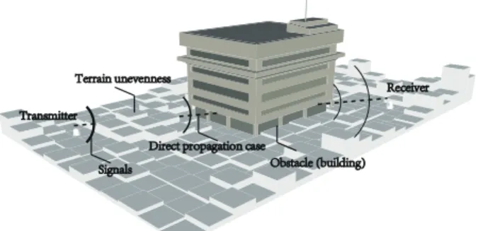
1) Path Loss: The wireless signal is dissipated along the propagation path; additionally, when encountering obstacles
Transmitter
Receiver
Signals
Direct propagation case
Obstacle (building) Terrain unevenness
Fig. 1: Illustration of obstacle processing.
(e.g., buildings), the signal is reflected, scattered, diffracted or absorbed [30]. PP L= 10nlog10d+ N X i=1 l(i)α(i)i−1 (3)
wherePP Lis the path loss of the signal power;n∈[2,5]is the path loss coefficient; dis the distance between the transmitter T X and the receiverRX;N is the number of obstacles (e.g. buildings) along the direct path from the transmitter and the receiver;l(i)is the exponent of attenuation of obstaclei; and α(i) is the penetration rate of obstacle i, which is within the range of [0,1], and α(i)i−1 indicates that the longer the distance between the transmitter and the obstacle, the less its effect to the signal intensity.
According to the works of [34], [35], we set the path loss exponent n as 3.0. In the equation 3, for a direct path, d is the distance betweenT X andRX, while for a reflected path, dis the distance between the virtual source and RX.
2) Graph-based 3D SPM: The proposed graph-based 3D SPM is derived from the work of [30]. In [30], the graph theory is utilized to detect edges and feature points, which were combined to identify obstacles. In this paper, the concept of LOS [29] used in [11] is employed and extended to simulate the direct and reflected wireless signals from the transmitter to the receiver and recognize obstacles along this signal.
As illustrated in Fig. 1, for rough urban terrain, the signal can be blocked by buildings or a rise in the ground, while if the terrain is flat, the only obstacle is the building.Specifically, the details are provided in Algorithm 1. First, we figure out the differences of the two points along the X and Y axes, respectively as in Line 2. Then, we check points along the axis with larger difference as in Line 3 or 30. In checking a point, if the other coordinate is also an integer, is coincides with a point in the terrain matrixmap, and the stored height is referred to, otherwise, two stored heights of adjacent points are considered and the higher one is cached as in Lines 10-17. And it will be compared with that of the point (Line 8) in the line connecting the two positions. If the line is in an obstacle, Lines 18-26 will be invoked. If the line is in free space previously (Line 20), an obstacle is occurred, and its type will be recorded and the counter will increase by 1. Additionally, if the line enters the building from the terrain, the type is updated to the building (Line 25). If the line is in free space, we update the tag (Line
Algorithm 1: LOS
Data: Positions of the transmitter and receiver:(i, j, h1)
and(a, b, h2)
Result: Number of obstacles:Nob, types of obstacles: Tob.
1 Nob= 0,T ag=−1; 2 ∆x=|a−i|,∆y=|b−j|; 3 if∆x≥∆y andi6=a then
/* Check points along the X axis */
4 Record the number of coordinates between the transmitter and receiver along theX axis asx1; 5 Record the slopes ask= (double)b−j
a−i and k1 = (double)h2−h1
a−i ; 6 form= 1 to∆x−1do
/* Compute the coordinate of the
next point */ 7 x2 =i+x1×m,y2 =j+k×(x2−i); 8 z=h1 +k1×(x2−i); 9 ify2 == (int)y2then 10 x3 = (int)x2,y3 = (int)y2; 11 z1 =map[x3] [y3]; 12 else 13 x3 = (int)x2,y3 = (int)y2; 14 z1 =map[x3] [y3]; 15 y3 =y3 + 1; 16 z2 =map[x3] [y3]; 17 z1 = max (z1, z2); 18 ifz < z1 then /* An obstacle occurs */ 19 ifT ag <1then 20 T ag= 1; 21 ifz1≥hmax then /* Building */ 22 Tob[Nob+ +] = 1; 23 else /* Terrain undulation */ 24 Tob[Nob+ +] = 0; 25 ifz1≥hmax then
/* From terrain to building */ 26 Tob[Nob−1] = 1; 27 else /* Free space */ 28 ifT ag== 1then 29 T ag= 0; 30 if∆x <∆y andj 6=b then
/* The similar procedure is invoked
27). Finally, we will obtain the number of obstacles and the corresponding types (Line 1).
For the reflection case, the graph theory is employed to trace the reflected line fromT XtoRX. Simultaneously considering the direct and reflected signal cases, the final path loss ofT X toRXcan be calculated following the procedure of Algorithm 2.
And the fitness function is as follows:
fCQ= 1 2 PNS′ i=1 PNSR,inb j=1 P P L SR,i,j PNS′ i=1N nb SR,iPth,SRP L + PNR′ i=1 PNRR,inb j=1 P P L RR,i,j PNR′ i=1N nb RR,iPth,RRP L (4) wherefCQ is the fitness value of the objectiveConnectivity
Quality; PP L
SR,i,j (PRR,i,jP L ) denotes the path loss value of sensor i(relay node i) and its neighbor relay nodej; PP L
th,SR (PP L
th,RR) denotes the path loss threshold of sensor node (relay node);N′
S (NR′) is the number of feasible sensor nodes (relay nodes) deployed outside obstacles; and NSR,inb (NRR,inb ) is the number of neighboring relay nodes that can communicate with sensor i (relay node i) through wireless signals, that is, the corresponding path loss is belowPth,SRP L (Pth,RRP L ).
C. Lifetime
In the considered network, there are two types of nodes: sensor nodes and relay nodes. The former is responsible for the monitor of the environment and information transmission to the latter; while the latter is in charge of collecting information from sensor nodes or other relay nodes, and transmitting data to another relay node or the sink node. Correspondingly, each sensor node selects the relay node with least path loss to join its cluster. As a result, each relay node will manage a bunch of sensor nodes, and its communication burden will be much more than a sensor node. Therefore, we focus on the lifetime of relay nodes, and the objective function is as follows:
fLT = max1≤i≤NR N RS i PRR,iP L NSPth,RRP L (5) where fLT denotes the fitness of the Lifetime objective; NR (NS) denotes the number of relay nodes (sensor nodes);NiRS denotes the number of sensor nodes, including the sensor in its cluster as well as those from other clusters when acting as a relay node for other relay nodes, the relay node iin charge of, here, if we see a relay node with less path loss to the sink node is nearer to the sink node, then, each relay node selects a nearest relay node nearer to the sink node as its next hop, otherwise, the sink is the destination; PRR,iP L denotes the path loss value between relay node iand its next hop.
D. Connectivity and Reliability Constraints
For the Connectivity constraint, each sensor node should be able to communicate with its cluster head (i.e., selected relay node), otherwise, a penalty value is added. For the relay nodes, assuming each relay as a vertex and the communication status of each two relay nodes as an edge, as a result, the
Algorithm 2: Path Loss of Propagation Signals
1 Initially, the reflection faces (i.e., building surfaces) are
recorded in advance;
2 For a T X, the reflection faces around it are put into a
queue;
3 InitializeP Lmin by the path loss of the direct signal; 4 whileThe queue is not emptydo
5 Pop up a reflection face from the queue;
6 Find out the intersection pointpsecof the virtual line
connecting the virtualT X and theRX;
/* The prior reflection face */
7 LetIparent denote the index of the prior reflection
face;
/* Initialize freespace tag */
8 Tf ree= 1;
/* Check out whether the signal is blocked before the last
reflection */
9 whilepsec is within the reflection faceand Tf ree and
Iparent≥0 do
10 Select elementIparent in the queue as the current
reflection face;
11 psec becomes the virtualRX;
12 The virtual T X is updated with respect to the
current reflection face;
13 Find out the new intersection pointpsec; 14 ifThe signal frompsec to the virtualRX is
blocked then
15 Tf ree= 0;
16 else
17 Tf ree= 1;
18 UpdateIparent;
19 ifpsecis within the reflection face andTf ree then /* The current last reflection
face */
20 LetP Ltmp denote the direct path loss from the
virtualT X and theRX, in which only obstacles within the currentpsec and theRX are
considered;
21 ifP Ltmp< P Lmin then 22 P Lmin=P Ltmp;
23 ifThe maximum volume of the queue is not reached
andthe reflection time of the current face is below the maximum valuethen
24 Push reflection faces around the current last
reflection face into the queue;
network can be represented as a graph. In this graph, one or more subcomponents are formed, within each of them, nodes can communicate with each other, while between any two nodes in different components, no communication path can be constructed. To find the subcomponents, we can traverse the graph, for which, many classic algorithms can be referred to.If the largest component size is less than the number of deployed relay nodes, that is to say, more than one subcomponents are formed, a penalty value is exerted.Specifically, we have:
pC= (NS−nS)×vp (6)
wherepCrepresents theConnectivityconstraint penalty value, nS denotes the size of the largest subcomponent, andvp is the penalty coefficient.
Because of energy depletion or accidents, in the deployed HWDSN, some node may collapse in advance, if it is a critical juncture in the connected route of two relay nodes, the connectivity of the whole network can be destroyed, and for the worst case, many nodes will be disconnected, therefore, reliability should be taken into consideration. To guarantee the reliability of the network, each sensor or relay node should be able to communicate with more than one relay node, otherwise, we add a penalty value. Mathematically, we have:
pR= NS X i=1 nSR,i+ NR X i=1 nRR,i ! ×vp (7)
nSR,i= max 0, Nth,R−NSR,inb
(8) nRR,i= max 0, Nth,R−NRR,inb
(9) where pR represents the penalty value of the Reliability
constraint,nSR,i(nRR,i) denotes the extra number of commu-nicable relay nodes of sensor node (relay node) i, andNth,R is the least number of relay nodes that each sensor node or relay node can communicate with.
E. Objective Summary
In the deployment optimization problem considered in this paper, HWDSNs and 3D urban terrain are considered. HWD-SNs are made up of heterogeneous directional sensors that have various sensing abilities as well as relay nodes. In the 3D urban terrain, there are buildings, and the ground can be even or rough.
There are three objectives: Coverage,Connectivity Quality and Lifetime as well as two constraints: Connectivity and Reliability being simultaneously considered. The objective Coverage is to maximize the coverage degree of the urban terrain. Thus, for a limited number of sensors, they should be scattered on the whole terrain as uniformly as possible. Nevertheless, for the objective Connectivity Quality, the aim is to minimize the path loss. For extreme situations, all sensor and relay nodes should be deployed in a very limited area, near the sink node. As to Lifetime, we mainly consider the relay node issue. By simultaneously considering these three objec-tives, the deployment quality can be more comprehensively guaranteed.
The fitness values are normalized to within the range of [0,1], and the aim of MOEAs is to simultaneously minimize them. For the penalty value, it should be larger than the maximum fitness value, in this paper, we simply set the coefficient asvp= 106
. The overall objectives are as follows:
min fCV +pC+pR fCQ+pC+pR fLT +pC+pR (10)
As the penalty value is several magnitudes larger than the maximum fitness values of all objectives, there exist numerous Pareto fronts, each of which corresponds to a penalty output. In other words, the penalty significantly affects the convergence of the solution set. And before the penalty value of 0 is achieved, the algorithm will focus on the convergence of the solutions.
F. Individual Representation
For the3-objective deployment problem, we employ several MOEAs for optimization, and novel MOEAs are also pro-posed. In an MOEA, a population comprised of a number of individuals is in evolution. Each individual is a candidate solution for the deployment problem, in which a gene de-notes a sensor (relay) node. Each sensor node is represent-ed by its position and sensing direction, while each relay node is encoded by its position. For example, an individual is in the following form: sS1, . . . , sSNS, sR1, . . . , sRNR
and sS i = xSi, yiS, θih, θvi , i = 1, . . . , NS, sR j = xRj, yjR , j = 1, . . . , NR; here, sSi represents sensor i, which is denoted by its deployment position xS
i, yiS
on the terrain and its horizontal sensing directionθh
i and vertical sensing direction θv
i, while sRj represents relay node j, denoted by its position xR
j, yjR
.
III. PROPOSEDALGORITHMS
To address the proposed 3-objective deployment opti-mization problem, we put forward novel distributed par-allel MOEAs, which are based upon the message pass-ing interface (MPI)-based distributed parallel cooperative co-evolutionary multiobjective co-evolutionary algorithm (DPCC-MOEA) [36], namely, DPCCMOEA with multiple populations (DPCCMOEA-MP).
A. Overview
Same to DPCCMOEA, DPCCMOEA-MP is based on the framework of Multiobjective Evolutionary Algorithm Based on Decomposition (MOEA/D) [37]. That is to say, in the popu-lation, each individual solves the problem of the weighted sum of all objectives; each individual corresponds to a different weight vector, and all individuals cooperate with each other to tackle the target multi-objective deployment problem. The procedure of DPCCMOEA-MP is illustrated in Algorithm 3.
Algorithm 3: DPCCMOEA-MP
1 Initialize parameters and allocate memory; 2 Group variables as detailed in Section III-C;
3 Calculate population importance values as in Section
III-B, and construct the parallel structure as in Section III-E;
4 Each CPU confirms the group of variables to evolve, as
well as identifies its population index and receives some individuals of the population as in Section III-E;
/* Main loop */
5 whileThe maximum generation number is not reacheddo 6 Exchange information among CPUs as in Section
III-F;
7 Each CPU selects a number of individuals as parents
to evolve the variables in the group as in Sections III-D1 and III-D2;
8 Crossover is performed to generate the remaining
variables of each offspring as in Section III-D3;
9 if Threshold is reachedthen
10 Update importance values and the parallel
structure as in Sections III-B and III-E;
11 Update threshold;
12 Refine all population to one population; 13 return The final population;
B. Population Adding
In DPCCMOEA, only one population is utilized, while in DPCCMOEA-MP, besides the main population optimizing all objectives,M subpopulations are also utilized, each of which optimizes one objective, here M is the number of objectives. During the evolutionary process, different attentions are paid to different populations, resulting in different variants of DPCCMOEA-MP, as follows:
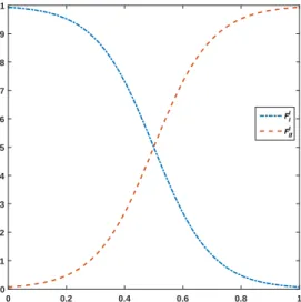
1) DPCCMOEA-MP-I: in the prophase, various popula-tions have nearly equal importances; while during the anaphase, more computation resources are consumed by the main population, as follows:
FII = 1.0
1.0 +e−10×(IT ERmaxIT ERmax−IT ERcur−0.5)
(11) where, IT ERcur denotes the current iteration number, andIT ERmaxrepresents the maximum iteration number. 2) DPCCMOEA-MP-II: the situation is opposite to that of
DPCCMOEA-MP-I, as follows: FIII =
1.0
1.0 +e−10×(IT ERmaxIT ERcur−0.5)
(12) 3) DPCCMOEA-MP-III: during the whole evolution
pro-cess, various populations have equal importance. For clarity, the changing behaviors ofFII andFIII are shown in Fig. 2.
C. Variable Grouping
On the 3D urban terrain, the sensor nodes to be deployed can be enormous, thus, according to section II-F, the number
Evolutionary Process 0 0.2 0.4 0.6 0.8 1 Importance Factor 0 0.1 0.2 0.3 0.4 0.5 0.6 0.7 0.8 0.9 1 FI I FI II
Fig. 2: Illustration of importance factor.
of variables in each individual can be large, resulting in a high-dimensional deployment optimization problem. To effectively tackle this kind of problem, separating variables to several groups and optimizing them under the cooperative coevolu-tionary (CC) framework [38] is a good choice. Naturally, the variables can be allocated to three groups: the positions of sensors, the sensing angles of sensors and the positions of relay nodes. In each group, variables are of the same property, facilitating the improvement of the optimization.
D. Evolution
1) Evolution of Subpopulations: As the subpopulations focus on optimizing their target objectives, in evolution, the best individual of the corresponding objective, updated after each generation, is referred to and the optimization strategy of DE/current-to-best/1 is employed. Here, we modify the parameter F in differential evolution (DE) [39]: according to the weight vectors, the larger the distance between the target individual and the best individual, the smaller the F. Additionally, the best individual in DE/current-to-best/1 is selected through tour selection to avoid being trapped in local optima.
2) Evolution of the Main Population: As to the main population, the evolution of individuals is the same as in DPCCMOEA.
3) Integration: After the evolution of a group of variables, in DPCCMOEA, this offspring is integrated with its parent and other two individuals. However, equal importance is put to its parent and other ones. To balance the exploration and exploitation abilities of the populations, with the processing of evolution, the possibility of integrating variables of the parent are increasing.
E. Parallel Structure
As multiple populations are utilized in DPCCMOEA-MP variants, a three-layer structure is constructed, which is based on a three-fold decomposition:
1) The 3-objective deployment optimization problem is de-composed and optimized by4populations: a main popu-lation for all objectives, as well as one subpopupopu-lation for each objective.
2) The variables are decomposed to several groups. Thus, each population is divided into severalsmall populations, each of which is responsible for a group of variables. 3) Individuals in each small population are allocated to a
number of sets; the purpose is that, more computation resources can be utilized and the algorithm can be adap-tive to different amount of resources.
Then, we can allocate the computation resources as follows: 1) The number of CPUs allocated to different populations
is proportional to the importance values.
2) The CPUs in the charge of each population are further uniformly allocated according to the number of small populationsin the corresponding population.
3) If one small population owns more than one CPU, the individuals in the small population are decomposed to several sets of equal size, each of which corresponds to one CPU.
During each step of evolution, in each CPU, the same number of individuals will be evolved, thus, for populations with less importance (less CPUs), less offsprings are produced. F. Communication
At the level of CPU, the von Neumann topology is formed [36]. In which, each CPU has four neighbors: the upper one, the lower one, the left one and the right one. Before each information transmission, one of the four directions is selected, and all CPU constructs the same data flow using the MPI parallel programming. The data for transmission can be the stored individuals, which can serve as reference information
during evolution. In usual, compared to computation, the communication among CPUs in distributed environment will be much time-consuming. While information sharing among CPUs contributes to the performance improvement. For the deployment problem considered in this paper, the objective functions are very time-consuming, so information can be exchanged more frequently.
IV. EXPERIMENTAL STUDY
A. Urban Terrains
There are two kinds of 3D urban terrains, even terrain and rough terrain, used in this paper; they are shown in Fig. 3, detailed as follows:
1) Terrain I (even): Fig. 3a, is derived from a region in a campus. The terrain is flat, the altitude of which is uniform, and there are several college buildings on the terrain. The size is185m×270m.
2) Terrain II (rough): Fig. 3b, is an artificial residential
quarter. The altitude difference of the ground is as high as 15.1490m and the highest position of which is even higher than the buildings in other positions. The rough terrain is of the size200m×230m.
(a) 3D urban terrain I
(b) 3D urban terrain II
Fig. 3: Illustration of 3D urban terrains.
The sampling resolution is5m, so the even terrain and the rough terrain are represented by 2D matrices with sizes37×54 and40×46, respectively.
There are various 3D scene acquisition methodologies. In [40], UAV was used to assist the reconstruction procedure by taking pictures at specified positions. Point cloud-based [41] method is popular, while can be time-consuming. He et al. [30] proposed a graph theory based methodology, which first detected feature points and edges, and then formed the struc-tures of buildings. Therefore, its efficiency is outperforming and can be applied to large-scale reconstruction of smart city. B. Parameter Settings
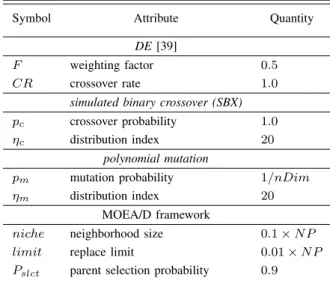
The proposed MOEAs are compared with Cooperative Co-evolutionary Generalized Differential Evolution 3 (CCGDE3) [42], Cooperative Multi-Objective Differential Evolution (C-MODE) [43], MOEA/D [37], Nondominated Sorting Genetic Algorithm III (NSGA-III) [44] as well as DPCCMOEA [36]. For the deployment optimization problem on each terrain, each algorithm runs 24 times. The number of fitness evaluations (FEs) for one run is set toD×103
, and D= 4NS+ 2NR is the number of variables, here, we setNS andNR to50 and 10, respectively.
For fair comparison, the population size of all algorithms is set toN P = 120. In CCGDE3, the fixed grouping is used, and the number of species is2, each of which has60individuals.
As there are3objectives, CMODE maintains3subpopulations with20individuals for each, and the archive size is120.The detailed parameter settings of algorithms are listed in Table I. For the proposed deployment problem, the path loss thresh-old of relay nodes is Pth,RRP L = 2 × Pth,SRP L . While for the remaining parameter settings, please refer to [11] and [45]. Additionally, in [11], σP AN and σT ILT vary in the range of [0.5,1.5], while in this paper, σP AN = 1 and σT ILT = 1.333333, as the screen aspect ratio is assumed to be4 : 3.
TABLE I: Algorithm Parameter Settings Symbol Attribute Quantity
DE[39]
F weighting factor 0.5
CR crossover rate 1.0 simulated binary crossover (SBX) pc crossover probability 1.0
ηc distribution index 20
polynomial mutation
pm mutation probability 1/nDim
ηm distribution index 20 MOEA/D framework
niche neighborhood size 0.1×N P
limit replace limit 0.01×N P
Pslct parent selection probability 0.9
C. Performance Indicator
For the 3-objective deployment optimization problem, we cannot solve it exactly through mathematical methods to obtain the optimal Pareto front (PF). Thus, indicators such as inverted generational distance (IGD), generational distance (GD), etc. [46] are unapplicable, instead, we use the hypervolume (HV) indicator [46], and the reference point is set as(1.0,1.0,1.0). Also, the final PF visualizations of all algorithms after the24 runs are provided.
D. Optimization Performance
For terrain I, Fig. 4a shows the evolutionary curves of averaged HV values of all runs generated by various al-gorithms; specifically, DPCCMOEA-MP-I reaches 0.7193, DPCCMOEA-MP-III reaches 0.7011, DPCCMOEA reaches 0.6175, NSGA-III reaches0.5985, DPCCMOEA-MP-II reach-es0.5946, CMODE reaches0.5733, MOEA/D reaches0.4210 and CCGDE3 reaches 0.3100.
DPCCMOEA and all DPCCMOEA-MP variants except DPCCMOEA-MP-II perform better than the counterparts. By comparing DPCCMOEA and all DPCCMOEA-MP variants, we can know the usage of subpopulations contributes to the performance improvement. The best strategy ought to be that employed in DPCCMOEA-MP-I, in which, subpopulations are given more importance during the prophase compare to the anaphase. From the performances of DPCCMOEA and DPCCMOEA-MP-II, there ought to be a fitness waste in subpopulations of II. In DPCCMOEA-MP-I, the subpopulations are mainly used in the prophase, but it differs little from DPCCMOEA-MP-III, in which the main population and subpopulations have equal importance during the whole process. The visualization of the approximated PFs of all runs obtained by all algorithms can be found in the supplementary material.
As to terrain II, the detailed average HV values are as follows: NSGA-III reaches 0.3533, CMODE reaches0.3222, DPCCMOEA reaches 0.2965, DPCCMOEA-MP-I reaches
0 0.5 1 1.5 2 FEs 105 0 0.2 0.4 0.6 0.8 HV Value Terrain I CCGDE3 CMODE MOEA/D NSGA-III DPCCMOEA DPCCMOEA-MP-I DPCCMOEA-MP-II DPCCMOEA-MP-III (a) 0 0.5 1 1.5 2 FEs 105 0 0.1 0.2 0.3 0.4 HV Value Terrain II CCGDE3 CMODE MOEA/D NSGA-III DPCCMOEA DPCCMOEA-MP-I DPCCMOEA-MP-II DPCCMOEA-MP-III (b)
Fig. 4: Evolutionary curves of average HV values of24 runs on terrain I and II.
0.2809, MOEA/D reaches0.2766, DPCCMOEA-MP-II reach-es0.2680, DPCCMOEA-MP-III reaches0.2629and CCGDE3 reaches0.2486, which are plotted in Fig. 4b.
The characteristics of different algorithms can be summa-rized in the following:
1) NSGA-III outperforms all other algorithms with consid-erable improvement.
2) Though CMODE converges slowly, it ranks the second with respect to the final result.
3) DPCCMOEA outperforms the multi-population variants, indicating the subpopulations are not beneficial for terrain II.
4) MOEA/D also overmatchs two multi-population variants, thus, MOEA/D is simple but powerful for terrain II. 5) CCGDE3 is still the worst.
For the visualization of the approximated PFs, please refer to the supplementary material.
From the optimization performances of various algorithms, we can summarize that, for different terrains, the performance
varies greatly. The multi-population strategy exhibits its pri-ority on terrain I, while all of them are inferior on terrain II.
E. Operation Time
The average operation times of all algorithms for one run are listed in TABLE II. We can see that, as distributed parallelism is employed in DPCCMOEA and DPCCMOEA-MP variants, much less time is consumed compared to other serial algo-rithms. Specifically, the experimental platform is the Tianhe-2 supercomputer and 72 CPUs are utilized, which is close to the speedups by comparing DPCCMOEA with CCGDE3 (i.e. 58.0), MOEA/D (i.e. 53.4), MOEA/DVA (i.e. 53.1) and NSGA-III (i.e.57.4). Therefore, we can say DPCCMOEA-MP variants can solve the multiobjective deployment optimization problem more effectively and efficiently.
V. CONCLUSION
In this paper, we study the 3D smart city-based multiob-jective deployment of HWDSNs by simultaneously consider-ing Coverage, Connectivity Quality and Lifetime as well as guaranteeing constraints of Connectivity and Reliability, for which, two 3D urban terrains (i.e. a real-world campus and an artificial residentialquarter) are utilized. For the signal propa-gation, a graph-based 3D model is presented via combining the LOS concept. To tackle the multiobjective deployment problem, based on DPCCMOEA, by utilizing subpopulations, several DPCCMOEA-MP variants are proposed. By verifying DPCCMOEA, DPCCMOEA-MP variants and other state-of-the-art MOEAs on the two 3D urban terrains, we find that the proper usage of subpopulations contributes to the optimization performance improvement of DPCCMOEA. Additionally, the distributed parallelism greatly reduces the operation time. As a conclusion, the presented DPCCMOEA-MP algorithms can address the proposed multiobjective deployment problem more effectively and efficiently as to the optimization performance and operation time, respectively. For the future work, we will further improve DPCCMOEA-MP algorithms, specifically, as the difficulties of objectives are different, the importance values of subpopulations can be diverse and change during the evolution. Moreover,larger scale 3D urban terrain big data can be considered.For the reconstruction of 3D smart city, we will try to experiment other methodologies.Additionally, more objectives can be added and many-objective algorithms can be devised. In summary, as the proposed algorithms are parallel in nature, its efficiency is advantageous, thus, the proposed algorithms have wide applications in the future smart city.
REFERENCES
[1] B. Tang, Z. Chen, G. Hefferman, S. Pei, W. Tao, H. He, and Q. Yang, “Incorporating intelligence in fog computing for big data analysis in smart cities,”IEEE Transactions on Industrial Informatics, vol. 13, no. 5, pp. 2140–2150, Oct. 2017.
[2] O. M. Alia and A. Al-Ajouri, “Maximizing wireless sensor network coverage with minimum cost using harmony search algorithm,”IEEE Sensors Journal, vol. 17, DOI 10.1109/JSEN.2016.2633409, no. 3, pp. 882–896, Feb. 2017.
[3] Manju, S. Chand, and B. Kumar, “Maximising network lifetime for target coverage problem in wireless sensor networks,” IET Wireless Sensor Systems, vol. 6, DOI 10.1049/iet-wss.2015.0094, no. 6, pp. 192– 197, 2016.
[4] E. Tuba, M. Tuba, and D. Simian, “Wireless sensor network coverage problem using modified fireworks algorithm,” in 2016 International Wireless Communications and Mobile Computing Conference (IWCMC), Paphos, Cyprus, September 5-9, 2016, DOI 10.1109/IWCMC.2016.7577141, pp. 696–701, 2016. [Online]. Available: https://doi.org/10.1109/IWCMC.2016.7577141
[5] H. Ma and Y. Liu, On Coverage Problems of Directional Sensor Networks, pp. 721–731. Berlin, Heidelberg: Springer Berlin Heidelberg, 2005. [Online]. Available: https://doi.org/10.1007/11599463 70 [6] H. Teng, C. D. Wu, Y. Z. Zhang, and N. Hu, “Design of probabilistic
sensing model for directional sensor node,”Journal of Jiangnan Uni-versity (Natural Science Edition), vol. 11, no. 4, pp. 391–395, 2012. [7] T.-W. Sung and C.-S. Yang, “Voronoi-based coverage improvement
approach for wireless directional sensor networks,” Journal of Network and Computer Applications, vol. 39, DOI http://dx.doi.org/10.1016/j.jnca.2013.07.003, pp. 202 – 213, 2014. [Online]. Available: http://www.sciencedirect.com/science/article/pii/ S1084804513001501
[8] V. Akbarzadeh, C. Gagne, M. Parizeau, M. Argany, and M. A. Mostafavi, “Probabilistic sensing model for sensor placement optimization based on line-of-sight coverage,”IEEE Transactions on Instrumentation and Measurement, vol. 62, no. 2, pp. 293–303, Feb. 2013.
[9] S. Li, C. Xu, W. Pan, and Y. Pan, “Sensor deployment optimization for detecting maneuvering targets,” in International Conference on Information Fusion, pp. 1629–1635, 2005.
[10] T. Y. Lin, H. A. Santoso, K. R. Wu, and G. L. Wang, “Enhanced deployment algorithms for heterogeneous directional mobile sensors in a bounded monitoring area,”IEEE Transactions on Mobile Computing, vol. 16, DOI 10.1109/TMC.2016.2563435, no. 3, pp. 744–758, Mar. 2017.
[11] B. Cao, J. Zhao, Z. Lv, and X. Liu, “3D terrain multiobjective de-ployment optimization of heterogeneous directional sensor networks in security monitoring,” IEEE Transactions on Big Data, vol. PP, DOI 10.1109/TBDATA.2017.2685581, no. 99, pp. 1–10, 2018.
[12] J. Li and M. Chen, “Multiobjective topology optimization based on mapping matrix and NSGA-II for switched industrial inter-net of things,” IEEE Internet of Things Journal, vol. 3, DOI 10.1109/JIOT.2016.2577889, no. 6, pp. 1235–1245, Dec. 2016. [13] M. Wolf, High-performance embedded computing: applications in
cyber-physical systems and mobile computing, pp. 501–521, 2014. [14] H. A. Salam and B. M. Khan, “IWSN - standards, challenges and future,”
IEEE Potentials, vol. 35, DOI 10.1109/MPOT.2015.2422931, no. 2, pp. 9–16, Mar. 2016.
[15] L. Wang, X. Fu, J. Fang, H. Wang, and M. Fei, “Optimal node placement in industrial wireless sensor networks using adaptive mutation probability binary particle swarm optimization algorithm,” in 2011 Seventh International Conference on Natural Computation, vol. 4, DOI 10.1109/ICNC.2011.6022417, pp. 2199–2203, Jul. 2011.
[16] P. Kuila and P. K. Jana, “Energy efficient clustering and routing algorithms for wireless sensor networks: Particle swarm optimization approach,” Engineering Applications of Artificial Intelligence, vol. 33, DOI http://dx.doi.org/10.1016/j.engappai.2014.04.009, pp. 127 – 140, 2014. [Online]. Available: http://www.sciencedirect.com/science/article/ pii/S0952197614000852
[17] S. Halder and S. D. Bit, “Enhancement of wireless sensor network lifetime by deploying heterogeneous nodes,” Journal of Network and Computer Applications, vol. 38, DOI http://dx.doi.org/10.1016/j.jnca.2013.03.008, pp. 106 – 124, 2014. [Online]. Available: http://www.sciencedirect.com/science/article/pii/ S1084804513000957
[18] X. Chu and H. Sethu, “Cooperative topology control with adaptation for improved lifetime in wireless sensor networks,”Ad Hoc Networks, vol. 30, DOI http://dx.doi.org/10.1016/j.adhoc.2015.03.007, pp. 99 – 114, 2015. [Online]. Available: http://www.sciencedirect.com/science/ article/pii/S1570870515000578
[19] G. Hacioglu, V. F. A. Kand, and E. Sesli, “Multi objective clustering for wireless sensor networks,” Expert Syst. Appl., vol. 59, DOI 10.1016/j.eswa.2016.04.016, no. C, pp. 86–100, Oct. 2016. [Online]. Available: https://doi.org/10.1016/j.eswa.2016.04.016
[20] K. Deb, A. Pratap, S. Agarwal, and T. Meyarivan, “A fast and elitist multi-objective genetic algorithm: NSGA-II,”IEEE Trans. Evol. Com-put., vol. 6, no. 2, pp. 182–197, Apr. 2002.
TABLE II: Average Operation Times (secs) of CCGDE3, CMODE, MOEA/D, NSGA-III, DPCCMOEA, DPCCMOEA-MP-I, DPCCMOEA-MP-II and DPCCMOEA-MP-III for Each Terrain.
CCGDE3 CMODE MOEA/D NSGA-III DPCCMOEA DPCCMOEA-MP-I DPCCMOEA-MP-II DPCCMOEA-MP-III
I 1.35E+04 (5.99E+01) 1.38E+04 (6.11E+01) 1.24E+04 (5.52E+01) 1.30E+04 (5.79E+01) 2.25E+02 1.99E+02 2.18E+02 1.94E+02
II 1.24E+04 (6.22E+01) 1.28E+04 (6.41E+01) 1.22E+04 (6.12E+01) 1.23E+04 (6.18E+01) 1.99E+02 1.94E+02 2.03E+02 1.93E+02
SUM 2.59E+04 (6.10E+01) 2.65E+04 (6.25E+01) 2.46E+04 (5.80E+01) 2.53E+04 (5.97E+01) 4.24E+02 3.93E+02 4.21E+02 3.87E+02
1Values in parentheses denote the speedups with respect to those of DPCCMOEA. 2Values in bold indicate better results.
[21] J. Jia,Coverage control and node deployment technologies in wireless sensor networks. Shenyang: Northeastern University Press, 2013. [22] J. Kennedy and R. Eberhart, “Particle swarm optimization,” inNeural
Networks, 1995. Proceedings., IEEE International Conference on, vol. 4, DOI 10.1109/ICNN.1995.488968, pp. 1942–1948 vol.4, Nov. 1995. [23] F. M. Al-Turjman, H. S. Hassanein, and M. A. Ibnkahla, “Efficient
deployment of wireless sensor networks targeting environment monitoring applications,” Computer Communications, vol. 36, DOI https://doi.org/10.1016/j.comcom.2012.08.021, no. 2, pp. 135 – 148, 2013. [Online]. Available: http://www.sciencedirect.com/science/article/ pii/S0140366412003106
[24] F. M. Al-Turjman, H. S. Hassanein, and M. Ibnkahla, “Quantifying connectivity in wireless sensor networks with grid-based deployments,” Journal of Network and Computer Applications, vol. 36, DOI https://doi.org/10.1016/j.jnca.2012.05.006, no. 1, pp. 368 – 377, 2013. [Online]. Available: http://www.sciencedirect.com/science/article/ pii/S1084804512001361
[25] K. Alexandris, G. Sklivanitis, and A. Bletsas, “Reachback WSN connec-tivity: Non-coherent zero-feedback distributed beamforming or TDMA energy harvesting?”IEEE Transactions on Wireless Communications, vol. 13, DOI 10.1109/TWC.2014.2330295, no. 9, pp. 4923–4934, Sep. 2014.
[26] L. Shu, M. Mukherjee, D. Wang, W. Fang, and Y. Chen, “Poster ab-stract: Prolonging global connectivity in group-based industrial wireless sensor networks,” in2017 16th ACM/IEEE International Conference on Information Processing in Sensor Networks (IPSN), pp. 325–326, Apr. 2017.
[27] H. R. Topcuoglu, M. Ermis, and M. Sifyan, “Positioning and utilizing sensors on a 3-D terrain part I — theory and modeling,”IEEE Trans-actions on Systems, Man, and Cybernetics, Part C (Applications and Reviews), vol. 41, DOI 10.1109/TSMCC.2010.2055850, no. 3, pp. 376– 382, May. 2011.
[28] S. Temel, N. Unaldi, and O. Kaynak, “On deployment of wireless sensors on 3-D terrains to maximize sensing coverage by utilizing cat swarm optimization with wavelet transform,” IEEE Transactions on Systems, Man, and Cybernetics: Systems, vol. 44, DOI 10.1109/TSMC-C.2013.2258336, no. 1, pp. 111–120, Jan. 2014.
[29] D. Hearn and M. P. Baker,Computer Graphics. Englewood Cliffs, NJ, USA: Prentice Hall, 1994.
[30] D. He, G. Liang, J. Portilla, and T. Riesgo, “A novel method for radio propagation simulation based on automatic 3D environment reconstruc-tion,” in2012 6th European Conference on Antennas and Propagation (EUCAP), DOI 10.1109/EuCAP.2012.6206457, pp. 1445–1449, Mar. 2012.
[31] Z. Yun and M. F. Iskander, “Ray tracing for radio propagation modeling: Principles and applications,” IEEE Access, vol. 3, DOI 10.1109/AC-CESS.2015.2453991, pp. 1089–1100, 2015.
[32] R. Wang, W. G. Wan, and X. Z. Wang, “Non-additive collaborative information coverage for cellular-model deployment in sensor network-s,” inIET International Communication Conference on Wireless Mobile and Computing (CCWMC 2009), DOI 10.1049/cp.2009.1887, pp. 49–52, Dec. 2009.
[33] R. Wang, W. Cao, and W. Xie, “Fuzzy coverage for sensor networks,” Chinese Journal of Scientific Instrument, vol. 30, no. 5, pp. 954–959, May. 2009.
[34] K. Sohrabi, B. Manriquez, and G. J. Pottie, “Near ground wideband channel measurement in 800-1000 MHz,” in1999 IEEE 49th Vehicular Technology Conference, pp. 571–574, 1999.
[35] H. Karl and A. Willig,Protocols and Architectures for Wireless Sensor Networks. New York, NY, USA: Wiley-Interscience, 2007.
[36] B. Cao, J. Zhao, Z. Lv, and X. Liu, “A distributed parallel cooperative coevolutionary multiobjective evolutionary algorithm for large-scale optimization,”IEEE Transactions on Industrial Informatics, vol. 13, DOI 10.1109/TII.2017.2676000, no. 4, pp. 2030–2038, Aug. 2017.
[37] Q. Zhang and H. Li, “MOEA/D: A multiobjective evolutionary algorithm based on decomposition,” IEEE Trans. Evol. Comput., vol. 11, no. 6, pp. 712–731, Dec. 2007.
[38] M. A. Potter and K. A. D. Jong, “A cooperative coevolutionary approach to function optimization,” inProceedings of the International Conference on Evolutionary Computation. The Third Conference on Parallel Problem Solving from Nature: Parallel Problem Solving from Nature, ser. PPSN III, pp. 249–257. London, UK, UK: Springer-Verlag, 1994. [Online]. Available: http://dl.acm.org/citation. cfm?id=645822.670374
[39] R. Storn and K. Price, “Differential evolution – a simple and efficient heuristic for global optimization over continuous spaces,” Journal of Global Optimization, vol. 11, DOI 10.1023/A:1008202821328, no. 4, pp. 341–359, 1997. [Online]. Available: http://dx.doi.org/10.1023/A: 1008202821328
[40] X. Zheng, F. Wang, J. Xia, and X. Gong, “The methodology of uav route planning for efficient 3d reconstruction of building model,” in2017 25th International Conference on Geoinformatics, DOI 10.1109/GEOINFOR-MATICS.2017.8090905, pp. 1–4, Aug. 2017.
[41] S. Barone, A. Paoli, and A. V. Razionale, “Three-dimensional point cloud alignment detecting fiducial markers by structured light stereo imaging,” Machine Vision and Applications, vol. 23, DOI 10.1007/s00138-011-0340-1, no. 2, pp. 217–229, Mar. 2012. [Online]. Available: https://doi.org/10.1007/s00138-011-0340-1
[42] L. M. Antonio and C. A. C. Coello, “Use of cooperative coevolution for solving large-scale multi-objective optimization problems,” in2013 IEEE Congr. Evol. Comput., pp. 2758–2765, Cancun, Mexico, 2013. [43] J. Wang, W. Zhang, and J. Zhang, “Cooperative differential evolution
with multiple populations for multiobjective optimization,”IEEE Trans-actions on Cybernetics, vol. 46, DOI 10.1109/TCYB.2015.2490669, no. 12, pp. 2848–2861, Dec. 2016.
[44] K. Deb and H. Jain, “An evolutionary many-objective optimization algorithm using reference-point-based nondominated sorting approach, part I: Solving problems with box constraints,”IEEE Transactions on Evolutionary Computation, vol. 18, DOI 10.1109/TEVC.2013.2281535, no. 4, pp. 577–601, Aug. 2014.
[45] D. He, J. Portilla, and T. Riesgo, “A 3D multi-objective optimization planning algorithm for wireless sensor networks,” in IECON 2013 -39th Annual Conference of the IEEE Industrial Electronics Society, DOI 10.1109/IECON.2013.6700019, pp. 5428–5433, Nov. 2013.
[46] E. Zitzler, L. Thiele, M. Laumanns, C. M. Fonseca, and V. G. da Fonse-ca, “Performance assessment of multiobjective optimizers: An analysis and review,” IEEE Trans. Evol. Comput., vol. 7, no. 2, pp. 117–132, Apr. 2003.
View publication stats View publication stats