Trade Costs and the Home Market Effect

Matthieu Crozet

Federico Trionfetti

No 2007

-February

Contents

1. INTRODUCTION 10

2. RELATIONSHIP TO THE LITERATURE 11

3. THE MODEL 12

3.1. Finite Elasticities (1< σA=σM <∞). . . 14 3.2. Perfect substitutability in the CRS-PC good (σA=∞). . . 17 3.3. Theoretical conclusion. . . 18 4. EMPIRICAL IMPLEMENTATION. 18 4.1. Data . . . 19 4.2. Estimations . . . 20 5. CONCLUSION. 26 6. APPENDIX 28

6.1. Finite Elasticities: results from numerical methods . . . 28

6.2. Perfect substitutability in the CRS-PC good: analytical results . . . 30

TRADECOSTS AND THEHOMEMARKETEFFECT

SUMMARY

Models characterized by the presence of increasing returns, monopolistic competition, and trade costs typically give rise to a more-than-proportional relationship between a country’s share of world production of a good and its share of world demand for the same good. This relation between country’s market size and industrial spe-cialization has become known as the Home Market Effect after Krugman (1980) and Helpmand and Krugman (1985). The HME is so closely associated to the presence of increasing returns to scale (IRS) and monopolistic competition (MC) that it has been used as a discriminating criterion in a novel approach to testing trade theory pioneered by Davis and Weinstein (1999, 2003).

However, Davis (1998) shed doubt on the theoretical robustness of this relationship. Indeed, one pervasive assumption in the literature to date is that of the presence of an “outside good”, freely traded and produced under constant returns to scale (CRS) and perfect competition (PC) ; Davis (1998) shows that in the absence of an outside good (i.e. assuming trade costs in all sectors), the HMEmaydisappear. The assumption of the existence of a freely traded CRS-PC good is as much convenient as it is at odds with reality. As noted by Head and Mayer (2004, p. 2634) when discussing this issue in their comprehensive account of the literature:“... the CRS sector probably does not have zero trade costs or the ability to absorb all trade imbalances.” The pervasive use of the outside good assumption and its inconsistency with reality raise the question of what are the consequences of its removal on the HME. The present paper investigates this question.

We eliminate the outside good from the main model used in the empirical literature on the HME. This model, in two different variants, has been used in Davis and Weinstein (1999, 2003) and in Head and Ries (2001). We find that, in general, the HME survives when the outside good is absent but its average magnitude is attenuated. More interestingly, both variants of the model predict a non-linear relationship between the production share and the demand share. The non-linearity is characterized by a weak HME (or absence thereof) when countries’ demand shares are not too different from the world average. The HME becomes stronger when countries’ demand share become more dissimilar.

In order to put this result to empirical verification, we use the trade and production database developed by CEPII (see Mayer and Zignago, 2005). Because of numerous missing values, we finally use a restricted balanced data set for 25 countries and 25 industries, over the period 1990-1996. Nevertheless, the set of countries remains very large; in 1996, it accounted for more than 78% of world GDP and about 70% of world trade.

In a fist step we estimate a polynomial equation relating countries’ relative demand for each good (i.e. the demand deviation from the sample average), to the corresponding production deviation. Demand deviations are computed as the sum of sectoral expenditures in all locations weighted by accessibility to consumers. We use Head and Ries (2001)’s measure of trade freeness to weight countries demand. The results strongly support the theoretical predictions: we observe a significant Home Market Effect on average, and a smoothly non-linear relationship between demand deviations and production deviations. We perform also several robustness checks. For instance, we follow Davis and Weinstein (2003) using a two step procedure to estimate the freeness of trade. First, we perform, for each industry, a gravity estimation using bilateral trade data; then the coefficients of this regression are used to compute the bilateral trade barrier. The results remain barely unchanged: the HME is smaller when absolute value of demand deviations from the average are small.

In a second step, we go further by estimating the critical value of demand deviations beyond which the HME has a stronger influence on specializations. We thus perform with maximum-Wald tests for each industry. We show that the relation between demand and production deviations is strictly linear for two industries only: Wearing apparel and rubber products.

One industry (Footwear) shows a non-linear shape that is clearly consistent with the constant-return to scale and perfect competition paradigm. Finally, for eleven industries (out of 25), we observe a “piecewise” HME: the relationship between output and demand deviations is proportional for medium-sized demand deviations, and more than proportional for very large and very low demand deviations. For these eleven industries (that account all together for more than 62% manufacturing production in our sample) the HME matters only for one fifth of the observations, and HME is of negligible importance or totally absent for the remaining observations.

ABSTRACT

Most of the theoretical and empirical studies on the Home Market Effect (HME) assume the existence of an “outside good” that absorbs all trade imbalances and equalizes wages. We study the consequences on the HME of removing this assumption. The HME is attenuated and, more interestingly, it becomes linear. The non-linearity implies that the HME is more important for very large and very small countries than for medium size countries. The empirical investigation conducted on a database comprising 25 industries, 25 countries, and 7 years confirms the presence of the HME and of its non-linear shape.

JELclassification: F1, R12.

COÛTS DE TRANSPORTS ET L’EFFET DU MARCHÉ DOMESTIQUE

RÉSUMÉ

Les modèles issus des nouvelles théories du commerce international, qui prennent en considération les rende-ments d’échelle croissants et les coûts de transport, montrent que les grands pays ont l’avantage de pouvoir s’appuyer sur leur vaste marché intérieur pour développer des spécialisations dans les secteurs à rendements croissants. En d’autres termes, il existerait une relation plus que proportionnelle entre la production relative des pays et leur demande relative. Depuis Krugman (1980), cette relation entre l’importance du marché in-térieur et la spécialisation industrielle est appeléeHome Market Effect(effet du marché domestique). Cet effet du marché domestique est associé de façon tellement étroite à la présence des rendements croissants et à la concurrence monopolistique que Davis et Weinstein (1999, 2003) l’ont utilisé comme test discriminant des théories du commerce. Les secteurs qui font ressortir un effet du marché domestique sont en concurrence imparfaite et doivent être étudiés à l’aide des nouvelles théories du commerce ; pour les autres, les théories traditionnelles fondées sur les avantages comparatifs conservent toute leur pertinence.

Cependant, Davis (1998) a remis en question la robustesse théorique de cette relation. En effet, la plupart des modèles qui mettent en évidence un effet du marché domestique retiennent l’hypothèse d’un «bien ex-térieur», en concurrence parfaite, et dont l’échange ne supporte aucun coût de transport. Davis (1998) montre qu’en revenant sur cette hypothèse, c’est-à-dire en supposant qu’il existe des coûts de transport dans tous les secteurs manufacturés, l’effet du marché domestiquepeutdisparaître. Ce résultat théorique est important dans la mesure où l’hypothèse d’un bien échangeable sans coût de transport est aussi commode, d’un point de vue théorique, que contraire à la réalité la plus évidente.

Dans cet article, nous étudions en détail les conséquences sur l’effet du marché domestique de l’abandon de l’hypothèse de bien extérieur. Nous proposons deux variantes d’un modèle proche de ceux présentés par Davis (1998) et Head et Ries (2001). A chaque fois, nous supposons qu’il y a des coûts de transport dans tous les secteurs. On montre que dans les deux versions du modèle, l’effet du marché domestique résiste à l’abandon de l’hypothèse de bien extérieur. La relation entre la demande relative et la production relative est néanmoins atténuée, et elle devient surtout non-linéraire. En effet, l’effet du marché domestique est plus faible (voire simplement absent) quand la différence de taille entre les pays est relativement faible ; il devient plus fort au fur et à mesure que les différences de demande relative augmentent. En d’autres termes, notre modèle montre que la différence de taille des pays ne peut affecter significativement les spécialisations et les échanges commerciaux qu’à condition que ces différences soient suffisamment prononcées. Ce résultat vient donc limiter les craintes de voir l’ouverture commerciale favoriser les grands pays au détriment des petits.

Les conclusions du modèle sont testées empiriquement en utilisant la base de données TradeProd, dévelop-pée par le CEPII (voir Mayer et Zignago, 2005). Nous retenons les données pour 25 pays et 25 secteurs, sur la période 1990-1996. Cet échantillon de pays est représentait, en 1996, environ 78 % du PIB mondial et 70 % du commerce mondial.

Dans un premier temps, nous estimons une équation non-linéaire associant la demande relative de chaque pays (i.e. la déviation de la demande par rapport à la moyenne de l’échantillon), à la production relative correspondante. Les demandes relatives sont calculées comme la somme des dépenses sectorielles dans chaque pays du monde, pondérées par une mesure des entraves au commerce. Ces coûts pesant sur les échanges commerciaux sont mesurés par l’indicateur proposé par Head et Ries (2001). Les résultats économétriques confirment clairement la pertinence des conclusions théoriques : on observe un effet du marché domestique moyen sur l’ensemble de l’échantillon, mais surtout, nous mettons en évidence le fait que cette relation est non-linéraire. Ce résultat résiste aux tests de robustesse que nous avons conduits, et notamment au changement de définition de l’indicateur mesurant les entraves au commerce. En utilisant un indicateur issu de l’estimation

d’une équation de gravité (comme dans Davis et Weinstein, 2003), nous obtenons des résultats tout à fait comparables.

Dans un second temps, nous allons plus loin en cherchant, pour chaque secteur, des points de ruptures dans l’effet du marché domestique, c’est-à-dire que l’on estime la valeur critique des déviations de demande au delà desquelles leur influence sur les spécialisations devient significativement plus forte. Nous montrons que la relation entre les déviations de demande et les déviations de production est strictement linéaire pour seulement deux secteurs : les produits d’habillement et le caoutchouc. Seule l’industrie de la chaussure donne des résultats conformes aux secteurs à rendements constants. Enfin, pour onze secteurs (sur 25), nous observons un effet du marché domestique en «ligne brisée» : le rapport entre la production relative et la demande relative est simplement proportionnel pour des déviations moyennes, et plus que proportionnel pour des déviations très grandes et très faibles. Par ailleurs, pour ces onze secteurs (qui représentent au total plus de 62 % de la production dans notre échantillon), l’effet du marché domestique n’a aucune influence sur les spécialisations de la grande majorité des pays ; il n’affecte réellement qu’un cinquième des observations. Au total, nous confirmons que si l’effet du marché domestique contribue en effet à modeler la structure du commerce mondial, il n’a de influence véritablement observable que sur un nombre limité de pays et de secteurs.

RÉSUMÉ COURT

L’introduction de rendements d’échelle croissants dans les théories du commerce conduit à mettre en évidence une relation plus que proportionnelle entre la taille relative du marché intérieur et la spécialisation industrielle. C’est ce que Krugman (1980) appelle l’effet du marché domestique (en anglais,Home Market Effectou HME). C’est une relation importante dans la mesure où elle permet d’expliquer certains processus de structuration des échanges mondiaux, mais aussi la répartition des gains à l’échange et les effets d’agglomération spatiales des activités. Cependant, la plupart du temps, ce type de modèle suppose l’existence d’un «bien extérieur», en concurrence parfaite et librement échangeable. Dans cet article, nous étudions les conséquences de l’abandon de cette hypothèse bien peu réaliste sur l’effet du marché domestique. On montre que le HME est atténué, mais surtout qu’il devient non-linéaire. La non-linéarité implique que le HME compte davantage pour les pays très grands et très petits que pour des pays de taille moyenne. Une analyse empirique, conduite sur une base de données comportant 25 industries, 25 pays, et 7 années confirme les conclusions du modèle.

JELclassification : F1, R12.

T

RADE

C

OSTS AND THE

H

OME

M

ARKET

E

FFECT

Matthieu C

Federico T

1. INTRODUCTION

Models characterized by the presence of increasing returns, monopolistic competition, and trade costs typically give rise to what has become known as the Home Market Effect after Krugman (1980) and Helpmand and Krugman (1985). The Home Market Effect (HME) is defined as a more-than-proportional relationship between a country’s share of world production of a good and its share of world demand for the same good. Thus, a country whose share of world demand for a good is larger than average will have - ceteris paribus - a more than proportionally larger-than-average share of world production of that good.4 _{The HME is so closely associated}

to the presence of increasing returns to scale (IRS) and monopolistic competition (MC) that it has been used as a discriminating criterion in a novel approach to testing trade theory pioneered by Davis and Weinstein (1999, 2003). Since then, as it will be discussed below, further theoretical and empirical research has explored the robustness of the HME and has searched for additional discriminating criteria. One pervasive assumption in the literature to date is that of the presence of a good freely traded and produced under constant returns to scale (CRS) and perfect competition (PC). This good is often referred to as the “outside good”. The presence of the outside good serves two purposes. First, it guarantees factor price equalization, thereby improving grandly the mathematical tractability of models. Second, it offsets all trade imbalances in the IRS-MC good, thereby permitting international specialization. A different way of seeing the second point is that the outside good accommodates all changes in labor demand caused by the expansion or contraction of the IRS-MC sector, thereby allowing for the reaction of production to demand in the latter sector to be more than proportional. The assumption of the existence of a freely traded CRS-PC good is as much convenient as it is at odds with reality. As noted by Head and Mayer (2004, p. 2634) when discussing this issue in their comprehensive account of the literature:“... the CRS sector probably does not have zero trade costs or the ability to absorb all trade imbalances.” The pervasive use of the outside good assumption and its inconsistency with reality raise the question of what are the consequences of its removal on the HME. The present paper investigates this question.

We eliminate the outside good from the main model used in the empirical literature on the HME. This model, in two different variants, has been used in Davis and Weinstein (1999, 2003) and in Head and Ries (2001). We find that, in general, the HME survives when the outside good is absent but its average magnitude

1_{We are grateful to Thierry Mayer and Soledad Zignago for having provided us with data. We thank Tommaso Mancini} for helpful advices and Rosen Marinov for excellent research assistance. We are grateful to anonymous referees for their comments, which proved very useful in clarifying and improving the paper. Authors are grateful, respectively, to the ACI - Dynamiques de concentration des activités économiques dans l’espace mondialand to the Swiss National Funds for financial support.

2_{Université de Reims, CEPII & Centre d’économie de la Sorbonne (matthieu.crozet@cepii.fr).}

3_{GREQAM, Université de la Méditerranée; Graduate Institute of International Studies; and CEPII} (Fed-erico.Trionfetti@univmed.fr).

4_{An alternative definition of the HME often used in the literature is that a country whose share of demand for a good} is larger than average will be a net exporter of that good. In this paper we will always refer to the HME as the more than proportional relationship between the share of production and the share of demand.

is attenuated. More interestingly, both variants of the model predict a non-linear relationship between the production share and the demand share. The non-linearity is characterized by a weak HME (or absence thereof) when countries’ demand shares are not too different from the world average. The HME becomes stronger when countries’ demand share become more dissimilar. We put this result to empirical verification on a data set containing 25 countries, 25 industries and 7 years. The non-linearity predicted by both models is strongly present in the data. One interesting consequence of the non-linearity is that the HME is more important for countries whose magnitude of demand shares is very different from the average than for countries whose demand shares are closer to the average. Performing a test of structural change with unknown breakpoints shows indeed that the HME matters only for the largest and smallest demand share, accounting for about one fifth of the observations in the sample. For the remaining observations, the HME is of negligible importance or totally absent.

As for the CRS-PC sectors, the model shows that the less-than-proportional relationship between share of production and share of demand survives the absence of an outside good. This result, combined with the more than proportional relationship between share of production and share of demand in the IRS-MC industry, confirms the theoretical validity of the HME as a discriminating criterion to test trade theories even in the absence of an outside good. The empirical investigation in this paper finds little evidence of sectors exhibiting a less than proportional relationship.

The remainder of the paper is as follows. Section 2 discusses the related literature, section 3 presents the model and the theoretical results, section 4 presents the empirical results, and section 5 concludes. The appendix discusses the numerical method, derives further mathematical results, and describes the data in further detail.

2. RELATIONSHIP TO THE LITERATURE

In the model structures of Krugman (1980) and Helpman and Krugman (1985) the HME is a feature of the IRS-MC sectors and not of the CRS-PC sectors. Recent empirical research has used this discriminating criterion to test the empirical merits of competing trade theories. In their seminal contributions, Davis and Weinstein (1999, 2003) find stronger evidence of the HME at the regional level (Davis and Weinstein 1999) than at the international level (Davis and Weinstein 2003). Head and Ries (2001) consider a model where, in addition to the outside good and the IRS-MC good, there is also a CRS-PC good characterized by National Product Differentiation à la Armington (1969), henceforth referred to as CRS-PC-A. The CRS-PC-A good is produced under constant returns to scale and perfect competition but consumers perceive national product differently from foreign product. In such model, the IRS-MC good exhibits the HME while the CRS-PC-A good does not. Using data for U.S. and Canadian manufacturing they find evidence in support of both the IRS-MC and the CRS-PC-A market structure depending on wether within or between variations are considered.

Both Davis and Weinstein (1999 and 2003) and Head and Ries (2001) assume the existence of an outside good. Indeed, the very first investigation on the consequences of the absence of the outside good has been pioneered by Davis (1998). He eliminates the outside good from the model in Helpman and Krugman (1985) by introducing trade costs in the CRS-PC good. His theoretical paper has elegantly shown that in in the absence of an outside good the HMEmaydisappear. The HME disappears if and only if trade costs in the CRS-PC good are sufficiently high to impede international trade in this good. Does the HME survive and what shape does it take when trade costs in the CRS-PC good are not high enough to impede trade in this good? This question, which we address both theoretically and empirically in part of this paper, remains unanswered in Davis (1998). Other papers have addressed the issue of trade costs and international specialization without, however, fo-cusing on the shape of the HME or on the validity of the HME as discriminating criteria. In a theoretical paper, Amiti (1998) studies, among other things, how the pattern of specialization and trade varies with country size

when industries have different trade costs. Hanson and Xiang (2004) theoretically and empirically investigate the pattern of specialization and trade in a model where a continuum of IRS-MC goods differ in terms of elas-ticities of substitution and trade costs. Holmes and Stevens (2005) focus on how the pattern of trade varies across industries that differ in technology when there are equal trade costs in all sectors. While these papers address issues related to the one in the present study, their focus is different from ours.5 _{The robustness of the}

HME is the subject of investigation also in Head, Mayer and Ries (2002), yet with focus on the role of market structure rather than on the role of the outside good. They study the robustness of the HME to three different modeling assumptions concerning the market structure: Cournot oligopoly and homogenous good, monopo-listic competition with linear demand, and Cournot oligopoly with national product differentiation. They find that the first two types of market structure yield a linear relationship between the share of production and the share of demand. The third market structure, instead, give results that depend on the elasticity of substitution between domestic and foreign goods.6

3. THE MODEL

In this theoretical section we study the consequences that the absence of an outside good has on the HME. The model is characterized by the presence of two goods: a good produced under IRS-MC, namedM; and a good produced under CRS-PC, named A. The latter is differentiated by country of production à la Armington (1969). For notational convenience we shall refer to this good as the CRS-PC-A good. Individuals have the following two-tier utility function:U =Mγ_A1−γ_{, whereγ∈(0,1)is the expenditure share on good} M. Both goods are differentiated. GoodM is a CES aggregate of all varieties ofM produced in the world, M =³R_κ∈Ω(cM k)

σM−1

σM dk

´ σM σM−1

, whereΩis the set of of all the varieties ofM produced in the world,cM k is consumption of varietyk, andσM is the elasticity of substitution between any two varieties. GoodAis a CES aggregate of the domestic and foreign variety ofA,A=

³ (cA1) σA−1 σA _{+ (cA2)}σA −1 σA ´ σA σA−1 , wherecAiis consumption of countryi’s variety of goodAandσAis the elasticity of substitution between the domestic and the foreign variety ofA. GoodAis produced under constant returns to scale and perfect competition, there is an infinity of domestic producers and an infinity of foreign producers. Consumers perceive the domestically producedAas different from foreignAbut they perceive as identical the output of two producers in the same country. There is, therefore, product differentiation by country of production. That is, consumers care about the “made in” label. In models of trade in the spirit of Helpman and Krugman (1985) the CRS-PC good is assumed to be perfectly homogenous internationally; thus, domestic and foreignA are perfect substitute. Assuming perfect substitutability and absence of the outside good gives the knife-edge result that we derive in Section 3.2. However, we do not limit our investigation to the case of perfect substitutability. We allow for a more general case where the domestic and foreign CRS-PC goods are not perfect substitute. This slight generalization will allow us to verify the robustness of the knife-edge results generated by the assumption of perfect substitutability.

5_{Other papers have studied different manifestations of the HME while keeping the assumption of the existence of} an outside good whenever appropriate. Such papers include Weder (1995), Lundbäck and Torstensson (1999), Feenstra, Markusen and Rose (2001), Trionfetti (2001), Weder (2003), Yu (2005), and Brülhart and Trionfetti (2005).

6_{In the third market structure, for intermediate and high values of the elasticity of substitution there is no HME and the} relationship between production and demandmaybe non-linear. The model based on this market structure, however, is not suitable to address the question of the robustness of the HME to the absence of the outside good since it does not predict the HME for any value of parameters. Further, its structure makes it hardly comparable to the models most widely used for theoretical and empirical purposes.

>From utility maximization and aggregation over individuals in the same country we have the following demand functions: mii =p−_{M ii}σMP_{M i}σM−1γYi,mji =p−_{M ji}σMP_{M i}σM−1γYi,aii =p−_AiiσAP_AiσA−1(1−γ)Yi,aji = p−σA

Aji PAiσA−1(1−γ)Yi; wheremii indicates domestic residents’ demand for any of the domestic varieties of M,mjiindicates countryi’s imports of any of the varieties ofM,aiiindicates domestic residents’ demand for the domestic production ofA,ajiindicates countryi’s imports ofA(the first subscript indicates the country where the good is produced, the second subscript indicates the country where the good is sold). Demand functions depend on prices and income: pM iiandpM ij represent, respectively, the price in countryiandj of a variety produced ini;pAii andpAij represent, respectively, the price iniandj of goodAproduced in i;PM i = ³R κ∈Ωi(piik) 1−σM_{dk +} R κ∈Ωj(pjik) 1−σM_dk ´ 1 1−σM

is the CES price index ofM relevant for consumers in countryiandΩiis the set of varieties produced in countryi;PAi=

³ p1−σA

Aii + p1Aji−σA ´ 1

1−σA

is the CES price index ofArelevant for consumers ini; national income isYi =wiLi, wherewiandLiare, respectively, the wage and labor endowment in countryi.

We allow for iceberg transport costs in both sectors. Thus,τM ∈ (0,1]andτA ∈(0,1]represent forM andA, respectively, the the fraction of one unit of good sent that arrives at destination. It is convenient to compact notation by use the following definitions of freeness of trade: φM ≡ τMσM−1 ∈ (0,1], andφA ≡ τσA−1

A ∈(0,1]. Trade in anyone of these sector is freer when the correspondingphiis larger.

Production technology of any variety ofM exhibits increasing returns to scale. The labor requirement per qunits of output is:LM =F +aMq. The production technology ofAexhibits constant returns to scale. To save notation we assume that one unit of labor input produces one unit of output ofA. Profit maximization gives the following optimal prices:

pAii=wi, pM ii= σM σM−1aMwi, i= 1,2. (1) pAij= 1 τA pAii, pM ij= 1 τM pii, i6=j, i, j= 1,2. (2) The zero profit condition gives the firm’s optimal size, which turns out to be the same in both countries and for all firms:

qi = F

aM(σM −1), i= 1,2. (3)

Using demand functions and Walras’ law the equilibrium conditions in the goods market are:

pM11q1 = p 1−σM M11 γw1L1 p1−σM M11 n1+φMp1M−22σMn2 + φMp 1−σM M11 γw2L2 φMp1M−11σMn1+p1M−22σMn2 (4) pM22q2 = φMp 1−σM M22 γw1L1 p1−σM M11 n1+φMp1M−22σMn2 + p 1−σM M22 γw2L2 φMp1M−11σMn1+p1M−22σMn2 (5) pA11A1 = p 1−σA A11 (1−γ)w1L1 p1−σA A11 +φAp1A−22σA +φAp 1−σA A11 (1−γ)w2L2 φApA1−11σA+p1A−22σA (6)

L1 = A1+n1(F+aMq1) (7)

L2 = A2+n2(F+aMq2) (8)

The fifteen equations (1)-(8) determine the fifteen endogenous variables of the model. These are the eight prices: pA11,pA12j,pA22,pA21,pM11,pM12,pM22,pM21; firm’s optimal size in each country: q1,q2; the number of varieties ofM produced in each country:n1,n2; the production ofAin each country,A1,A2, and the relative wageω≡ w1

w2. The exogenous variables include all parameters and - importantly for our purposes - the size of countries, represented byL1 andL2, respectively. It is convenient at this point to make use of the following definitions of share variables: SN i ≡ _n1n₊i_n2, represents countryi’s share of world production ofM;SAi ≡ _A1A₊i_A2, represents countryi’s share of world production ofA; andSLi ≡ _L1L₊i_L2, represents countryi’s share of world endowment of labor. Given the assumption of identical preferencesSLi represents also country i’s share of world’s demand. Models in the vein of Helpman and Krugman (1985) predict a more than proportional relationship between a country’s share of production and its share of expenditure for IRS-MC sectors, this is the HME, that is: dSN i

dSLi >1. They also predict a less than proportional relationship

between the a country’s share of production and its share of expenditure for CRS-PC sectors, that is: dSAi

dSLi ∈

[0,1). These predictions obtain in the presence of an outside good. The contrast between the more-than-proportional relationship in IRS-MC sectors and the less than more-than-proportional relationship in the CRS-PC sectors constitutes a discriminating criterion usable for testing trade theories. We want to verify whether the HME and the discriminating criterion are robust to the absence of the outside good.

To verify the magnitude of the production-demand relationships we would have to solve the model for the endogenous variables from which we would compute the share variables and, from the explicit expressions for the share variables, we would obtain the derivatives dSN i

dSLi and

dSAi

dSLi. The system composed of equations (1)-(8)

does not yield algebraic solutions for the endogenous variables, except in the special case whereσA=∞. We therefore use comparative statics and numerical methods to obtain results for the case of a finite value ofσA. In the next two sections we study two cases which bring us close to two frameworks used in the literature related to our paper. In section 3.1 we will assume thatσA =σM. This assumption, abstracting from the absence of an outside good in our model, brings us to the framework used in Head and Ries (2001). In section 3.2 we will assume thatσA6=σM and thatσA =∞. The assumption corresponds exactly to the model in Davis (1998). In this special case, the model is solvable explicitly.

3.1. Finite Elasticities (

1

< σ

=

σ

<

∞).

Even when it is assumed that σA = σM ≡ σthe model remains algebraically unsolvable. We therefore obtain the results in two ways: first we perform a comparative statics exercise, second we explore the model numerically.

3.1.1. Comparative statics.

We differentiate the system composed of equations (1)-(8) at the symmetric equilibrium (SLi =1₂). We impart on the system an idiosyncratic shockdL1 =−dL2to the absolute size of countries. Given the assumption of identical preferences, the shock to the size of countries generates an idiosyncratic demand shock of the same magnitude. Total differentiation gives the derivatives of all the endogenous with respect todLi. Given that dSLi =_(L1dL₊i_L2)we can easily compute all the derivatives with respect todSLi, in particular we are interested in dni

dSLi and

dAi

derivatives of interest for our analysis, namelydSN i

dSLi and

dSAi

dSLi. The resulting expressions are long and intricate

and, therefore, not particularly informative. These expressions, however, simplify grandly if we compute them for equal trade costs in both sectors,φM =φA=φ. Thus, for expositional purposes, all expressions shown in this sub-section are computed at equal trade costs in both sectors. Naturally, in the numerical exploration of the model we relax this restriction. To make notation less tedious, henceforth we suppress the country subscripti since no possibility of confusion arises.

Total differentiation gives dSN dSL =

(1 +φ)2

(1−φ)2+ 4φγ >1, for anyφ∈(0,1]and anyγ∈[0,1). (9) The derivative in expression (9) is larger than one, therefore there is HME in the IRS-MC sector. Comput-ing the derivative for sectorAwe find:

dSA dSL

= (1−φ) 2

(1−φ)2+ 4φγ ∈[0,1), for anyφ∈(0,1]and anyγ∈[0,1). (10) The derivative in expression (10) is between zero and one, therefore there is a less than proportional reaction of production to demand in the CRS-PC-A sector.

The two derivatives above tell us that the discriminating criterion to test trade theories developed by Davis and Weinstein (1999, 2003) is robust to the absence of an outside good since we have found thatdSN/dSL>1 and thatdSA/dSL ∈[0,1). This notwithstanding, the absence of an outside good reduces the magnitude of the HME. To see this, we take the derivative ofdSN/dSL with respect toφA and (after differentiation) we evaluate it atφM =φA. This gives:

d ³ dSN dSL ´ dφA = 4 (1−γ) h (φ(1−φ)2) (σ−1) + 2γ¡1 +φ2¢_{σ−γ(1−φ)}2i (2σ−1 +φ) h (1−φ)2+ 4γφ i2 >0, (11)

The derivative is positive, which means that a decline of trade costs inA(i.e., an increase inφA) magnifies the HME inM. We can conclude that the absence of the outside good, although it does not eliminate the HME, reduces its intensity.

3.1.2. Numerical exploration of the model.

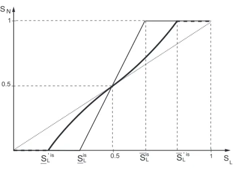
In the previous subsection we have found analytical results in a neighborhood of the symmetric equilibrium (SL = 1₂). In this section we want to find out the shape of the functional relationship between the share of production and the share of demand in the entire set of incomplete specialization. To this aim, we explore the model numerically. The numerical method is explained in section 6.1 of the appendix. Figure1illustrates the results obtained by use of numerical methods. The dotted line is the 45-degree line. The continuous straight line shows the functionSN(SL)within the incomplete specialization set in the presence of an outside good (like in Head and Ries, 2001). The incomplete specialization set is (Sis

L,SLis). Removing the outside good from the model makes the HME non-linear as shown by the thick line. This line represents the functionSN(SL) in the absence of an outside good in the new incomplete specialization set (S0is

L ,SL0is). The slope of the thick line is larger than one everywhere within the incomplete specialization set but it is flatter around the symmetric

equilibrium than away from it. This implies that the HME is weaker if country’s demand deviation from the world average are small than if they are large. We can conclude that the absence of the outside good makes the HME non linear. Further, it increases the size of the incomplete specialization set.

The functionSA(SL), not shown in the figure, is the mirror-image ofSN(SL)around the 45-degree line. That is,SA(SL)is convex forSL <1/2, it is concave forSL >1/2, and it has an inflection atSL = 1/2. Further, its slope is always less than one.

Figure 1: Smoothly non-linear HME

1 0.5 S_N 0.5 1 _S L

S

S

S

S

Figure1serves the purpose of illustrating the results but does not show an actual simulation. A striking feature of actual simulations is that the non-linearity ofSN(SL)is barely visible (see Figure4in the appendix). Although almost invisible, the non-linearity is present in all simulations (see appendix section 6.1).

The results from comparative statics and from numerical methods can be summarized in the following proposition.

Proposition 1. When elasticities are finite, the absence of the outside good does not eliminate the HME, it only reduces its magnitude and makes it non-linear; the non-linearity is tenuous, however.

To get the intuition for the non-linearity we start by noting that in a neighborhood of the symmetric equilib-rium (SL= 1/2) the HME is linear, indeed the functionSN(SL)has an inflection at the symmetric equilibrium (with slope larger than one). The initial increase ofSL, besides having an impact onSN, it also has a posi-tive impact on the relaposi-tive wage. Therefore, the effect of any subsequent increase ofSL on the demand for home goods is multiplied by a higher wage than any previous increase. Any subsequent increase ofSLwill be transmitted to the share of production through the familiar HME mechanism, though more strongly than any previous increase ofSL.

3.2. Perfect substitutability in the CRS-PC good (

σ

=

∞).

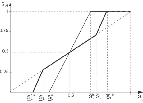
When good A is perfectly homogenous internationally (σA =∞) the resulting model is exactly as in Davis (1998). The major finding of Davis’ paper is that the HME disappears when trade costs inAare sufficiently high to eliminate trade in that good. Our focus is to study the shape of the HME when trade costs are not sufficiently high to eliminate trade inA. This aspect remains unexplored in Davis’s paper. We obtain explicitly all the results in section 6.2 of the appendix. Here, we summarize the results by use of Figure2.

As mentioned above, the HME disappears if trade costs are sufficiently high to impede trade inA. The intuition for this result is quite simple. IndustryM cannot expand more than proportionally because industry Acannot release labor. IndustryAcannot release labor because, if there is no trade inA, domestic production ofAmust satisfy domestic demand. In the absence of trade inA, a country’s share of production ofAmust be proportional to its share of demand. Consequently, the country’s share of production ofM must also be proportional to its share of demand. When trade inAoccurs then there is HME inM. The reason is that industryAno longer needs to satisfy domestic demand (goodAcan be imported) and therefore it can release labor to industryM, which can expand more than proportionally. The existence of the HME in this model, therefore, depends crucially on whether trade costs inAare high enough to eliminate trade in this good. The sufficient condition for the HME to exist isτA> τ

σM−1

σM

M (see appendix section 6.2).

Figure 2: Piecewise non-linear HME

1 0.75 0.5 0.25 0.5 1 S L S_N

S

S

S

S

S

S

Figure2summarizes the results. The continuous straight line represents the case of zero trade costs in A. This line represents the familiar form ofSN(SL)shown, for instance, in Helpman and Krugman (1985). The line shows that there is HME within the incomplete specialization set (SLisandSL

is

). The thick broken line represents the functionSN(SL)in the case of positive and not prohibitive trade costs inA. In this case the incomplete specialization set (S0

LisandSL0 is

that there is no HME within the set¡SL, SL ¢

but there is HME for values ofSLoutside this set and within the incomplete specialization set, where the relationship betweenSN andSL is more than proportional. An increase of trade costs inAwith respect to trade costs inM expands symmetrically the set¡SL, SL

¢ which then covers a larger section of the set(0,1)(the more-than-proportional sections of the broken line would shift away from the symmetric equilibrium). If trade costs inAare sufficiently high, then the set¡SL, SL

¢

coincides with(0,1)and the home market effect disappears completely.

The functionSA(SL), not shown in the figure, is the mirror-image ofSN(SL) around the 45-degree line. The relationship is less than proportional for SL < SL and for SL > SL; and it is proportional for SL∈(SL, SL). We can summarize the results as follows:

Proposition 2. WhenσA=∞, there is HME if the set

¡ SL, SL

¢

is a proper subset of(0,1).

When there is HME, the relationship between share of demand and share of production inMis represented by a broken line like the thick line in Figure2. We refer to this shape as the “piecewise HME”.

3.3. Theoretical conclusion.

The model examined in this section gives the following prediction: removing the outside good makes the HME non linear by either giving it the smooth shape (Figures1) or the piecewise shape (Figure2). The model gives also another prediction: the HME is weaker (if it exists at all) nearer the symmetric equilibrium than away from it. This means that the HME is more important for countries whose demand shares are very different from the world average than for countries whose demand shares are near the world average. In the empirical part we subject these results to empirical investigation.

4. EMPIRICAL IMPLEMENTATION.

The key result of the previous section is that the absence of an outside good attenuates the magnitude of the HME and makes it non linear. This non-linearity is a distinctive feature of the model and can be verified empirically by estimating the relationship between countries’ production shares and demand shares. Moreover, the empirical analysis of the shape of the HME allows us to identify the set of countries for which the HME is of negligible or null magnitude and those for which the HME is important.

Following Davis and Weinstein (2003) and Head and Ries (2001), we analyze, for a large set of countries and industries, the relation between each demand deviation from the sample average and the corresponding production deviation. Denoting withxiktthe quantity of goodk, produced in countryiat datet, production deviation in countryifor productkis:

SS,ikt= P_Rxikt i=1xikt

− 1 R,

whereRis the number of countries. SS,ikt is positive if the production of goodkin countryiis greater than the mean value of the sample, and negative otherwise. To be consistent with the theoretical model, we measureSS,iktin terms of quantity of production. We proxy the quantities byxikt =Xikt/pikt, whereXikt is the value of production of goodkin countryiat datetandpiktis the price of that production.

The demand deviation variable is defined similarly: SD,ikt= P_RDikt/pikt

i=1(Dikt/pikt)

− 1 R,

whereDiktis what Davis and Weinstein (2003) call the “Derived Demand” and Head and Mayer (2006) call the “Nominal Market Potential”. It is the value of demand emanating from all countries for good k produced in countryiat datet. It is computed as the sum of sectoral expenditures in all locations weighted by accessibility to consumers. Denoting withEjktthe expenditure on goodkin countryjand withΦijkta measure of trade freeness, we have:

Dikt= PR

j=1ΦijktEjkt.

An important issue for empirical investigation lies in the measurement of trade freeness represented by the parameterΦijkt. We use here the same estimate of trade barriers as Head and Ries (2001). Using the theoretical demands expressed on foreign and domestic markets and assuming symmetric bilateral trade freeness and free trade within countries, they obtain the following proxy forΦijkt:

ΦHRijkt= r

zijktzjikt ziiktzjjkt,

wherezijktis the value of the trade flow of goodk, fromitojat yeartandziiktis countryi’s imports from itself. The indexΦijktvaries from 0 (prohibitive trade barriers) to 1 (free trade).8

This measure of freeness of trade has three main qualities. Firstly,ΦHR

ijktis time-dependent, so that we can control for the potential changes in access to market due to trade liberalization processes. Secondly, ΦHR

ijktcatches all possible sources of bilateral trade barriers, besides trade frictions associated to geographical distances and other usual gravity inputs. Thirdly, ΦHR

ijkt does not impose any strict assumption on bilateral trade relation and fits specifically to each country-pair. For instance, the gravity equation assumes a log-linear influence of geographic distance on bilateral trade and cannot fit well for particularly large or small distances. This is very important for the purpose of this paper; since we are looking for nonlinearity in the HME relation, we have to make sure that our measure of access to market does not introduce a bias that especially affects outlier trading countries.

4.1. Data

The empirical investigation of the model requires compatible data of production and demand at the sectoral level. Moreover, we need bilateral trade data for the corresponding products and countries in order to compute ΦHR

ijkt.

We use the trade and production database developed by CEPII (see Mayer and Zignago, 2005).9 _{It uses}

CEPII’s database of bilateral trade (BACI10_{) and OECD-STAN to expand the trade and production database}

produced by the World Bank (the latter database comes from both COMTRADE and UNIDO).

CEPII’s database covers a large set of industrial sectors (ISIC-Rev. 2) and countries, over 25 years (1976-2001). It provides figures on sectoral production, prices, total exports and imports, and bilateral trade. For each country and sector, intra-national trade is computed as the difference between country’s sectoral production and its aggregate sectoral exports to all other nations. Similarly, domestic expenditure is the sum of this non-exported production and the sectoral imports from the rest of the world.

Because of numerous missing values, we finally use a restricted balanced data set for 25 countries and 25 industries, over the period 1990-1996 (Table8 in appendix gives a complete list of the countries and the industries in the database).11 _{Nevertheless, the set of countries remains very large; in 1996, it accounted for}

8_{Head and Mayer (2004) discuss further this index. See also Behrens et al. (2004).} 9_{The original database is available atwww.cepii.fr/anglaisgraph/bdd/TradeProd.htm.} 10_{http://www.cepii.fr/anglaisgraph/bdd/baci.htm}

11_{We tried to keep a large number of industries. We only dropped three of them from the original database (Furniture}

more than 78% of world GDP and about 70% of world trade.

Figure 3: Demand deviations and production deviations (1996)

0 .2 .4 0 .2 .4 -.2 -.2 45° line .6 .6 Ss =1.1 9x SD R²= 0.8 58 Fitte dlin e

Demand deviations

Production deviations

Figure3plotsSS,iktagainstSD,iktfor the 25 industries and the 25 countries. To get a more intelligible figure, we plot these only for the year 1996.12_{As expected, we observe that greater demand deviations increase}

production deviations more than proportionately (the fitted line has a slope of 1.19). We also observe that some observations with the largest positive demand deviations are above the fitted line, whereas the observations with the smallest demand deviations are mainly below the fitted line. This visual inspection confirms our theoretical prediction but it is by the use of econometric techniques that we will rigorously verify the presence of the non-linearity.

4.2. Estimations

By definition, the mean value of bothSS,iktandSD,ikt is zero. With such centered variables, the simplest estimable equation corresponding to the thick line drawn in Figure1is the following:

SS,ikt=α1SD,ikt+α2SD,ikt.|SD,ikt|, (12) The estimation of equation (12) gives all the information we need in order to infer the shape of the rela-tionship between share of production and share of demand. Indeed, it is easily verified that, if the estimated α2is positive, then negative demand deviations make the shape concave whereas positive demand deviations make the shape convex. Exactly the opposite applies ifα2is negative. Ifα2 = 0, then the HME is linear.13

12_{Of course, the choice of 1996 does not affect greatly what the figure looks like.} 13_{The estimated equation (12) has the following functional form:y=α1(x−}1

2)+α2(x− 1 2)|x−

1

2|.The first derivative

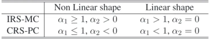
Thus, the estimated values of the coefficientsα1andα2 can be associated precisely with different shapes of the production-demand relationship and with different market structures as shown in Table1.14

Table 1: Coefficients, shape, and market structure

Non Linear shape

Linear shape

IRS-MC

α

≥

1

,

α

>

0

α

>

1

,

α

= 0

CRS-PC

α

≤

1

,

α

<

0

α

<

1

,

α

= 0

Econometric estimates of the model are presented in Tables2 to5. All regressions use ordinary least squares.

4.2.1. Pooled regressions: The basic result

We start by performing several pooled estimations of equation (12), i.e. for the 25*25*7=4375 observations. Results are in Table2.

Table 2: Pooled regressions

OLS estimates (1) (2) SD 1.189>1 1.146>1 (0.018) (0.021) SD.|SD| 0.261b (0.128) Nb. Obs. 4375 4375 R2 _{0.862 0.862}

Notes: SDis the computed derived demand deviation. Robust standard error in

paren-theses.a_,b_,c_{: Respectively significant at the 1%, 5% & 10% levels.}=1_,>1_:

Significant at the 1% level, and respectively equal and greater than one at the 5% level.

the estimated value ofα1is larger than1, the slope of the production-demand relationship is larger than1everywhere. The

second derivative is:y00_{=α2[2sign(x−}1

2) + (2x−1)Dirac(x− 1

2)]. Whenα2is positive, theny

00_Q0forxQ 1

2,

therefore the function is concave forx <1/2, it has an inflection atx= 1/2, and it is convex forx >1/2. The sign of

y00_{and the shape of the curvature are reversed when whenα}

2is negative. Ifα2 = 0the function is linear everywhere.

14_{One advantage of using (12) over a polynomial specification is that the latter gives rise to multicollinearity among the} odd-powered and the even-powered terms. On the contrary, multicollinearity diagnostics are systematically negative for equation (12).

Column (1) displays a benchmark estimation assuming a simple linear relation betweenSD,iktandSS,ikt. As expected, the coefficient is positive and greater than one, which indicates that there is, on average, a sig-nificant Home Market Effect. Moreover, the coefficient value of 1.189 is of comparable magnitude to those obtained by Head and Ries (2001) in the case of the between estimates. However, the main object of our interest is the estimated value ofα2in equation (12). This result is shown in column (2). The introduction of the second term reduces the estimated value ofα1, and the estimated value ofα2is unambiguously positive. These estimates indicate that the relation between demand shares and production shares is smoothly non-linear. Like in Figure 1, the Home Market Effect is always present, but its strength increases with the absolute size of demand deviations.

4.2.2. Pooled regressions: Robustness tests

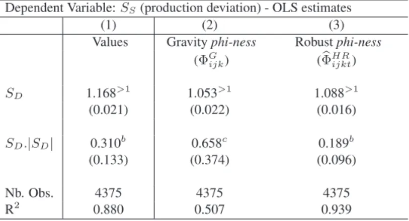
Tables3and4present a set of robustness checks of the result presented in Table2.

Table 3: Pooled regressions - Robustness tests

(1) (2) (3)

Values Gravityphi-ness Robustphi-ness (ΦG ijk) (ΦbHRijkt) SD 1.168>1 1.053>1 1.088>1 (0.021) (0.022) (0.016) SD.|SD| 0.310b 0.658c 0.189b (0.133) (0.374) (0.096) Nb. Obs. 4375 4375 4375 R2 _{0.880 0.507 0.939}

Notes: SD is the computed derived demand deviation. a,b,c: Respectively

significant at the 1%, 5% & 10% levels. =1_,>1_{: Significant at the 1%}

level, and respectively equal and greater than one at the 5% level. Robust standard errors in parentheses.

In Table3, we consider several alternative definitions of variables. First, column (1) reports the estimates of the model using values of production and demand rather than volumes. This specification is less relevant for the purpose of the present paper, but it allows us to compare the results with the previous literature. The results in column (1) of Table3are comparable to those shown in Table 2. Both coefficients are significantly positive andα1is greater than one, which reveals again a smoothly non-linear HME.

Another empirical issue that needs to be addressed concerns the measurement of trade impediments. As explained above,ΦHR

ijktis a measure of trade freeness that has many good features. However, as a robustness test, columns (2) and (3) of Table3display the results obtained using two alternative definitions ofΦijkt.

In column (2), we follow Davis and Weinstein (2003) using a two step procedure to estimate the freeness of trade. First, we perform, for each industry, a gravity estimation using bilateral trade data; then the coefficients of this regression are used to compute the bilateral trade barrier. Our specification follows Eaton and Kortum (2002) and Combes et al. (2005). We divide each international trade flow by the internal flow of the importer.

We denote withzijkt the exports of good kfrom country ito countryj,xikt the production of good kin countryi,piktthe price of that production,dijthe bilateral distance betweeniandjandCija dummy variable that equals one if countriesiandjhave a common border.εijktis an error term andt, as usual, denotes time. The gravity equation we estimate is:

ln µ zijkt zjjkt ¶ =b1ln µ xikt xjkt ¶ +b2ln µ pikt pjkt ¶ +b3ln µ dij djj ¶ +b4Cij+b5+εijkt.

This specification of the gravity equation allows to control for the importing country-specific price index that appears in structural bilateral trade equations. Here, the intercept (b5) is a measure of the border effect (b5 < 0). We estimate this equation separately for each industry. For all of them, the coefficients have the expected sign, therefore we can compute a time invariant gravity-based measure of trade freeness: ΦG

ijk = ³

db3k

ij ´ ¡

eb4kCij¢ ¡eb5kIntraij¢, whereIntra_ij is a dummy that takes the value one ifi=j.

We then useΦG

ijkto compute derived demand and estimate equation (12). The results shown in column (2) of Table3are consistent with those obtained usingΦHR

ijk; Bothα1andα2are positive andα1is significantly greater than one, which denotes a smoothly non-linear HME pattern. However, the overall fit of the model is relatively weak.

Finally, we consider the possibility thatΦHR

ijkt may be affected by measurement errors in bilateral trade flows and by sudden changes in prices of traded goods. Hence, we introduce a third measure of trade freeness,

b

ΦHR

ijkt, that is a robust measure ofΦHRijkt. We estimate the following equation:ln ΦHRijkt=²ij+²k+²t+νijkt, whereνijktis an error term and²ij,²k and²tare three sets of fixed effects, relative respectively to country pairs, industries and years. Hence,ΦHR

ijktis broken up into three elements. The first one (²ij) accounts for the influence of elements such as distances, bilateral trade agreements, common language, etc. The second one (²k) accounts for the differences in product transportability. The last one (²t) captures the evolution of transport techniques and multilateral trade agreements. We defineΦbHR

ijktas the exponential of the predicted value of this estimation. As expected,ΦbHR

ijkt is highly correlated toΦHRijkt, but its variance is smaller.15 The estimates of equation (12) usingΦbHR

ijktare reported in column (3). Once again, we confirm the results presented in Table2 that show a smoothly non-linear HME.

In Table4we test whether the result reported in Table2is robust to alternative specifications and country sampling. First we ran estimations using a data set restricted to OECD countries (see column 1).16 _When

non-OECD countries are excluded from the data,α2is non-significant, which gives support to the linear HME hypothesis. This is consistent with theory because intra-OECD demand deviations are less heterogeneous than they are in the full sample.

In column (2) we control for a possible bias resulting from temporary external imbalances by using the variableT Bikt. This variable is computed as the product of countryi’s trade balance and the share of i’s production of goodkin the world economy. Controlling for external imbalances does not change the results. Moreover, introducingT Biktyields a stronger smooth non-linearity;α1is smaller andα2is larger.

Finally, we estimate the model with different sets of fixed effects. As there is no intercept in the model, we always constrain the sum of the fixed effects to be equal to zero. In columns (3) and (4) we introduce respectively year and industry fixed effects. The results remain unchanged. In columns (5) and (6) we estimate

15_{Note that even ifΦb}HR

ijkt controls for measurement errors that possibly affectΦHRijkt, it may not be a more accurate

measure for the purpose of our empirical work. Indeed, it may reduce the influence of some particularly extreme values ofΦbHR

ijktthat result from real trade flows. Once again, using a measure of access to market that smoothes large deviations

may affect seriously the results.

16_{Denmark, Spain, Finland, France, United Kingdom, Italy, Japan, Korea, Mexico, The Netherlands, Philippines,} Portu-gal, Sweden and USA.

Table 4: Pooled regressions - Robustness tests

(1) (2) (3) (4) (5) (6) OCDE SD 1.215>1 1.131>1 1.146>1 1.145>1 0.832a 0.974=1 (0.023) (0.025) (0.014) (0.014) (0.024) (0.015) SD.|SD| 0.0814 0.401a 0.261a 0.268a 0.244a -0.872a (0.129) (0.151) (0.074) (0.075) (0.086) (0.124) TB 1.44e-10c (7.5e-11)

Fixed effects No No Year Indus. Cty Cty-Indus.

Nb. Obs. 2800 4375 4375 4375 4375 4375

R2 _{0.879 0.863} ∗ ∗ ∗ ∗

Notes: SDis the computed derived demand deviation.a,b,c: Respectively significant at the 1%, 5%

& 10% levels.=1_,>1_{: Significant at the 1% level, and respectively equal and greater than one at}

the 5% level. Columns (1) and (2): Robust standard errors in parentheses. ∗_{Constrained linear}

regression; R2_{is not calculated.}

respectively country fixed effects, and country-industry fixed effects (i.e. we estimate the 25*25=625 dummies corresponding to each pair of country and industry). With country fixed effects, the estimation function is still first concave and then convex (as in the previous columns). Butα1 <1reflects the absence of the HME locally. Further, the average slope of the production-demand relationship (computed between the minimum and the maximum value of the estimated equation) is less than one; this means absence of the HME globally.17

With country-industry fixed effect, the estimation exhibits unambiguously a shape which is a mirror image of the HME around the 45-degree line: α1is not greater than one, andα2is significantly negative. That means that the production-demand relationship is first convex then concave and less than proportional everywhere. Therefore, like in Head and Ries (2001), we find that the within estimates support the CRS-PC-A paradigm.

4.2.3. Structural changes in the HME

Results in Tables3to4confirm that the HME is smaller when absolute value of demand deviations from the average are small. Is it possible that the non-linearity takes the piecewise shape shown in Figure2? And in that case, how large is the set of countries that belongs to the perfectly proportional section of the piecewise non-linear HME?

In this section we investigate further these issues by estimating the critical value of demand deviations beyond which the HME has a stronger influence on specializations. To do so, we test for parameter structural change in a simple linear HME estimation. Hence we perform maximum-Wald tests, using the following equation:

17_{Note that absence of HME may be compatible with IRS-MC when intersectoral labor supply elasticity is small or} when demand is home biased. See, for instance, Head and Mayer (2004) and Trionfetti (2001).

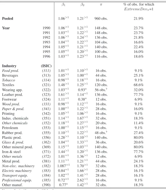
SS,ikt=β1(1−ExtremeDevπ)SD,ikt+β2(ExtremeDevπ)SD,ikt, (13) whereExtremeDevπ is a dummy variable that equals one ifSD,iktbelongs to theπ/2smallest or the π/2 greatest values in the sample and zero otherwise. We testβ1 6= β2 performing Wald tests for several values ofπ, then we consider the larger value of Wald statistic as the most significant break point.18 _Hence,

the estimated critical value ofπsplits the data into three sub-groups: a group of observations that have small values of derived demand deviations, a group of large derived demand deviations, and a group of intermediate derived demand deviations. The two groups of extreme values of demand deviations are of identical size and we assume that the HME is of identical magnitude for both of them. The smaller is the estimated value ofπ the smaller is the size of these two groups of observations. We report in Table5the critical value ofπand the corresponding regression results. The last column in Table5displays the resulting percentage of observations for whichExtremeDevπ= 1, that is the observations for which the slope isβ2.

We first perform this test for the pooled data.19 _{Consistently with the estimations of equation (12) the}

re-sults show evidence of smooth non-linearity (β2> β1>1), which suggests that HME matters for all countries though more strongly for extreme values of demand deviations. When we consider each year successively, we observe a very different result.20 _{The maximum-Wald test identifies a significant break point for aπranking}

from 100 to 148 (i.e. about 20% of the sample). For each year, except 1990 and 1992, β2 is greater than 1 whileβ1 does not statistically differ from 1. Hence, these estimations reveal the presence of a piecewise Home Market Effect (as in Figure 2), and only affect specialization patterns for the first and last decile of country/industry demand deviations. For approximatively 80% of the countries/industries in the sample the estimated production-demand relationship is just proportional.

The remaining lines of Table5report the results for each individual industry.21

According to the maximum-Wald test, the relation between demand and production deviations is strictly linear for two industries only: Wearing apparel (322) and rubber products (355). The results for the latter are clearly consistent with the IRS-MC paradigm. The conclusion for wearing apparel is slightly more ambiguous, but relying upon the value ofβ2, this industry may be classifiable under the CRS-PC paradigm.

For the 23 remaining industry, the Wald test confirms the non-linearity. Seven industries provide unex-pected results. For six of them, bothβ1andβ2are greater than one, butβ1 > β2. These industries exhibit a significant HME and they can be associated to the IRS-MC paradigm, however they do not fit in any of the cases identified in the theoretical model. Note that for all of these industries but beverages the critical values ofπare very high (greater than 120). Therefore, for most countries, the relationship between production and demand deviations show a linear HME with a slope equal toβ1.

Besides these cases, Footwear is the only industry that shows results that are clearly consistent with the CRS-PC paradigm (β1 ≤ 1 andβ2 < β1). Five industries show a smoothly non-linear HME (β1 ≥ 1 and β2> β1). Finally, we observe a piecewise HME for the eleven industries marked by italic font in Table5(i.e. β1= 1andβ2>1).

To sum up, these results show that 16 industries out of 25 exhibit unambiguously the non-linear relation-ship predicted by the model.22 _{More interestingly, considering the eleven industries that exhibit a piecewise}

18_{See Andrews (1993, 2003).}

19_{We increaseπfrom 20 to 2000, using steps of 20 observations.}

20_{There are 625 observations for each year. We preform regressions for values ofπranking from 4 to 624, with a step} of 4 observations.

21_{There are 175 observations for each of the 25 industries. We perform 42 regressions for each of them withπranking} from 4 to 172 with steps of 4 observations.

22_{We also estimated equation (12) considering each industry on its own. The concordance with the results displayed in} table 5 is fairly good, thus we do not report these estimates here (they are available from the authors upon request).