MULTI PARTICLE SWARM OPTIMISATION
ALGORITHM APPLIED TO SUPERVISORY
POWER CONTROL SYSTEMS
by
Abdulhafid Faraj Sallama
Doctor of Philosophy
Department of Electronic and Computer Engineering
College of Engineering, Design and Physical Sciences
Brunel University London
Abstract
Power quality problems come in numerous forms (commonly spikes, surges, sags, outages and harmonics) and their resolution can cost from a few hundred to millions of pounds, depending on the size and type of problem experienced by the power network. They are commonly experienced as burnt-out motors, corrupt data on hard drives, unnecessary downtime and increased maintenance costs. In order to minimise such events, the network can be monitored and controlled with a specific control regime to deal with particular faults. This study developed a control and Optimisation system and applied it to the stability of electrical power networks using artificial intelligence techniques.
An intelligent controller was designed to control and optimise simulated models for electrical system power stability. Fuzzy logic controller controlled the power generation, while particle swarm Optimisation (PSO) techniques optimised the system’s power quality in normal operation conditions and after faults. Different types of PSO were tested, then a multi-swarm (M-PSO) system was developed to give better Optimisation results in terms of accuracy and convergence speed.. The developed Optimisation algorithm was tested on seven benchmarks and compared to the other types of single PSOs.
The developed controller and Optimisation algorithm was applied to power system stability control. Two power electrical network models were used (with two and four generators), controlled by fuzzy logic controllers tuned using the Optimisation algorithm. The system selected the optimal controller parameters automatically for normal and fault conditions during the operation of the power network. Multi objective cost function was used based on minimising the recovery time, overshoot, and steady state error. A supervisory control layer was introduced to detect and diagnose faults then apply the correct controller parameters. Different fault scenarios were used to test the system performance. The results indicate the great potential of the proposed power system stabiliser as a superior tool compared to conventional control systems.
Table of Contents
TABLE OF CONTENTS ... II ACKNOWLEDGEMENTS ... VI DECLARATION ... VII LIST OF ABBREVIATION ... VIII LIST OF FIGURES ... X LIST OF TABLES ... XIV
CHAPTER 1: INTRODUCTION ... 15
1.1 Introduction ... 15
1.2 Motivations ... 16
1.3 Aim and Objectives ... 18
1.4 Challenges ... 18
1.5 Contributions to Knowledge ... 19
1.6 Thesis Outline ... 20
1.7 Author’s Publications ... 23
CHAPTER 2: INTELLIGENT OPTIMISATION SYSTEMS ... 25
2.1 Introduction ... 25
2.2 Optimisation Techniques ... 25
2.2.1 Arithmetic Techniques ... 26
2.2.2 Enumerative Techniques ... 26
2.2.3 Stochastic Search Technique ... 27
2.3 Particle Swarm Optimisation (PSO) ... 27
2.3.1 Classical PSO Algorithm ... 28
2.3.2 PSO Algorithm ... 31
2.4 PSO Derivatives ... 32
2.4.1 Linear Version of Particle Swarm Optimisation (LPSO) ... 32
2.4.2 Global Version of Particle Swarm Optimisation (GPSO) ... 33
2.4.3 Comprehensive Learning Particle Swarm Optimisation (CLPSO) ... 34
2.4.4 Dynamic Multi-Swarm PSO with Local Search (DMS-PSO) ... 34
2.4.5 DMS-PSO with Sub-regional Harmony Search (DMS –PSO- SHS) ... 37
2.4.6 Adaptive Particle Swarm Optimisation (APSO) ... 38
2.4.7 Unified Particle Swarm Optimisation (UPSO) ... 41
2.5 PSO Application in Power Systems ... 42
2.5.2 Economic Dispatch ... 43
2.5.3 Reactive Power and Voltage Control ... 44
2.5.4 Unit Commitment ... 45
2.5.5 Generation and Transmission Planning ... 45
2.5.6 Maintenance Scheduling ... 46
2.5.7 State Estimation ... 47
2.5.8 Model Identification ... 47
2.5.9 Load Forecasting ... 48
2.5.10 Neural Network Training ... 48
2.5.11 Other Applications ... 49
2.6 Summary ... 50
CHAPTER 3: COMBINATION OF MULTI PARTICLE SWARM OPTIMISATION ... 51
3.1 Introduction ... 51
3.2 Combination ... 52
3.3 Empirical Benchmark Functions ... 53
3.3.1 Elliptic Function ... 54 3.3.2 Sphere Function ... 55 3.3.3 Rastrigin’s Function ... 55 3.3.4 Schwefel’s P2.22 Function ... 56 3.3.5 Rosenbrock’s Function ... 57 3.3.6 Ackley’s Function ... 57 3.3.7 Griewank’s Function ... 58 3.4 Comparisons ... 58
3.4.1 Comparison of Algorithms on all Functions ... 59
3.4.2 Comparisons of Each Function on all algorithms ... 63
3.4.3 Algorithms Efficiency Comparisons ... 67
3.5 New Combination of PSOs ... 68
3.5.1 Parallel Structure (PSOs) ... 69
3.5.2 Sequential Structure (PSOs) ... 70
3.6 Experiments ... 73
3.6.1 Experimental Setting ... 73
3.6.2 Comparison of New Method Algorithm on all Functions ... 76
3.6.3 Investigations of the Solution Accuracy ... 76
3.6.4 Comparisons on the Convergence Speed ... 76
3.7 Summary ... 81
4.1 Introduction ... 82
4.2 Control System Stability ... 82
4.3 Relation between Reactive Power Voltage Stability ... 84
4.4 Power System Stability ... 85
4.5 Conventional Control System ... 86
4.6 Power Generators and Power Grid ... 90
4.7 Simulations and Implementation ... 92
4.8 Static VAR Compensator ... 93
4.9 Multi Band Stabiliser ... 94
4.10 Simulation Results ... 95
4.11 Summary ... 97
CHAPTER 5: INTELLIGENT CONTROL AND OPTIMISATION OF POWER SYSTEM STABILISATION... 98
5.1 Introduction ... 98
5.2 Fuzzy Logic Control ... 99
5.3 FPSS Controllers ... 100
5.3.1 Design ... 100
5.3.2 Determining the Scaling Factors ... 103
5.3.3 Membership Function Definition ... 104
5.3.4 Manual Tuning of the Scaling Factors ... 106
5.3.5 Simulation Results ... 107
5.4 Adaptive Neuro Fuzzy Inference System ... 109
5.5 Implementation of ANFIS-PSS Controller ... 111
5.5.1 Training (Single to Three Phases) ... 111
5.5.2 Single Phase Fault Training ... 112
5.5.3 Three Phase-Training ... 116
5.6 ANFIS PSS Response to Ground Fault in Tie Line ... 119
5.6.1 Rotor Speed Deviation on Machine A with (Manual Tuning) ... 119
5.6.2 Rotor Speed Deviation on Machine B with (Manual Tuning) ... 121
5.6.3 Power Quality Control ... 123
5.7 Auto Tuning of Scaling Factors ... 126
5.7.1 Intelligent Optimisation and Cost Function ... 126
5.7.2 Particle Swarm Optimisation ... 127
5.7.3 FLCPSS Auto Tuning ... 127
5.8 Simulation Results ... 128
5.8.2 Rotor Speed Deviation on Machine B with Auto Tuning ... 130
5.8.3 Power Quality Control with Auto Tuning ... 133
5.9 Summary ... 135
CHAPTER 6: SUPERVISORY CONTROL ... 136
6.1 Introduction ... 136
6.2 Supervisory Control ... 137
6.2.1 Hierarchical Supervisory Control ... 138
6.2.2 Optimisation of the Controller ... 140
6.2.3 Fault Detection and Diagnosis ... 140
6.3 System Developments ... 141
6.3.1 Scaled-up Network Power System (Four Generators) ... 141
6.3.2 Controller Auto-Tuning ... 141
6.3.3 Fault Detection System ... 142
6.3.4 Fault Diagnosis ... 144
6.4 Simulation Results ... 145
6.4.1 Scaled-up Model ... 145
6.4.2 Normal Case Simulation ... 147
6.4.3 Multi-Phase Fault ... 148
6.4.4 Fault Scenarios Simulation ... 150
6.4.5 Simulation of Consecutive Serious Fault ... 156
6.5 Summary ... 157
CHAPTER 7: CONCLUSIONS AND FUTURE WORK ... 159
7.1 Conclusions ... 159
7.2 Future Work ... 162
7.2.1 Optimisers ... 162
7.2.2 Neuro Fuzzy Logic System Model ... 163
7.2.3 Benchmarks ... 163
Acknowledgements
All praise is due to Allah (Glorified and Exalted is He), without whose immeasurable blessings and favours (with the prayers of parents, spouse sons and friends) none of this could have been possible.
Firstly I would like to express my sincere appreciation and gratitude to all those who made this thesis possible. This work would not have been possible without help, support and strong motivation of my supervisor, Dr Maysam Abbod, who also gave me the opportunity to work with him in his lab research module and his encouragement, guidance and support from the beginning to the end made my work much easier and more enjoyable.
Also, I would like to express my deepest appreciation to my second supervisor, Prof Gareth Taylor for his important advice and guidance. I will also extend my hand to Late Dr Peter Turner who gave me the first opportunity to work with him in the research lab.
I am heartily thankful to Dr Mohamed Darwish for his support and good spirit which have boosted my moral. I don’t forget Dr Mohammed Ghazi Gronfula who supported me with his knowledge.
I would also like to thank my colleagues especially Basem Alamri, Khaled Sehil, Yaminidhar Bhavanam, Mohammed Alqarni and Shariq Khan who were join me in productive discussions and pushed me to strive towards my goal, and for all their fascinating discussions about the area and the work undertaken.
Lastly, I thank my family for their support, love and encouragement throughout the period. Also I express my sincere thanks to all my teachers, relatives, colleagues, elders and all those from whom I have learnt and gained knowledge.
Declaration
I certify that the effort in this thesis has not previously been submitted for a degree nor has it been submitted as part of requirements for a degree. I also certify that the work in this thesis has been written by me. Any help that I have received in my research work and the preparation of the thesis itself has been duly acknowledged and referenced.
Signature of Student
Abdulhafid Faraj Sallama October 2014, London
List of Abbreviation
Abbreviations Description
AC Alternating Current
AEM Abnormal Event Management
ANFIS Adaptive Neuro-Fuzzy Inference System
ANFIS-PSS Adaptive Neuro-Fuzzy Inference System- Power System Stabilisers
APSO Adaptive Particle Swarm Optimization
BN Big Negative
BP Big Positive
CLPSO Comprehensive Learning Particle Swarm Optimization
COPSS Control And Optimization Of Power System Stabilisation
CPSS Conventional Power System Stabiliser
CPU Central Processing Unit
DE Dispatch Economic
DED Dynamic Economic Dispatch
DGs Distributed Generators
DMS-PSO Dynamic Multi-Swarm Particle Swarm Optimization
DMS-PSO-SHS DMS-PSO With Sub-Regional Harmony Search
EC Evolutionary Computation
ED Economic Dispatch
EP Evolutionary Programing
ES Evolution Strategies
FACTS Flexible Ac Transmission Systems
FDD Fault Detection And Diagnosis
FLC Fuzzy Logic Controller
FLCAT Fuzzy Logic Controller Auto-Trained
FLCMT Fuzzy Logic Controller Manually Tuned
FPSS Fuzzy Logic Controller Power System Stabiliser
GA Genetic Algorithms
GENCOs Generation Expansion Companies
GEP Generation Expansion Problem
GPSO Global Version Of Particle Swarm Optimization
IEEE Institute Of Electrical And Electronic Engineers
LPSO Local Version Of Particle Swarm Optimization
MB-PSS Multiband Power System Stabilizers
MF Membership Function
M-PSO Multi-Swarm Particle Swarm Optimization
N Negative
NF Neuro Fuzzy Logic
NN Neural Network
OPF Optimal Power Flow
OPLF Optimal Power And Load Flow
P Positive
PID Proportional Integral Derivative
PPSO Parallel Particle Swarm Optimisation
PSO Particle Swarm Optimization
PSS2B Power System Stabiliser Type 2B
PSS4B Power System Stabiliser Type 4B
PSSs Power System Stabilisers
Smf S-Shaped Membership Function
SPSO Sequential Particle Swarm Optimisation
SPSSC Supervisory Power System Stability Controller
SPSSC Supervisory Power System Stability Controller
SSMDFLC Supervisory Self-Monitors And Decision Fuzzy Logic Control
STAs Stochastic Technique Algorithms
STS Stochastic Time Series
SVC Static Var Compensator
TSC Thyristor Switched Capacitor
TSR Thyristor Switched Reactor
UPSO Unified Particle Swarm Optimization
VCC Voltage/Var Control
WSM Weighted Sum Method
Z Zero
List of Figures
Figure 1.1: Thesis structure. ... 21
Figure 2.1: Search techniques. ... 26
Figure 2.2: Concept of modification of a searching point by PSO. ... 29
Figure 2.3: General PSO algorithm flowchart. ... 31
Figure 2.4: DMS-PSOs search (J. Liang & Suganthan, 2005). ... 36
Figure 2.5: DMS-PSO sequence. ... 37
Figure 2.6: APSO population distribution information quantified by evolutionary factor f. (Zhan et al., 2009). ... 39
Figure 2.7: Fuzzy membership functions for the four evolutionary states (J. Liang & Suganthan, 2005) ... 40
Figure 3.1: Communication between the optimisers... 53
Figure 3.2: Elliptic function. ... 55
Figure 3.3: Sphere function. ... 55
Figure 3.4: Rastrigin’s function. ... 56
Figure 3.5: Schwefel’s P2.22 function. ... 56
Figure 3.6: Rosenbrock’s function. ... 57
Figure 3.7: Ackley’s function. ... 58
Figure 3.8: Griewank’s function. ... 58
Figure 3.9: Convergence performance of seven test functions on LPSO. ... 59
Figure 3.10: Convergence performance of seven test functions on GPSO. ... 60
Figure 3.11: Convergence performance of seven test functions on CLPSO. ... 60
Figure 3.12: Convergence performance of seven test functions on DMS-PSO. ... 61
Figure 3.13: Convergence performance of seven test functions on DMS-PSO-SHS. ... 61
Figure 3.14: Convergence performance of seven test functions on APSO. ... 62
Figure 3.15: Convergence performance of seven test functions on UPSO. ... 62
Figure 3.16: Convergence performance of seven PSOs on Elliptic function. ... 64
Figure 3.17: Convergence performance of seven PSOs on Sphere function. ... 64
Figure 3.18: Convergence performance of seven PSOs on Schwefel’s P2.22 function. ... 65
Figure 3.19: Convergence performance of seven PSOs on Rosenbrock’s function. ... 65
Figure 3.20: Convergence performance of seven PSOs on Rastrigin’s function. ... 66
Figure 3.21: Convergence performance of seven PSOs on Ackley’s function. ... 66
Figure 3.23: Comparison of the number of internal iteration. ... 69
Figure 3.24: Parallel PSO flowchart. ... 70
Figure 3.25: Serial PSO flowchart. ... 72
Figure 3.26: Comparison of SPSO and PPSO performances using Sphere algorithm. ... 74
Figure 3.27: Comparison of SPSO and PPSO performances using Rosenbrock’s algorithm.74 Figure 3.28: Comparison of SPSO and PPSO performances using Rastrigin’s algorithm. ... 75
Figure 3.29: Comparison of SPSO and PPSO performances using Griewank’s algorithm. .. 75
Figure 3.30: Comparison of new method with other algorithms responses on Elliptic function. ... 78
Figure 3.31: Comparison of new method with other algorithms responses on Sphere function. ... 78
Figure 3.32: Comparison of new method with other algorithms responses on Schwefel’s P2.22 function. ... 79
Figure 3.33: Comparison of new method with other algorithms responses on Rosenbrock’s function. ... 79
Figure 3.34: Comparison of new method with other algorithms responses on Rastrigin’s function. ... 80
Figure 3.35: Comparison of new method with other algorithms responses on Ackley’s function. ... 80
Figure 3.36: Comparison of new method with other algorithms responses on Griewnak’s function. ... 81
Figure 4.1: Time frame of the basic power system dynamic phenomena (Machowski et al., 2011). ... 83
Figure 4.2: A simplified model of a network element. (a) equivalent diagram and phasor diagram; (b) real power and reactive power characteristics (Machowski et al., 2011). 84 Figure 4.3: Classification of power system stability (Machowski et al., 2011). ... 86
Figure 4.4: CPSS diagram. ... 87
Figure 4.5: Block diagram of excitation control system. ... 91
Figure 4.6: Block diagram of the simulated Matlab power system toolbox (Larsen & Swann, 1981). ... 93
Figure 4.7: Single-line diagram of an SVC. ... 94
Figure 4.8: Conceptual block diagram of the multiband PSS (IEEE PSS4B). ... 95
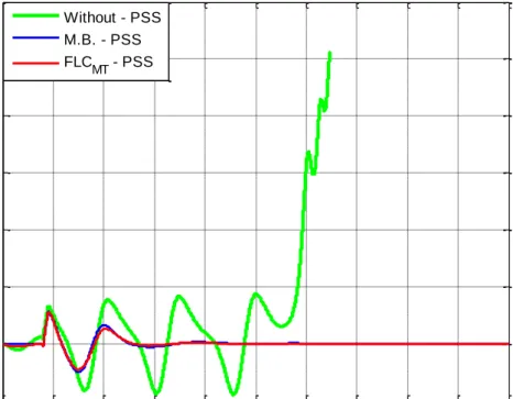
Figure 4.9: Multi-band stabiliser response comparing with PSS2B and without PSSs during fault in one phase... 96
Figure 4.10: Multi-band stabiliser response comparing with PSS2B and without PSSs during
fault in two phases. ... 96
Figure 4.11: Multi-band stabiliser response comparing with PSS2B and without PSSs during fault in three phases. ... 97
Figure 5.1: Two generators connected together in a small network. ... 100
Figure 5.2: Generalized FLC auxiliary fuzzy controller and Structure of FLC. ... 101
Figure 5.3: Membership functions for inputs and output fuzzy sets of the FLC. ... 102
Figure 5.4: Control surface of ANFIS-based FPSS controller. ... 103
Figure 5.5: Block diagram for FLC controller. ... 103
Figure 5.6: Gaussian membership functions. ... 105
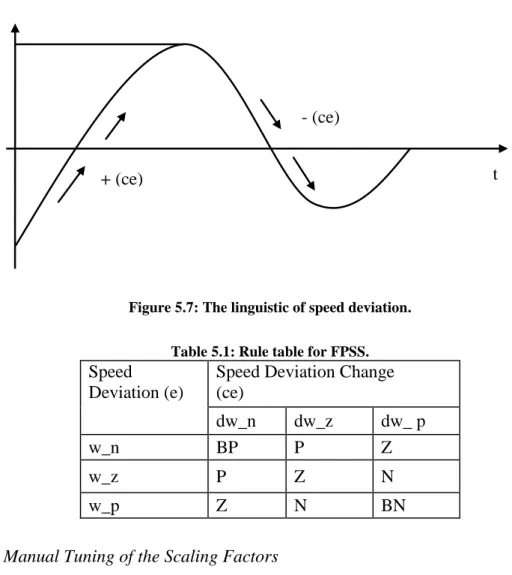
Figure 5.7: The linguistic of speed deviation. ... 106
Figure 5.8: System behaviours during one phase fault Simulation results. ... 107
Figure 5.9: System behaviours during two phase fault simulation results. ... 108
Figure 5.10: System behaviours during three phase fault simulation results. ... 108
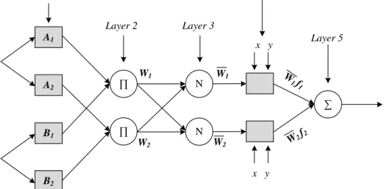
Figure 5.11: A typical ANFIS architecture (Schwefel, 1981). ... 109
Figure 5.12: FLC training in ANFIS editor. ... 113
Figure 5.13: ANFIS editor parameters. ... 113
Figure 5.14: System’s response to one phase fault with single phase training. ... 114
Figure 5.15: System’s response to two phase faults with single phase training. ... 115
Figure 5.16: System’s response to three phase faults with single phase training. ... 115
Figure 5.17: FLC training in ANFIS editor. ... 117
Figure 5.18: System’s response to one phase fault with three phase training. ... 117
Figure 5.19: System’s response to two phase faults with three phase training. ... 118
Figure 5.20: System’s response to three phase faults with three phase training. ... 118
Figure 5.21: Rotor speed deviation at Machine A for one phase fault... 120
Figure 5.22: Rotor speed deviation at Machine A for two phase fault. ... 120
Figure 5.23: Rotor speed deviation at Machine A for three phase fault. ... 121
Figure 5.24: Rotor speed deviation at Machine B for one phase fault. ... 122
Figure 5.25: Rotor speed deviation at Machine B for two phase fault... 122
Figure 5.26: Rotor speed deviation at Machine B for three phase fault. ... 123
Figure 5.27: System behaviours during one phase fault. ... 124
Figure 5.28: System behaviours during two phase fault. ... 124
Figure 5.29: System behaviours during three phase fault. ... 125
Figure 5.31: System behaviours during two phase fault. ... 129
Figure 5.32: System behaviours during three phase fault. ... 130
Figure 5.33: System behaviours during one phase fault. ... 131
Figure 5.34: System behaviours during two phase fault. ... 132
Figure 5.35: System behaviours during three phase fault. ... 132
Figure 5.36: System behaviours during one phase fault. ... 133
Figure 5.37: System behaviours during two phase fault. ... 134
Figure 5.38: System behaviours during three phase fault. ... 134
Figure 6.1: Supervisory block diagram. ... 139
Figure 6.2: Single line diagram of the scaled-up power system. ... 141
Figure 6.3: Flowchart of fault diagnosis for power system network. ... 143
Figure 6.4: Matlab/Simulink Block diagram of the scaled-up power system. ... 146
Figure 6.5: System response to normal operation with 3-phase training and auto-tuning. .. 147
Figure 6.6: System’s response to 1-phase fault with 3-phase training and auto-tuning. ... 148
Figure 6.7: System’s response to 2-phase fault with 3-phase training and auto-tuning. ... 149
Figure 6.8: System’s response to 3-phase fault with 3-phase training and auto-tuning. ... 150
Figure 6.9: System’s response to normal operation with comparison supervisory control, MB and Generic PSS. ... 151
Figure 6.10: System’s response to fault 1 with comparison supervisory control, MB and Generic PSS. ... 151
Figure 6.11: System’s response to fault 2 with comparison supervisory control, MB and Generic PSS. ... 152
Figure 6.12: System’s response to fault 3 with comparison supervisory control, MB and Generic PSS. ... 153
Figure 6.13: System’s response to fault 4 with comparison supervisory control, MB and Generic PSS. ... 153
Figure 6.14: System’s response to fault 5 with comparison supervisory control, MB and Generic PSS. ... 154
Figure 6.15: System’s response to fault 6 with comparison supervisory control, MB and Generic PSS. ... 155
Figure 6.16: System’s response to fault 7 with comparison supervisory control, MB and Generic PSS. ... 156
List of Tables
Table 3.1: Benchmark functions, uni-modal and multi-modal. ... 54
Table 3.2: Comparison performance of seven PSOs algorithms on seven benchmark functions. ... 63
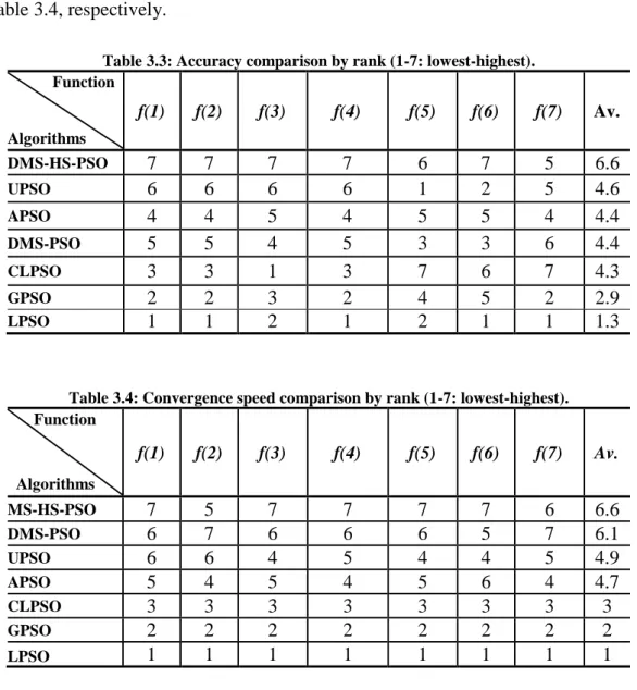
Table 3.3: Accuracy comparison by rank (1-7: lowest-highest). ... 68
Table 3.4: Convergence speed comparison by rank (1-7: lowest-highest). ... 68
Table 3.5: Mean and standard deviation results for the 7 benchmark functions using different PSO types. ... 77
Table 5.1: Rule table for FPSS... 106
Table 5.2: Manual tuning of the FLC scaling factors. ... 106
Table 5.3: Simulation results for three phase fault with single phase training. ... 116
Table 5.4: Simulation results for three phase fault with three phase training. ... 119
Table 5.5: Speed deviation response for three phase fault with three phase training (Machine B). ... 121
Table 5.6: Simulation results for three phase fault with three phase training. ... 125
Table 5.7: Final value for auto-tuning scaling factor. ... 127
Table 5.8: Speed deviation response for three phase fault with three phase training and auto tuning (Machine A). ... 128
Table 5.9: Speed deviation response for three phase fault with three phase training. and auto tuning (Machine B). ... 131
Table 6.1: Final auto-tuning scaling factor values. ... 142
Table 6.2: Fault diagnosis rule basis values. ... 145
Table 6.3: Simulation results for multi fault with auto-tune and M-training. ... 149
Chapter 1:
Introduction
1.1Introduction
Power system stabilisers (PSSs) have been utilized for decades to deliver damping to system oscillations. Local, conservatively distributed local PSSs (LPSSs) are deliberated to have fixed parameters gathered from a stabilised model around a certain operating point. Final configurations are prepared by field tests at one or two operating points. A major source of model fluctuation and disturbance can be caused by the inherent nonlinearity in the system. Power systems operate in a changing and highly non-linear environment as a result of change in loads, key operating parameters and generator output. When the system is exposed to a disturbance, the stability of the system will be a subject of the nature of the disturbance as well as the initial operation condition (Kundur et al., 2004).
In this thesis, the term uncertainty concerns the lack of precision in modelling of all elements in electrical power grid containing the transformers, the transmission lines, and the loads, in addition to the fluctuation of clear linearized power plant control factors as the operating point fluctuates. LPSS parameters based on any single model are probably not optimal and may limit the linearizing impact. Nonetheless, in the developed system negligible errors can be minimised, particularly if the damping controller is designed on the basis of the robustness standards and the closed-loop system preserves an acceptable performance level. Some modifications should be applied to the system of power system controllers, particularly PSSs utilising Optimisation techniques in the case of disturbances and failures (Snyder et al., 1999) (Klein et al., 1995) . The likelihood of strong coupling among the local modes and the interarea modes would render the tuning of LPSSs for damping all modes nearly unachievable when there is no supervisory level controller. The intelligent system has been utilised to organise multiple local controllers in electrical power system (Guo, Hill, & Wang, 2001).
Intelligent systems are tools and methodologies inspired by nature to solve computationally intensive problems in mathematics that are very important for the progress of current trends in survey and information technology. Artificially intelligent systems these days utilize computers to be easily emulate various
biological metaphors and faculties of human intelligence. They use techniques which combine the symbolic and sub-symbolic systems capable of developing human knowledge abilities and intelligence, not merely to do things that humans can do well. Intelligent systems are ideally suited for tasks s9uch as optimisation and search, pattern recognition and adaptation, planning, vagueness management, control and adjustment. In this thesis, the technologies of intelligent systems and their implementation are highlighted by a series of examples.
In the domain of artificial intelligence, neuro fuzzy logic (NF) denotes combinations of fuzzy logic and artificial neural networks. NF systems use a self-learning algorithm derived and inspired by the concept of neural networks to achieve the use of processed data samples (their fuzzy sets and fuzzy rules) (J. Jang, 1993a). However, in this research using this methodology to develop stability control system is integrated with an Optimisation methodology such as particle swarm Optimisation (PSO) (Kennedy & Eberhart, 1995b) to determine the optimum supervisory control parameters. Furthermore, an accurate electrical stability control system element model adapted for fast response, overshooting, fluctuation and to eliminate the steady state error was developed using standard data for Optimisation purposes.
This research explores different types of Particle Swarm Optimisation (PSO) as intelligent Optimisation methodologies for the purpose of emphasis on the application to tune the power stability control elements and hierarchical control systems. Different types of PSOs give different Optimisation results in terms of accuracy and convergence speed. The advantage of the ones characterises in quick convergence and low accuracy can be combined with those that have slow convergence but accurate results. The new algorithm will be a combination of fast and accurate optimisers such that the benefit of both system are utilised. The developed optimiser can be tested on different benchmark.
1.2Motivations
The motivation for this thesis is two-fold:
First, the need for evolutionary algorithms to optimise nonlinear or change state frequently problems. Scaling the possibility of Optimisation algorithm programs to find the best solutions for that type of complex problems via using computing
systems and high-tech solutions whereby evolutionary algorithms are applied to solve static problems; however, many real-world systems are often continuous or change state frequently. The system state changes necessitate recurrent (sometimes frequent or continuous) re-Optimisation. It has been shown that the Optimisation of the particle swarm can be applied successfully for dynamic control and optimisation systems (Eberhart & Shi, 2001a). Therefore, there is great need for an efficient algorithm that is able to solve real, complex, multi-dimension problems. In fact to develop such an algorithm, several models have to be developed, such as different types of PSO optimisers, and appropriate benchmark functions should be selected to test new algorithm and power system stability control with supervisory control in electrical network.
This thesis presents intelligence algorithms capable of dealing with the intricacy of electrical power system problems using PSOs algorithm methodologies, which are considered to be robust adaptive Optimisation techniques. Furthermore, an effective algorithm based on algorithms portfolio procedure can be developed using different types of PSOs algorithms techniques whereby the communication between these algorithms in the early stages can be considered (the fast and less accurate algorithm can pass its results to the slow and more accurate algorithm, which will consequently benefit from the good results at an early stage).
Second, the electrical power energy market is evolving with the progressive growth of networks and a continuous improvement in performance, rapidly increasing the number of consumers and the critical need for sophisticated control equipment governing generation plants to produce high quality energy in terms of continuity, stability, reliability, flexibility and quick response. Furthermore, the rapid development in the use of the solar panels, wind turbines and other sustainable energy sources, which are mostly turbulent and unpredictable sources, requires advanced control devices.
Steady state stability or power transient is defined as the ability of a power system to control stably without loss of synchronisation between power plant generations after a small or large disturbance. Moreover, voltage stability is the system ability to maintain load voltage magnitudes under steady state conditions within specified operating limits. Since it has become increasingly difficult to obtain power plant sites
in the vicinity of power consumers (due to the lack of space for large power facilities in urban areas and public opposition to power infrastructure), electrical power is now often transported over long distances using large capacity lines. Under these circumstances, voltage stability can be a major problem, as well as transient and steady state stabilities (Abe, Fukunaga, Isono, & Kondo, 1982).
1.3Aim and Objectives
The overall aim of the thesis is to introduce and design a new controller device working on the principle of neurons fuzzy logic and artificial intelligence, using a new Optimisation algorithm as a novel paradigm in the stability and supervision of electrical network.
The research aim is addressed through the following objectives:
1. To review the area of searching techniques and intelligent Optimisation algorithms.
2. To review different types of PSOs algorithms as stochastic swarm intelligence technique.
3. To review different types of linear and non-linear functions to be used as benchmark.
4. To introduce new combination of multi particle swarm Optimisation paradigm. 5. To review power system stability and the most important devices currently used
for this purpose.
6. To apply the new intelligent Optimisation algorithm in power system stability. 7. To scale-up the control system and development a new supervisory stability
control system. 1.4Challenges
There are many technical challenges in developing the control device and supervision of the electrical power system by the use of artificial intelligence technique. These challenges are inherited from the original components of stability control with the following considerations:
In real-world applications, optimising problems is much more complex because of various constraints, objectives and the size of the search space involved, in relation to different types of controlling.
There is a need to develop a system that is able to control electrical power system stability in networks with high-quality continuity, stability, reliability, flexibility and quick response.
Stability control system should handle any phenomenon causing instability in the electrical network using artificial intelligent techniques.
An efficient electrical network containing fuzzy logic controller model administrating stability can be used for Optimisation purposes.
There is a need for an efficient algorithm that can solve and optimise the parameters problems of multi controller network.
A suitable technique should measure the quality of multiple objectives.
A new PSOs technique that can guarantee feasible solutions is needed.
A hierarchical control system should detect the system frailer and find immediate solutions using new Optimisation algorithm and artificial intelligent paradigm.
1.5Contributions to Knowledge
This research developed a multi PSO intelligent Optimisation program. This algorithm includes a combination of different types of PSOs, such as Local Version of Particle Swarm Optimisation (LPSO), Global Version of Particle Swarm Optimisation (GPSO), Dynamic Multi-Swarm Particle Swarm Optimisation DMS-PSO with Sub-regional Harmony Search (DMS-DMS-PSO-SHS), Adaptive Particle Swarm Optimisation (APSO) and others. Moreover, an effective paradigm was developed using all previous algorithms based on portfolio methodology in two patterns, parallel and serial. In this manner of communication between different algorithms is considered in the early stages, whereby the fast convergence and less accurate algorithm can pass its results to the slow and more accurate algorithm, which will benefit from the good results at an early stage.
Moreover, a number of different types of benchmark functions evaluate each algorithm individually, and the results can be compared together in addition to the
new optimal algorithm. This analytical technique enables identification of the best paradigm to discover the different crossover effects and a practical manner to avoid the generation of useless solutions in extensive systems.
A fuzzy logic controller model was developed and auto tuned for Optimisation purposes. This model provides a new stability controller type, using NF and PSO procedures as expression of artificial intelligence to optimise the controller scale of factors. Subsequently, an altogether successful model of an advanced control system was developed.
The intelligent supervisory system that is able to control stability in electrical network when facing any disturbances and during normal operation with high efficiency in power quality causes the least trouble for consumers. This system deals with multiple objectives and measures the fitness of each solution that is generated by the system. The system used Weighted Sum Method (WSM) techniques and the hierarchy technique to address the problem of the stability control in hierarchy promised stages.
1.6Thesis Outline
The work presented in this thesis is organised into seven chapters. Figure 1.1 illustrates the structure of the thesis and relationship to the thesis objectives presented in section 1.3.
Chapter 1
Introduction
Chapter 2
Intelligent Optimisation Systems
( Objective 1 & 2)
Chapter 7
Conclusions and Future work
Chapter 4
Power System Stabilisation ( Objective 5)
Chapter 5
Intelligent Control on Power System Stabilisation ( Objective 6) Chapter 6 Supervisory Control ( Objective 7) Chapter 3
Multi Particle Swarm Optimisation ( Objective 3 & 4)
Background
Design
Figure 1.1: Thesis structure.
Following this introductory chapter, the next six chapters contain more detailed information about the theoretical background and technical development of artificial intelligent and power stability devices.
Chapter 2 presents a detailed background about intelligent Optimisation systems and their evolution. It explores how Optimisation tools have become an important part of life to solve constrained and unconstrained continuous and discrete problems, by providing generic algorithms as part of stochastic techniques. The chapter reviews and compares related paradigms intelligent research methods. The chapter concludes with a brief summary and discussion.
Chapter 3 introduces the combination of MPSO and outlines a group of complex functions to be used in benchmark testing. A new method is proposed using different Optimisation schemes which are combinations of different types of PSO and methods used simultaneously, to make use of the characteristics of each individual method to tackle the same problem. The proposed schemes can utilize and share information about the local and global best as well as the swarm population, in specific predefined iteration of all types simultaneously.
Chapter 4 lays the background for power system stabilisation by presenting the resource scheduling problem and the latest conventional device in this area. This chapter presents power system stability by discussing the most important four dynamic phenomena affecting it, namely wave, electromagnetic, electromechanical and thermodynamic phenomena. Furthermore, the relationship between reactive power voltage and stability is explored; this variable is one of the most important targets in the search, as an actual variable that indicates the state of the electrical power grid in terms of stability. Additionally, this chapter, through mathematical analysis, discusses the most important types of power system stability devices to learn the working methods, as well as tuning methods. The most important faults types which affect the power system stability of the electrical grid are then described, allowing with how these problems can be emulated by software programs for the purpose of analysis. Finally, the latest types of conventional power system stabiliser (PSS4B) devices are explained and tested using different conditions and compared to other devices from prior generations.
Chapter 5 applies the intelligent control and Optimisation on the power system stabilisation. Furthermore to describes the current state of the intelligent Control and Optimisation of Power System Stabilisation (COPSS). Furthermore, it explains the fuzzy logic controller and the design and tune stable control system using fuzzy logic controller before the specific approach in neuro fuzzy logic systems. The implementation of ANFIS-PSS controller and training them in different stages is described, involving single- and three-phase training. The new ANFIS-PSS controller response to ground fault in tie line in machines A and B is then explained and the power quality in the network is outlined before the auto tuning of scaling factors using intelligent Optimisation, and the simulation results of rotor speed
deviation on both machines A and B, in addition to comparing the power quality in the network.
Chapter 6 introduces in detail a new supervisory control describing the design and implementation of advanced Supervisory Power System Stability Controller (SPSSC) using neuro-fuzzy system and Matlab S-function tool, whereby the controller is taught from data generated by simulating the system for the optimal control regime. The controller is compared to a multi-band control system which is utilized to stabilize the system for different operating conditions. Simulation results show that the supervisory power system stability controller produced better control action in stabilizing the system for conditions such as: normal, after disturbance in the electrical grid as a result of changing of the plant capacity like switching renewable energy units, high load reduction or in the worst case of fault in operating the system, e.g. phase short circuit to ground. The new controller decreased the settling time and overshoot after disturbances, which means that the system can reach stability in the shortest time with minimum disruption. Such behaviour improves the quality of the provided power to the power grid.
Chapter 7 summarises the thesis aims, major contributions and significant findings. It highlights areas and directions for further research.
1.7Author’sPublications
A number of journal and conference papers related to this thesis have been published at international conferences and in journals, and some recent additional papers are pending acceptance for international conferences and journals, as presented below.
A.Conference papers (Published)
[1] A. Sallama and M. Abbod, “Neuro-Fuzzy System for Power Generation Quality” published on ISGT 2011, December 2011.
[2] A. Sallama, M. Abbod, P. Turner, “Neuro-Fuzzy System for Power Generation Quality Improvements” published on UPEC 2012, Brunel University, September 2012.
[3] A. Sallama, M. Abbod, P. Turner, “Intelligent Control System for Power System Stability” published on ResCon 2012, Control Engineering , Power System Second year of PhD.
[4] A. Sallama, M. Abbod, G Taylor, “ Development Intelligent Control System for Power System Stability” published on ResCon 2013, Control Engineering , Power System third year of PhD.
[5] A. Sallama, M. Abbod, P. Turner, “Supervisory Power System Stability Control Using Neuro-Fuzzy System and Particle Swarm Optimisation Algorithm” published on UPEC 2014, Technical University of Cluj-Napoca, Romania, September 2014.
B.Conference papers (Accepted)
[6] B. Alamri, A. Sallama, M. Darwish, “Optimum SHE for cascaded H-Bridge multilevel inverter using: NR-GA-PSO, comparative study” ACDC 2015, The 11th International Conference on AC and DC Power Transmission,10 - 12 February 2015, Birmingham, UK.
C.Journal papers (Published)
[7] Sallama and M. Abbod, "Applying Sequential Particle Swarm Optimisation Algorithm to Improve Power Generation Quality", International Journal of Engineering and Technology Innovation, 2014.
D.Journal papers (Accepted)
[8] Shariq Mahmood Khan, R.Nilavalan, Abdulhafid Sallama, “A Novel Approach for Reliable Route Discovery in Mobile Ad-Hoc Network” Wireless Personal Communications, October 2014.
Chapter 2:
Intelligent Optimisation Systems
2.1Introduction
Optimisation tools are becoming increasingly important in everyday life to solve constrained and unconstrained, continuous and discrete problems, by providing widely algorithms as part of stochastic technique algorithms (STAs), which are very effective in solving standard and large-scale Optimisation problems (Mahfoud, 1995), provided that the problem does not require multiple solutions (e.g. classification problems in machine learning where, in single run, multiple optima and peaks need to be found) (Koper, Wysession, & Wiens, 1999).
2.2Optimisation Techniques
Optimisation has been an active area of research for several decades. As many real-world Optimisation problems become increasingly complex, better Optimisation algorithms are always needed. Unconstrained Optimisation problems can be formulated as n dimensional minimization, thus:
𝑀𝑖𝑛 𝑓(𝑥), 𝑥 = [𝑥1, 𝑥2, … . . , 𝑥𝑛] (2.1)
where n is the number of the parameters to be optimized.
In case of searching for optimum solutions, using Optimisation techniques there are three main broad classes used to find the solution mentioned by Goldberg (Goldberg, 1990), as shown in Figure 2.1. The following subsections list the different types of Optimisation technique with a short description of each.
Arithmetic techniques Stochastic technique Enumerative techniques Search Techniques Indirect Methods Direct Methods Evolutionary Algorithms Simulated Annealing Dynamic Programming Newton Swarm Intelligence Evolutionary Strategies Bee Bacterial Growth Fibonacci Animal Herding PSOs Ant Colonies Genetic Algorithms Genetic Programming Firefly
Figure 2.1: Search techniques.
2.2.1 Arithmetic Techniques
Arithmetic techniques can be divided into two types: direct and indirect. Direct ways, such as those of Newton and Fibonacci (Bóna, 2011), seek the greatest "jump" on the search space and evaluate the gradient of a new point approaching the solution. Indirect ways are conducted by solving a set of non-linear equations to search for local extreme values, typically caused by a gradient of the objective function equal to zero, and by restricting itself to points to search for possible solutions (function peaks) with zero slope in all directions.
2.2.2 Enumerative Techniques
This technique is very simple to implement, requiring high significance computation applied on applications with too large a domain space, because every point search to an objective function's at domain space (Ribeiro Filho, Treleaven, & Alippi, 1994). A good example for that technique is a dynamic programming.
2.2.3 Stochastic Search Technique
In this case, search techniques are based on enumerative techniques in addition to using more essential information to guide the random search processing. This is done by three major methods: evolutionary algorithms, intelligent swarm and simulated annealing. Intelligent algorithms use natural selection principles or simulate the natural particle swarm as in bird flocking or fish school phenomena (Kennedy, Kennedy, & Eberhart, 2001). Here, the solutions are improved features of possible solutions throughout generations by biological processes inspired in such techniques. Particle swarm Optimisation (PSO) and genetic algorithms (GA) are good examples for this technique. Simulated annealing used a thermodynamic evolution process to search for possible solutions (Schwefel, 1981).
2.3Particle Swarm Optimisation (PSO)
Most creatures in nature behave as swarms. The study of artificial life is highly influenced by studies of natural swarm behaviour, which has been mapped and reconfigured in mathematical models which can be processed by computers (Liu & Passino, 2000). PSO mathematically requires only primitive mathematical operators that can be implemented by computer models and code in a few lines. This feature makes it inexpensive in terms of both memory and speed requirements. Furthermore, the PSO has been known as evolutionary computation technique (Kurian, George, Bhat, & Aithal, 2006a) , and have all the features of Evolution Strategies (ES), Genetic Algorithms (GA) and Other evolutionary computation (EC) techniques, such as utilizing some searching points in the solution space, similar to genetic algorithms (Eberhart & Shi, 1998) (Panduro, Brizuela, Balderas, & Acosta, 2009).
A GA system is initialized with a population of random solutions. While GA can handle combinatorial Optimisation problems, PSO has continuous Optimisation problems. In contrast to GA, each single population is also assigned a random speed in PSO, in effect to flying them through the solution hyperspace. Moreover, PSO has been enhanced in the combinatorial Optimisation problems, thus it is possible to simultaneously search the optimal solution in several dimensions, unlike other evolutionary computation techniques (Tandon, El-Mounayri, & Kishawy, 2002).
Several scientists (e.g. Heppner and Grenander, 1990; Reynolds, 1987) studied a particularity of synchronized movement without collision for the members of bird flocks and fish schools. Eberhart and Kennedy (1995) developed new evolutionary computation technique dubbed PSO, and Shi and Eberhart (1996) introduced the concept of inertia weight to the original version of PSO, in order to improve the search during the Optimisation process (Shi & Eberhart, 2001)(Eberhart & Shi, 2001b). Several types of developed PSO subsequently emerged, as explained in this section, in addition to the updated types such as those devised during this research. 2.3.1 Classical PSO Algorithm
PSO developed as a simulation of the bird flocking flow, in two space dimensions (x, y), where (vx) represents the agent velocity in the direction of x-axis, (vy) represents the agent velocity in the direction of y-axis, (x, y) represents the agent’s current position and (vx, vy) represents the current velocities in two dimensions. From the
velocity and position information, the agent can be modified for the new position. The school of fish and birds flock optimizes a given objective function based on the experiences and every time solution. The particle recognizes this information and an analogy is stored each time in under the name of the local best solution (pbest). At the same time in every cycle all particles recognize the best solution for all groups stored each time under the name of the global best solution (gbest). Depending on this information, each particle recognizes its performance, and performs in tandem with all other particles in the group. Therefore, each particle tries to adjust its position as shown inFigure 2.2, using the following information:
Current positions (x, y),
Current velocities (vx, vy),
Distance between the current position (x, y) and pbest
Figure 2.2: Concept of modification of a searching point by PSO.
where
Sk: current searching point. Sk+1: modified searching point. Vk: current velocity.
Vk+1: modified velocity.
Vpbest: velocity based on pbest. Vgbest: velocity based on gbest
From the concept of velocity the new position is represented and modified (i.e. the modified value for the current positions). The following equation 2.2 by (Eberhart & Shi, 1998) expresses the modified velocity of each particle:
𝑉𝑖𝑘+1 = 𝑊𝑉
𝑖𝑘+ 𝑐1𝑟𝑎𝑛𝑑1× (𝑝𝑏𝑒𝑠𝑡𝑖 − 𝑆𝑖𝑘) + 𝑐2𝑟𝑎𝑛𝑑2× (𝑔𝑏𝑒𝑠𝑡𝑖 − 𝑆𝑖𝑘) (2.2 ) where
Vik+1: velocity of particle i at iteration k+1.
Vik: velocity of particle i at iteration k.
W: inertia function.
C1 and C2: are the acceleration constants.
Rand1 and Rand2: random number between 0 and 1. Sik: current position of particle i at iteration k.
Vk+1 X Y Sk Vk Vpbest Vgbest Sk+1
pbesti: best position of particle i.
gbest: the global best position of the group.
While the inertia weighting function is usually utilized as follows:
𝑊 = 𝑊𝑚𝑎𝑥 −
𝑊𝑚𝑎𝑥 − 𝑊𝑚𝑖𝑛
𝑖𝑡𝑒𝑟𝑚𝑎𝑥 × 𝑖𝑡𝑒𝑟𝑖 (2.3) where
Wmax: initial weight, Wmin: final weight,
itermax: maximum iteration number. iteri: current iteration number.
Equation 2.2 can be explained as follows. The RHS of consists of three terms, the first of which is the previous velocity of the particle. The second and third terms are utilized to change the velocity of the particle. Without the second and third terms, the agent will keep on “flying” in the same direction until it hits the boundary (i.e. it tries to explore new areas). Therefore, the first term corresponds to the diversification in the search procedure. On the other hand, without the first term, the velocity of the “flying” particle is only determined by using its current position and its best positions pbest in history. The particles will try to converge in the pbests and/or gbest, therefore the terms are corresponding to intensification in the search procedure (Eberhart & Shi, 2001b).
Figure 2.2 illustrates a concept of modification with particles in the solution space. Each particle finds the new position using the integration of velocity vectors. The current position can be modified by the following equation:
𝑆𝑖𝑘+1 = 𝑆𝑖𝑘+ 𝑉𝑖𝑘+1 (2.4)
where
Sk+1: modified searching point. Sk: current searching point. Vk+1: modified velocity.
2.3.2 PSO Algorithm
PSO algorithm comprises a very simple concept, and paradigms are implemented in a few lines of computer code. The general flow chart of PSO is shown in Figure 2.3 and described below:
Start
Generation of initial population
Modification of particles speed and position
Evaluation of searching point of each Particle Max. iteration reached End Yes No Step 1 Step 4 Step 3 Step 2
Figure 2.3: General PSO algorithm flowchart.
Step 1:Generate initial condition for each agent. Initial position searching points of particle i at iteration k = 0, (Sik) and velocities (Vik) of each agent are usually generated randomly within the allowable range. The current searching point is set to pbest for each agent. The best-evaluated value of pbest is set to gbest and the agent number with the best value is stored.
Step 2: Evaluation of searching point of each particle. The objective function value is calculated for each particle. If the obtained value is better than the current local best value pbest of the particle, the new pbest value is replaced by the current value. If the local best value of pbest is better than the current global best value gbest, then
the new gbest is replaced by the best value and the particle number with the best value is stored.
Step 3: Modification of each searching point Sk+1. The current searching point Sk of each particle updated using previous equations 2.2 and 2.4.
Step 4: Checking the exit condition. The current iteration number reaches the predetermined maximum iteration number, then exit. Otherwise, go to step 2.
The detailed features of the searching procedure of PSO are:
(I). As shown in equations 2.2 and 2.4, PSO can essentially handle continuous Optimisation problem.
(II). Similar to GA, the PSO utilizes several searching points and the searching points gradually get close to the optimal point using their local best pbests and the global best gbest.
(III). The first term of right-hand side at equation 2.2 corresponds to diversification in the search procedure. The second and third terms at RHS of the equation correspond to intensification in the search procedure. This method has a well-balanced mechanism to utilize diversification and intensification in the search procedure efficiently.
(IV). The above concept of PSO can use more than two dimensions in the space. However, the method can be easily applied to n-dimension problem. In other words, PSO can handle continuous Optimisation problems with continuous state variables in an n-dimension solution space.
2.4PSO Derivatives
As mentioned earlier in this chapter, PSO is one of the most important groupings under swarm intelligence, but it in turn is divided into several types, the most important of which are explained below.
2.4.1 Linear Version of Particle Swarm Optimisation (LPSO)
In the linear version of PSO, the particles are not influenced by random strangers; they are only affected by their topological neighbours. The topological geometry of
the particle swarm remains constant throughout the run. It is sometimes called local PSO (LPSO). LPSO is much like classical PSO, except that rather than use a different random number for each element of the velocity and position vectors, a single scalar is multiplied by each vector, thus:
𝑉𝑡+1= 𝑤𝑣𝑡+ ∅1𝑈1𝑡(𝑝𝑖− 𝑥𝑡) + ∅2𝑈2𝑡(𝑔𝑖− 𝑥𝑡) (2.5)
where w is the inertia weight, each Ø1,2 ≈ 2, and U1,2 is a vector of numbers drawn
from a standard uniform distribution.
This means that the resultant velocity (and therefore position) is a strictly linear combination of other particle positions. If the particles are all initialized within
𝑓 = {𝑥|𝐴𝑥 = 𝑏}, then they will always be within f (Mendes, Kennedy, & Neves,
2004).
2.4.2 Global Version of Particle Swarm Optimisation (GPSO)
GPSO first introduced a new parameter called inertia weight into the original particle swam optimiser in order to increase the performance of the PSO. Initial GPSO found that inertia weight in the range (0.9, 1.2) on average will have a better performance; that is, it has a bigger chance to find the global optimum within a reasonable number of iterations (Yuhui Shi & Eberhart, 1998). Furthermore, a time decreasing inertia weight is introduced which brings in a significant improvement on the PSO performance as in (Zhan & Zhang, 2008); this research approved that the best value of inertia weighting during the Optimisation should be change from minimum value 0.4 to maximum value 0.9 (Shi & Eberhart, 1998), (Eberhart & Shi, 2001c) linked to this equation:
𝑤 = 𝑤𝑚𝑎𝑥− (𝑤𝑚𝑎𝑥− 𝑤𝑚𝑖𝑛
𝐺 ) × 𝑔 (2.6)
where
Wmax: maximum value of inertia weight, Wmin: minimum value of inertia weight, G: maximum iteration number,
In GPSO, each particle’s velocity is adjusted according to its personal best and the performance achieved so far within learning from the personal best and the best position achieved so far by the whole population; instead of the local version each particle’s velocity is adjusted according to its personal best and the performance achieved so far within its neighbourhood.
2.4.3 Comprehensive Learning Particle Swarm Optimisation (CLPSO)
CLPSO utilizes a novel learning strategy pattern whereby all other particles’ historical best information, is used to update a particle’s velocity. This strategy enables the diversity of the swarm to be preserved to discourage premature convergence.
In this strategy, the following equation is used to update the velocity:
𝑉𝑖𝑑 ← 𝑤 ∗ 𝑉𝑖𝑑 + 𝑐∗ 𝑟𝑎𝑛𝑑
𝑖𝑑∗ (𝑝𝑏𝑒𝑠𝑡𝑓𝑖(𝑑)𝑑 − 𝑋𝑖𝑑) (2.7) where d the dimension and i the particle
𝑐∗: are the acceleration constants,
𝑉𝑖𝑑 : the velocity,
𝑋𝑖𝑑: the position, W: inertia function.
𝑓𝑖 = [ 𝑓𝑖(1), 𝑓𝑖(2), . . . . 𝑓𝑖(𝐷)]: defines of pbest’s which particle i should be
followed.
𝑝𝑏𝑒𝑠𝑡𝑓𝑖(𝑑)𝑑 : can be the corresponding dimension of any particles.
2.4.4 Dynamic Multi-Swarm PSO with Local Search (DMS-PSO)
The dynamic multi-swarm particle swarm optimiser, where is constructed based on the basic version of PSO and a new neighbourhood topology, is used in this case (J. Liang & Suganthan, 2005):
𝑀𝑖𝑛𝑥 𝑓(𝑥) = [𝑥1, 𝑥2, … … . , 𝑥𝐷] (2.8)
where x ∈ [xmin, xmax ] and D the dimension number to be optimised.
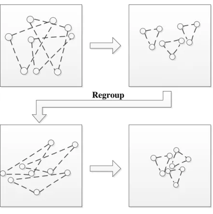
A. Small Sized Swarms
PSO needs a comparatively smaller population size, particularly to solve the simple problems, as a population with four to six particles can achieve best results. Conversely, the other evolutionary algorithms prefer larger populations, while smaller neighbourhoods yield good results and perform better for complex problems. Hence, in the new version, small neighbourhoods are used. In order to slow down the population’s convergence velocity and increase diversity, the DMS-PSO, divides the population into small sized swarms, each of which uses its own members to search for better areas in the search space.
B. Randomly Regrouping Schedule
Swarms of small sizes are looking for the best use of their own historical data, which is easy to converge to a local optimum, as are the property of convergence of the PSOs. In this case, it can keep the same neighbourhood structures, there will be no exchange of information between the swarms, and PSO will co-evolve these swarms in parallel investigation. In order to prevent this, a program is imported into the random rearrangement. Each R generations the population is grouped randomly and searching beings with a new configuration of small swarms. This period is called the group R. Thus, good information will be obtained to be exchanged between each swarm, although the diversity of the population increases. The new neighbourhood structure has more freedom compared to the conventional neighbourhood structure, resulting in better performance for complex multimodal problems.
Regroup
Figure 2.4: DMS-PSOs search(J. Liang & Suganthan, 2005).
Figure 2.4 shows how to regrouping schedule whereby the swarm is divided into three new random swarms with three particles in each one. Subsequently, the three flocks of particles are searching for better solutions individually. During this period, they may converge to the closed a local optimum. Subsequent regrouping leads to redistribution of the population in new swarms, which start searching. This process continues until a stopping criterion is met. The program is scheduling all particles swarms to regroup in new configurations so that each small swarm’s search space is enlarged, increasing the chance of finding better solutions using new small swarms (S. Zhao, Liang, Suganthan, & Tasgetiren, 2008) . At the end of the search, in order to perform a better local search, all the simple particles from the each swarm become a GPSO version. The pseudo code of DMS-PSO is given in Figure 2.5.
Figure 2.5: DMS-PSO sequence.
2.4.5 DMS-PSO with Sub-regional Harmony Search (DMS –PSO- SHS)
The dynamic multi-swarm particle swarm optimiser (DMS-PSO) with sub-regional harmony search (SHS) cross-breeds to obtain DMS-PSO-SHS. A modified algorithm called multi-trajectory search (MTS) is widely applied in various selected solutions. Effectively, variety maintaining population diversity puts more dynamic properties of swarms in DMS-PSO. Without crossing operation in high operational characteristics, HS intersection operation converts multiple parents of overall search behaviour for the proposed DMS-PSO-SHS. The entire population of PSO is divided into several swarms, as population individuals into a large number of sub-swarms are often grouped into individual HS population. These sub-sub-swarms are regrouped regularly by various programs and information is exchanged between the particles in the whole swarm. Therefore, diverse existing multi-swarm PSOs or local-version PSOs emerge, and the sub-swarms are small but dynamic, which is useful for a population and is appropriate for harmony research. Moreover, the last selected solutions from external memory are used to improve the diversity swarm.
The equation of the original HS algorithm are specified as the harmony memory and stored on feasible vectors (Lee & Geem, 2005), (Omran & Mahdavi, 2008) as shown in equation 2.9.
m: Each swarm’s population size n: Swarms’ number R: Regrouping period
Max_gen: Max generations, stop criterion Initialize m×n particles (position and velocity) Divide the population into n swarms randomly,
with m particles in each swarm. For i=1:0.9×Max_gen
Update each swarm using local version PSO If mod(i, R)==0,
Regroup the swarms randomly, End
𝐻𝑀 = [ 𝑥11 𝑥 21 … 𝑥12 𝑥 22 … ⋮ ⋮ … 𝑥1𝐻𝑀𝑆 𝑥 2𝐻𝑀𝑆 … 𝑥𝐷1 𝑥𝐷2 ⋮ 𝑥𝐷𝐻𝑀𝑆 || 𝑓𝑖𝑡𝑛𝑒𝑠𝑠(𝑥1) 𝑓𝑖𝑡𝑛𝑒𝑠𝑠(𝑥2) ⋮ 𝑓𝑖𝑡𝑛𝑒𝑠𝑠(𝑥𝐻𝑀𝑆)] (2.9)
where HMS is harmony memory size, and the candidate set [ x1, x2, …, xHMS] are the
rules number with D is the number of parameters (Geem, 2009).
As explained previously, the DMS-PSO-SHS is the hybridization of DMS-PSO and the regional harmony search (HS), which is based on the current pbests in each sub-swarm after PSO positions are updated. Nearest pbest is replaced by better fitness from with new harmony. MTS modified algorithm implements new line search along the dimension one by one. In addition, a method for improving diversity is used to improve the diversity of the swarm with a relatively low frequency and for timely discourage convergence in the right steps during the early search stage. The DMS-PSO-SHS modification with MTS attempts to take advantage of the PSO, HS and MTS to sidestep all particles are found in the lower regions local optimum. DMS PSO-SHS makes the particles several examples teach after swarms are often grouped and have greater harmony research among different sub-populations potential space. The DMS-PSO-SHS rejects the parameters of original HS, which usually need to be adjusted based on the property of the test problems, such as the bandwidth.
2.4.6 Adaptive Particle Swarm Optimisation (APSO)
Adaptive particle swarm optimiser (APSO) provides a better search performance and more efficiency than basic PSO. More importantly, it enables the performance of a global search space at a speed of convergence. The APSO consists of two phases: first, by examining population distribution and particle fitness, a method for the estimation of the evolution status in real-time is carried out on the four stages of identity evolution defined below, including the exploration, exploitation, convergence and jumping out in each generation. Also, its enables the automatic control of inertia weight, acceleration coefficients and other performance parameters to improve search algorithms, efficiency and speed of convergence. Then, it makes a statement of changes elite learning strategy when the state is classified as convergence. The strategy will focus on globally best particle to jump out of the likely local optima (Zhan, Zhang, Li, & Chung, 2009).
A. Population Distribution Information
The most prominent step that has been focused by APSO is based on complex analysis procedures on the population itself. In this section, PSO process and studied the characteristics of the population distribution for the first time to make an evolutionary state estimation approach. The distribution of information can be formulated as shown in Figure 2.6.
p2 p1 p3 g p4 p5 p2 p1 p3 g p4 p5 p2 p1 p3 g p4 p5 (a) (b) (c)
Figure 2.6: APSO population distribution information quantified by evolutionary factor f. (Zhan et al., 2009).
By calculation of the average particle distance of each of the other particles, it is reasonable to expect that the average distance between the global best particles with other particles in the state of convergence would be minimal as shown in the Figure 2.6 (a) the distance dg ≈ dpi during exploration, Figure 2.6 (b) the distance dg
dpi during exploiting and Figure 2.6 (c) the distance dg dpi during the jumping
out whereby the gbest is inclined to be surrounded by the swarm. In contrast, the average distance would be the maximum distance when jumping out of the state, because the global best is likely to be crowded away from the swarm. Therefore, evolutionary state estimation focuses on the dissemination of information to the population in each generation, as in the following steps:
Step 1: calculate the average distance of each particle i for all the other particles. This can be measured using the Euclidian metric equation:
𝑑𝑖 = 1 𝑁 − 1 ∑ √∑(𝑥𝑖𝑘− 𝑥𝑗𝑘) 2 𝐷 𝑘=1 𝑁 𝑗=1,