Impact of Stock Recommendations on Finnish Stock Market

(1)

THE SCHOOL OF ACCOUNTING AND FINANCE

Iiro Luomala

Impact of Stock Recommendations on Finnish Stock Market

Master Thesis Finance

(2)

(3)

UNIVERSITY OF VAASA

School of Accounting and Finance

Author: Iiro Luomala

Topic of the thesis: Impact of stock recommendations on Finnish Stock Market

Degree: Master of Science in Economics and Business

Administration

Master’s Programme: Finance

Supervisor: Timo Rothovius

Year of entering the University: 2014

Year of completing the thesis: 2019 Number of pages: 70

ABSTRACT:

Stock recommendations have gain interest, and became more important over the past years. Thus, brokerage houses are spending more and more money to examine companies and then, investors are following those recommendations. Hence, the purpose of the thesis is to exam-ine whether stock recommendations may generate positive abnormal returns. Earnings gen-erated by stock analysts’ recommendations can be considered to be an anomaly, that is, a deviation from the efficient market hypothesis. According to Fama’s (1970) efficient market hypothesis, all information should be available and new information should reflect to prices immediately when the new announcement is given.

Stock recommendations can be divided into five groups based on stock analysts’ recommen-dations; strong buy, buy, hold, sell and strong sell recommendations. Based on analysts’ con-sensus recommendations, five portfolios are formed, whose performance is under investiga-tion. When a company is given a recommendation, it is added to a specific portfolio and the company’s return is calculated. When the consensus recommendation changes, the company will be moved to another portfolio and the return will be recalculated. The thesis studies stock prices and returns of 62 companies from the Finnish stock market between 2010 and 2018. The hypothesis of the thesis is tested by several statistical methods, such as an ordinary least square and panel data methods. The results of both statistical methods are corresponding, thus strong buy, buy and unexpectedly, also strong sell recommendations, generate positive abnormal returns while sell recommendations produce negative abnormal returns during the observation period. Neither panel data methods nor OLS regression could find any statisti-cally significant results for hold recommendations.

(10)

(11)

1. INTRODUCTION

The stock recommendations of research analysts are interesting to investors, companies and academic researchers because brokerage houses are using millions of dollars to investigate companies and their analysts’ statements and opinions are published in magazines, newspa-pers and on television as well. However, Lin & McNichols’ (1998) results show that the impact or strength of recommendation depends on the independence of analysts, as all ana-lysts are not independent and external factors can influence on the recommendations. It is important to investigate the impact of recommendations thus market participants such as traders, companies, banks and institutions are investing money on the stock markets based on those recommendations which may not have completely independent.

According to Fama’s (1970) the Efficient Market Hypothesis (EMH), stocks should consist of all the information that is available and this should reflect rapidly to the stock prices. Based on this assumption, the stock analyst should not be able to produce any information that would change stock prices to one way or another. In that case, there should not be a possibility to achieve abnormal returns by following the stock analyst’s recommendations.

During the observation period, there has been ups and downs. For example, in 2011, the stock market faced the financial crisis, and because of that stock prices decreased strongly. Since 2012, prices have been increased almost without any exceptions and that can be seen from Figure 1 that represents OMXH Price Index’s development. OMXH PI-index will be used as a benchmark index in this thesis.

(12)

Figure 1. Development of OMXH PI-index

1.1. Purpose of the study

The motivation of this study is to examine whether there are any profitable ways of using stock recommendations to achieve positive abnormal returns. That will be tested by ordinary least square regression analysis and additionally, the statistical significance is also investi-gated by panel data methods, which provide some robustness check whether the effect of recommendations have any impact on stock returns. There is also used a modified panel data model which take into account lagged returns and it allows to examine whether the returns are auto correlated or is the effect due to a recommendation.

This thesis includes a daily stock recommendation, prices and returns from the Helsinki Stock Exchange from January 2010 to the end of October 2018. There are 62 companies whose recommendations have been taking into account and based on these recommendations, port-folios are formed. Then, the returns of each portfolio are calculated and then their statistical

0 2000 4000 6000 8000 10000 12000 1.1.10 1.1.11 1.1.12 1.1.13 1.1.14 1.1.15 1.1.16 1.1.17 1.1.18

(13)

significance is tested by different methods. Companies are in the specific portfolio that time while the specific consensus recommendation is on, and then, when the consensus recom-mendation changes, the company will be moved to another portfolio and returns will be re-calculated.

It is interesting to see whether the recommendations have any impact on stock prices and is there any possibility to achieve positive abnormal returns by following recommendations in Finnish stock market and break the assumptions of the efficient market hypothesis. If there is not any significant evidence of stock recommendation’s impact on stock returns, then in-vestors may consider whether there is any sense to follow and invest based on those stock recommendations. Stickel (1995) find an evidence that sell and buy recommendations have a stronger impact on stock returns comparing to hold recommendations in the U.S stock mar-ket. Also, Stickel’s (1995) results show that the effect of the recommendation is depended on a few different factors such as a reputation of analyst and size of brokerage-house. Based on those findings, there may be presented an assumption that also some statistically signifi-cant effects would be found in Finnish stock market.

1.2. Hypothesis

This study consists of one hypothesis that is shown below. The hypothesis supposes that there is no possibility to achieve positive abnormal returns by following stock recommendations by analysts. The hypothesis will be tested by several statistical methods and if there can find any statistically significant result of abnormal returns, then the null hypothesismust be re-jected.

H0: Portfolios based on recommendations cannot generate positive abnormal returns

(14)

1.3. Structure of the thesis

The structure of this thesis is the following: after introduction, there will be the theoretical part that contains the efficient market theory, the anomalies and the behavioural biases. This part gives a robust scientific basis for the thesis. The third chapter concentrates on different valuation models and it offers a solid background to the theory of the valuation modelling. There will be introduced models such as the CAPM, the Free Cash Flow, the Dividend Dis-count Model, the Gordon’s model and the Arbitrage Pricing Theory.

The fourth chapter introduces the analyst’s role in stock markets and there will be explained how analysts behave in the stock markets and what is their purpose to give recommendations. There will be introduced earlier research results of stock recommendations’ impact on the stock market. Also some strategies that based on stock recommendations will be presented. The fifth chapter represents data and methodology part in which there will be presented all the relevant data and the methods of how the thesis has been done. There will be shown the methods to examine abnormal returns and also the methods of different panel data models. In the sixth chapter, there is the empirical part in which contains results of the performance of the portfolios, the results of ordinary least square and panel regressions. In the end, there will be the seventh chapter that covers the conclusion of the thesis.

(15)

2. LITERATURE REVIEW

2.1. Efficient Markets

The efficient market hypothesis has been the central propositions since 1970 when Eugene Fama represents that the EMH consider how information reflect the security prices. Theoret-ically, neither fundamental nor technical analysis can produce excess returns. The efficient market hypothesis can be dived into three factors that are weak-form tests, semi-strong-form tests and strong-form tests. First, weak-form tests, in which the prices are affected by histor-ical information. Second, semi-strong-form tests, in which publicly available information may have an impact on the prices. Then, strong-form tests, in which all the information are already in the prices including inside information. (Shleifer 2000.) All the mentioned forms are described below in Figure 2. The figure shows that strong-form contains both, semi-strong-form and weak-form, thus semi-semi-strong-form count in weak-form and then weak-form describes only past information.

Strong-form

Semi-strong form

Weak-form

(16)

According to Fama (1970), the EMH can be summarized as follows; the markets are con-cerned about whether the prices are “fully reflect” available information at any point in time. While investors are acting rationally, they value the security for its fundamental value; the net present value of its future cash flows, discounted by the risk factors. When investors learn something about those securities’ fundamental values, they respond fast to the new infor-mation by bidding them down if the news is bad and bidding up if the news is good. Because of that, security prices include all the information that is available almost immediately and the prices rectify to new levels that are equivalent with the new net present values of cash flows. (Shleifer 2000.)

Shleifer (2000) adds that the EMH does not die or live by investors’ rationality because in many scenarios markets are still predicted to be efficient, even some investors are not acting rationally. It is said that the irrational investors are trading randomly in the market. When there is a lot that kind of traders, and when their trading strategies are uncorrelated, their trades are likely to cancel each other out. In that case, there will be significant trading volume as the irrational investors are trading securities with each other, but the prices are not close to their fundamental values. The EMH can be made even in the situations where the trading strategies are correlated.

An important effect of efficient market theory is that stock prices should follow a random walk. The term random walk represents the future movements of the variable that cannot be predicted because the variable is just as likely to rise as to fall. (Mishkin 1994.) According to Malkiel (2015), changes in stock prices are unpredictable and they are following a random walk. In the markets, there are a lot of players whose are selling their services but in the case of the EMH, investment forecasts and advisory services are worthless because of people are spreading information that affects the prices and all the secrets are already out to everyone. Randomly developing stock prices might be the necessary outcome of intelligent investors competing to observe relevant information on which to sell or buy a stock before the other of the market becomes aware that information (Bodie et al. 2014: 350).

(17)

as overreaction is. In earlier studies, such as in the EMH, is said that the prices overreact to information. Markets are consistently market efficient while anomalies are divided randomly between overreaction and underreaction. Fama proposes that an even split between underre-action and overreunderre-action is a good description of the existing anomalies. Even though, the most long-term return anomalies might be disappearing because of the changes in analysing techniques. Patell & Wolfson (1984) represent that most of the stock prices response to cor-porate earnings or dividends notifications appear within 10 minutes of the notifications.

2.2. Anomalies

Technical analysis has a narrower range of information to create portfolio than does funda-mental analysis. Investigations of the efficiency of fundafunda-mental analysis ask if publicly avail-able information beyond the trading history of an asset can be used to enhance investment performance. Findings show that it is difficult to recognize the efficient market hypothesis and therefore it is often referred to as efficient market anomalies. An anomaly describes an event where actual earnings differ from expected results that based on models. (Bodie et al. 2014: 366.)

There are several good examples of anomalies. Rolf Banz (1981) represents that firm size has an impact on a portfolio’s returns. Average annual returns are systematically higher on the small-firm portfolios. It is good to remember that smaller-firm portfolios bear more risk than higher ones. On the other hand, when returns are adjusted for risk by the CAPM, there is a coherent premium still for the smaller-sized portfolios. A few years later, researchers (Blume & Stambaugh 1983; Keim 1983; Reinganum 1983) proved that the small-size effect is the strongest in the first two weeks of January. The effect is called a January effect. The P/E-ratio anomaly stands that stocks with extraordinarily low P/E-ratios earn larger risk-adjusted returns than stocks with high P/E-ratio. It is said that this anomaly based on mis-specification of the CAPM. The P/E-ratio is said to be a proxy for some miss out factor hence that factor would include in the model, it would remove the anomaly. (Basu 1977; De Bondt

(18)

& Thaler 1985.)

Jegadeesh & Titman (1993) were the first researchers who proved that it is possible to create statistically significant abnormal returns using the Momentum-strategy. The research based on Rober Levy’s (1967) relative strength theory in which investors buy stocks that are in-creasing and sell stocks that are dein-creasing.

According to the EMH, new information should affect stock prices rapidly, for example, the stock prices should jump immediately after good news. But there is also an anomaly and it is called the Post-Earnings-Announcement Price Drift. (Bodie et al. 2014: 369.) Ball and Brown (1968) published an article in which after the company’s announcement the cumula-tive abnormal returns continue to increase (decrease) after good (bad) news. In that case, stock prices do not respond to new information immediately.

2.3. Behavioural Biases

Many research summarizes that investors are not able to do fully rational decisions even the information processes were perfect. These behavioural biases mostly affect how people are

framing questions of return versus risk, and in that case, make risk-return trade-offs. Inves-tors’ decisions seem to be affected by how choices are framed. For example, an individual investor may refuse a bet when it is caused in terms of the risk surrounding possible gains but may accept the same bet if described in terms of the risk surrounding potential losses. (Bodie et al. 2014: 391.)

One well recognized behavioural bias is overconfidence. Investors tend to overestimate their skills, abilities or knowledge. It has been noticed that people rank themselves better than other human beings, it is called as a better-than-average effect. Overconfidence may lead investors to make poor investment decisions on stock markets. (Bodie et al. 2014: 390.) Coval & Shumway (2005) research concludes that trader’s loss aversion has an impact on prices and a trader who lost money in the morning is 15% more likely to make such a trade

(19)

also in the afternoon than an investor who earned money in the morning. There are significant results of price changes done by loss-averse traders thus a trader that has lost money in the morning takes additional risk 27% more than if he gained profit in the morning. They con-cluded that there is more afternoon risk following morning losses than following morning profits.

Another behavioural bias is the Regret Avoidance. Psychologists have found that people whose decisions turn out badly, blame themselves more when that decision was more uncon-ventional. For example, buying Apples’ stocks that turn down is not as painful as having the same losses on an unknown start-up company. This decision is easier to attach to bad luck rather than bad decision making and bring less regret as well. (Bodie et al. 2014: 392.)

2.3. Limits to Arbitrage

The theory of limited arbitrage based on the behaviour of rational investors, called arbitra-geurs, thus economics is better at understanding and modelling that kind of behaviour. Be-havioural biases would not matter for stock pricing if arbitrageurs would fully use the mis-takes of investors. Behavioural supporters argue that there are a few factors that limit the ability to create profit from mispricing. (Shleifer 2000; Bodie et al. 2011: 414.)

According to Sheleifer & Vishny (1997) the model suggests where anomalies are probably to occur in financial markets, and why arbitrage fails to eliminate them. They show that per-formance-based arbitrage cannot fully be effective in bringing asset prices to fundamental values. Professional arbitrageurs may evade highly volatile arbitrage positions because of the risk of losses even though average return may be attractive. The idea of the efficient markets based on the supposition that most investors see and then take the available arbitrage possi-bilities such as the small firm anomaly. In fact, arbitrage resources are strongly concentrated only on a few investors who are specialized in that. After all, there are a relatively small number of investors understand the return anomaly well enough to exploit it.

(20)

3. VALUATION MODELS

3.1. Capital Asset Pricing Model

The capital asset pricing model (CAPM) is one of the most common known pricing models for securities and it is considered as a centrepiece of modern financial economics. The CAPM was published by three researchers, William Sharpe (1964), John Litner (1965) and Jan Mos-sin (1966). Those articles were a continuation of Harry Markowitz modern portfolio theory that was published in 1952. (Bodie, Kane, Marcus 2011: 308-345)

The CAPM provides a benchmark rate of return for estimating possible investments. It also offers an opportunity to make an educated suppose to the expected return on securities that have not been traded in the marketplace. The formula of CAPM is written as below (Bodie, Kane, Marcus 2014: 291-323.):

(1) E(Ri) = Rf + iE(Rm)  Rf

where E(Ri) = Expected return of portfolio i

Rf = Risk - free rate i = Beta of the security

E(Rm) = Expected return of markets

While using the capital asset pricing model, there have to use some simplifying assumptions. These assumptions ignore many real-world complexities but on the other hand, it gives us

(21)

some robust insights into the nature of equilibrium in security markets. (Bodie et al. 2011: 308-345)

1. There are many investors with small income comparing to the total in-come of all investors. There is the perfect competition assumption, thus investors are price-takers whose trades do not have an impact on the prices.

2. All investors have the same time horizon and holding period.

3. Investments are only publicly traded financial assets, such as bonds and stocks. Investors can lend or borrow at a fixed risk-free rate.

4. There are no taxes or transaction costs.

5. All investors are rational mean-variance optimizers.

6. All investors analyse assets in the same way and they have similar ex-pectations as well.

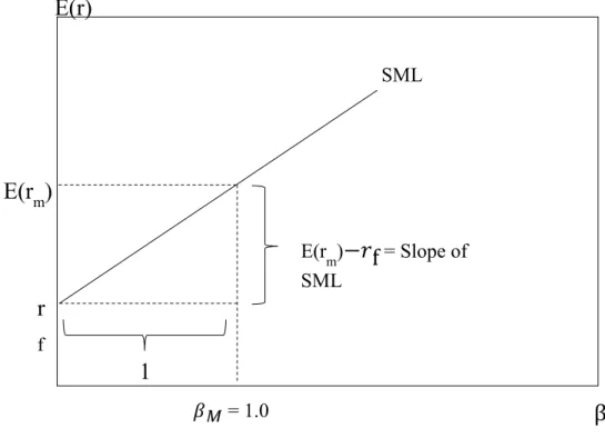
The expected return-beta relationship can be described graphically, as the security market line (SML) in Figure 3, which is as well a visual representation of the capital asset pricing model, where the y-axis of the chart represents expected return and x-axis of the chart repre-sents beta (market risk). When the risk and expected return are in relation to each other, then fairly priced securities lie on the SML. All assets have to lie on the SML in the market equi-librium. (Bodie et al. 2014: 291-323.)

(22)

The CAPM suppose that all investors are optimizing their portfolios according to Markowitz (1952) portfolio theory. All individual investors should use an input list to draw an efficient borderline using all available risky assets and recognize an efficient risky portfolio, P, by drawing the line CAL (capital allocation line) to the borderline, as in Figure 4. As a conse-quence, all the investors hold assets with weights appeared by the Markowitz optimization process. Because the market portfolio is the aggregation of all the identical risky portfolios, it also will have the same weights. In this case, if all investors choose the same portfolio with the same weights, it has to be a market portfolio. Therefore, the CAL based on individual investor’s optimal risky portfolio and in fact also, it will be the capital market line CML) that is represented in Figure 5. This suggestion let us say much about the risk-return ade-off. (Bodie et al. 2014: 291-323.)

SML

𝛽𝑀 = 1.0

E(r

_m

)

E(r)

Figure 3. The security market line (Bodie et al. 2014: 298.)

β

1

E(r_m)

−𝑟f

= Slope of SML

r

f

(23)

CAL (P) Efficient Frontier P ℴ𝑝 E(r_p) E(r) ℴ Figure 4. The Efficient Frontier of Risky Assets with the Optimal CAL (Bodie et al. 2014: 292.) CML Efficient Frontier M ℴM E(r_m) E(r) ℴ Figure 5. The Efficient Frontier and the Capital Market Line

(24)

3.2. The Arbitrage pricing theory

An arbitrage is an opportunity in which investor may earn profits without any risk. Four example, to buy an asset X on the New York’s stock exchange and then selling the same instrument X at the higher price on the London stock exchange. That situation would not be possible in case of if markets would be effective. That chance of arbitrage disappears rapidly because each investor wants to take an as large position as possible, thus investors bring back the equilibrium of the price. The equilibrium is also known as the Law of One Price, which states if two securities are equivalent in all economic aspects, then they should have the same market price as well. (Bodie et al. 2011: 351-354; Brealey & Myers 1991: 169-170.)

Stephen Ross (1976) was the first who introduced the arbitrage pricing theory (APT) and like CAPM, the APT links expected returns to risk and forecasts a security market line. The APT provides three key assumptions: first, assets yield can be presented by a factor model. Sec-ond, there are enough securities on the market to diversify away unsystematic risk. Third, well-functioning security markets do not permit the stability of arbitrage opportunities. The APT does not determine what those factors are, there could be a currency factor, an interest rate factors or even an oil price factor. The APT states that the expected risk premium on a share depends on the expected risk premium associated with each factor as well as the stock’s sensibility to each factor. (Bodie et al. 2011: 351-354; Brealey & Myers 1991: 169-170.) The APT can be shown as:

(2) Ri =  + b1(rfactor 1) + b2(rfactor 2) + … + ej

Where,

(25)

 = Is a constant for the asset

b1 = Expected risk premium associated with the sensitivity of

factor 1

b2 = Expected risk premium associated with the sensitivity of

factor 2

ej = Asset’s idiosyncratic risk

The APT stands that estimated expected returns depend on evaluated factors and variables such as the standard deviation, (highly correlated with estimated expected returns), do not add any extra explanatory capability to that of the factor loadings (Roll & Ross 1980).

3.3. The Fama-French (FF) Five-Factor Model

Eugene Fama and Kenneth French (2015) represents the Three-Factor Model in 1993, which have come to lead empirical model to analyse stock returns. The Three-Factor Model analyse the relation between size and average return and the relation between average price ratios such as B/M and average returns.

In 2015, Fama & French added two other factors (profitability and investment) to the model and now it is known as the Five-Factor Model. The model can be presented as follows:

(3) Rit = i + RMt+ SMBt + HMLt +RMW + CMA + eit

(26)

portfolios minus the return of large stock portfolios.

HML = High Minus Low, (value factor) thus the return of stock portfolios with a high book-to-market ratio minus the return of a stock portfolio with a low book-to-market ratio.

RMW = Robust Minus Weak, (profitability factor) is the difference of diversified portfolio’s stock returns with robust and weak profitability

CMA = Conservative Minus Aggressive, (investment factor), is the difference of diversified portfolio’s returns with high and low investment companies

Fama and French have chosen factors SMB and HML because of long-standing observations that corporate funding (company size) and book-to-market ratio forecast deflection of aver-age stock returns that corresponding with the CAMP. The model’s empirical grounds have been justified by Fama and French: HML and SMB are not themselves significant candidates for essential risk factors because of those variables might proxy for unknown fundamental variables. Fama and French represent that companies with high book-to-market ratios are more likely to be in financial suffering and small stocks might be more sensitive to changes in business circumstances. In this case, the variables may take sensitivity to risk factors in the macro economy. (Bodie et al. 2014: 340-341.)

When Fama & French added profitability and investment factors to the model, they noticed that the value factor (HML) came redundant for describing the average returns. They also find an evidence that the portfolios with small stocks with negative exposures to CMA and RMW are the biggest asset pricing problems in their empirical tests. (Fama & French 2015.)

(27)

3.4. Dividend Discount Model

John B. Williams introduced the Dividend Discount Model (DDM) in 1936 and now it is one of the most used valuation models. The DDM describes how the value of the company is determined using future dividends. Thus, the intrinsic value of the stock is the present value of the dividend that will be earned at the end of the first year. Future values and dividends are unknown hence variables will be only estimated. On the other hand, dividends can be hard to forecast for a longer period, thus something other such as cash or earnings should be predicted instead of dividends. Even slightly deviation of the forecast has a significant impact on the stock price thus the prediction used by the DDM must be as accurate as possible. If there are no expected dividend payoffs, then the model assumes that the stock has no value at all. To use the DDM correctly, it must be assumed that investors are expecting some pay-ments in the future. The model is seen a kind of umbrella model over the other discount models and those models are compared in terms of their formulas for the terminal value for the DDM. (Bodie et al. 2014: 591-596; Penman 1998.)

The basic formula of DDM is written as:

(4) 𝑉0 = D1 1+𝑘 + D2 (1+𝑘)2 + D3 (1+𝑘)3 + … + Dt (1+𝑘)𝑡

where, V0 = Current share price

Dt = Dividend payments at time t

(28)

3.5. The Constant-Growth Model

Using the DDM without any growth predictions is not pleasing because it demands dividend forecast for every single year into the inaccurate future. Myron J. Gordon (1956) introduced the Dividend Discount Model with growth assumption and it is better known as the Constant-Growth DDM or the Gordon’s Model.

The Gordon’s Model is derived from the basic formula of DDM and growth assumption has been added to it:

(5) 𝑉0 = 𝐷1

𝑘−𝑔

where, g = is a growth rate of dividends

The Gordon’s Model is universally used thus there are some limitations and implications. The model is only valid when g (growth rate) is smaller than k (rate of return) otherwise the value of the stock cannot be calculated. Also, a share value will be greater if its expected dividend is larger and if its expected growth rate is higher. (Bodie et al. 2014: 591-598.)

3.6. Free cash flow

An alternative approach to the DDM values is to use a company’s free cash flow (FCF). The free cash flow is available to the firm and its shareholders net of capital expenditures. This model is useful if the company does not pay dividends at all, so using the DDM is not rea-sonable. (Bodie et al. 2014: 618.)

(29)

The FCF can be presented as follows:

(6) FCF = EBIT (1 - tc) + Depreciation – Capital expenditures – Increase in NWC

Where, EBIT = Earnings Before Interest and Taxes tc = The corporate tax rate

NWC = Net Working Capital

As the DDM, the FCF uses a terminal value to evade adding the present values of an infinite sum of cash flows. The terminal value can be the present value of a constant growth for eternity or it can be based on EBIT-multiple, earnings, book value or free cash flow. There is a universal rule that estimates of natural value depend on terminal value. (Bodie et al. 2014: 618.)

According to Modigliani and Miller (1958), FCF and DDM should provide the same estimate intrinsic value if it is possible to determine a time period in which the company start to pay dividends that grow constantly.

3.7. Discounted cash flow (DCF)

The discounted cash flow (DCF) is a valuation method to estimate the value of the company by expected total free cash flows and discounting them to the present value. Company’s value today is always equal with the future cash flows that are discounted at the discount rate. The model based on the idea of the time value of money, thus a dollar today is worth more than a dollar tomorrow. As mentioned above, calculating present value, an investor must discount

(30)

expected cash flows by the rate of return presented by an equivalent investment in the capital market. That rate is called the discount rate, hurdle rate or opportunity cost of capital. (Brealey, Myers & Allen 2012.)

The DCF model is written as:

(7) PV =  𝐶𝑡

(1+𝑟_𝑡)𝑡 where,

PV = Present Value Ct = Cash flow at time t

rt = Discount rate

t = Time

The DCF is used to calculate the internal rate of return, thus the Net Present Value (NPV) is zero. The internal rate of return is often used in finance because it is a very useful model to find reasonable investments but as other discount models, it can be a misleading measure-ment if the numbers are inaccurate. (Brealey & Myers 1991: 30-90.)

To determine NPV, we may use the model above and add initial cash flow, Co, to it

Now the model is written as below: (8) PV = 𝐶𝑜

𝐶_𝑡 (1+𝑟_𝑡)𝑡

(31)

4. ANALYSTS ROLE IN THE STOCK MARKET

Stock market analysts are providing a significant part of the stock analyses and it is utilized by the fund managers in the equity markets. The analyses based on internal and external data, thus it is important to recognize the quality of the information and exploit it to create robust analyses and forecasts. Brokerage-firms provide a lot of background information and the analysts’ goal is to create forecasts of which fund manager decide is it valuable or not. (Dimson & Marsh 1984.) The recommendations can be dived in five categories: strong buy (1), buy (2), hold (3), sell (4) and strong sell (5) (Stickel 1995).

4.1. Who are the analysts?

Utilizing information and creating analyses is expensive thus brokerage-houses are using millions of dollars per year convincing investors that specific share is under- or overvalued and more attractive than other stocks. Even though, the research based on company-specific information such as earnings announcements or annual reports, still, the analysing is more predictive and evaluative. (Womack 1996.)

The semi-strong form of the EMH points that traders should not be able to earn profits that based on publicly available information which also recommendations are. However, broker-age-firms are using large amounts of money to analyse companies because they themselves and their customers believe that they can earn abnormal returns. (Barber, Lehavy and True-man research 2001.)

Research analyst may have a good relationship with the firm management, thus they are providing analyses for investment banks that are serving institutional clients who provide a commission to their brokers. To achieve these targets, there may be incentives that drive the analyst to create analyses, although the analyses may be biased. Analysts forecasts seems to have a significant increasing impact on brokerage-company’s stock price and that may be the

(32)

reason why brokerage-companies are incentivising market researchers. For example, strong buy and buy have a significantly greater effect on the trading activity rather than other (strong sell, sell, hold) recommendations. In that case, the incentives may lead analysts to give more easily buy or strong buy recommendation. (Irvine 2004.) Womack (1996) research shows that traders should only pay to brokerage-houses if they are expecting that the benefit is greater than the cost of the analyses.

Womack (1996) also finds that an incorrect sell recommendation may be riskier for an ana-lyst’s reputation rather than an incorrect buy recommendation because sell recommendation is more visible and less desirable. Womack came to the conclusion that an analyst’s expected compensation should be higher if the costs of sell recommendation are riskier.

According to Lin & McNichols (1998), hold recommendations have a significant negative impact on traders when an analysis is done by an affiliated analyst rather than a hold recom-mendation from an independent analyst. A hold recomrecom-mendation is seemed to be a bad an-nouncement also from a company’s perspective, and a hold recommendation from an affili-ated analyst is indicaffili-ated to be an even worse announcement. Their research also stands that affiliated analysts are avoiding sell recommendations to sustain customer relations. They are also able to show that an independent analysts’ recommendations are less favourable than an affiliated analysts’ announcements. Even though, an affiliated analyst may be over positive, their analyses of earnings are not more favourable than those analyses done by an unaffiliated analyst.

Schipper (1991) and Francis & Philbrick (1993) notice that researchers who are focused es-pecially on accounting are using a lot of energy analysing and making the cash flow and earnings forecast. Even though, those analyses are secondary while the main goal is to create correct recommendations. Sell and buy recommendations are following forecasts of share values using all obtainable information and data of industry as well as firm-specific infor-mation. Analyses are offering a direct test of the capability of well-informed market partici-pants to perform better than the stock markets on average. (Womack 1996.)

(33)

4.2. Factors that are affecting price-reaction

According to Fama’s EMH, new information should reflect rapidly in a security’s price and it is said that the EMH is an exact description of price behaviour in the stock markets. The information hypothesis means that when a large piece of stock is sold in the market, the price is expected to fall and this decreasing is the expected value of the information contained in the stock trades. The adjustment should be a permanent and not a temporary change followed by abnormal returns in the future, as the price pressure hypothesis supposes. The price pres-sure effect leads to a temporary price adjustment in the stock prices which will revert over time. (Scholes 1972; Barber & Loeffler 1993.)

Womack (1996) found a robust evidence that analyst’s recommendations have a significant impact on stock prices, and that effect is not only at the immediate time of the recommenda-tion announcement but also in following weeks. Womack’s research concludes that sell rec-ommendation may harm a brokerage-house’s potential and present investment banking rela-tions and that may restrict access to information if an analyst gives unfavourable recommen-dations. Womack concludes three different empirical results; (i) The first reaction to changes in the recommendation appears to be permanent. Thus, the recommendations contain a sig-nificant information for which a brokerage-house must be compensated. (ii) The changes seem to be mostly unsolved problems and those findings can be categorized on underreaction and subsequent changes associated with an announcement events such as stock repurchases, earnings announcements or dividend initiations. (iii) Analysts’ new buy recommendations seem to appear seven times often than new sell recommendations thus analysts are not happy to give sell recommendations because the costs of giving sell recommendations are larger. Brokerage-companies’ sell and buy recommendations have a short-term price impact on share prices which consists of the six different components: the reputation of the analyst, the strength of the recommendation, the size of the brokerage-firm, the size of the recommended company, the change in recommendation and contemporaneous earnings forecast revision. (Stickel 1995.) Those components are described below.

(34)

According to Stickel (1995), the reputation of the analyst affects stock prices stronger if the reputation is better. Stickel (1992) found direct evidence of the positive relationship between performance, reputation and stock prices, thus analyst with great performance record and reputation may create greater impact rather than an analyst whose record is not that impres-sive. Sorescu & Subrahmanyam (2006) find that the abnormal returns are significantly neg-ative after large recommendation changes done by the stock analyst who is employed by less approved brokerage-house or who is inexperienced.

Stickel (1995) created a hypothesis that various recommendations have a different level of the strength. In that case, thestrength of recommendations depends on analyst’s signals, for example, a buy recommendation signal tells that the firm is undervalued in the stock markets and then strong buy recommendation tells that the firm is even more undervalued. Because of that the stock price should react stronger to strong buy signal rather buy signal.

The size of the brokerage-house causes a price-reaction in short-term andsell or buy recom-mendations from large brokerage-firm have a stronger influence to prices than a recommen-dation by a smaller brokerage-company. The reason for this is because larger companies have more sale personnel and they may create a higher price effect. (Stickel 1995.) Womack (1996) found that recommendations by the large well-known brokerage-house are mainly based on well-followed stocks.

The fourth hypothesis stands that the size of the recommended firm influence on prices, thus larger firms have smaller price reaction to sell or buy recommendations than smaller firms. That is because of smaller companies’ information and data is not processed as efficiently as larger companies have. (Stickel 1995.) According to Womack (1996), the market reaction associated with larger capitalization companies is smaller than the market reaction with smaller capitalization companies.

The change in recommendation hypothesis stands that skipping a rank have a great impact on the share prices. For example, a change in the recommendation from hold to strong buy has a stronger influence than a revision from hold to buy. (Stickel 1995.) Womack (1996)

(35)

found that the market reaction between new buy signals and new sell signals is a significantly asymmetric and also the new sell recommendation has a stronger influence on markets. The last hypothesis, contemporaneous earnings forecast revision have a greater impact on stock prices than recommendations that are done without a corresponding revision of the earnings forecast. (Stickel 1995.)

4.2.1. Dartboard research

The “Dartboard” column is a contest that is testing the efficient market hypothesis and it is published monthly in the Wall Street Journal. It contains a stock recommendation by four professional portfolio manager and strategist. Those stocks picked by experts are competing against the random selections of four general darts. Beginning of the month, four profession-als are selecting the one stock that they believe to generate mostly profit over six months and the stock must be traded on the NASDAQ, American or New York stock exchange. Eventu-ally after six months, those picks will be compared with the random selection of four darts. Some of the studies conclude that a price pressure effect has created abnormal returns but, on the other hand, some of the researchers have come to the conclusion that an information effect causes abnormal returns. (Barber & Loeffler 1993; Metcalf & Malkiel 1994.)

Metcalf & Malkiel (1994) did not find any evidence that the stocks chose by experts can outperform the markets systematically, even though the gross return data seem to assume that the expert’s picks reach excess returns. The professionals tend to choose riskier shares that are performing worse than the darts after controlling for risk. During the six-month compe-tition, the darts over-perform 15 times with 6.9% abnormal return meanwhile the profession-als beat the markets 18 times with 9.5% abnormal returns. Researchers conclude that if the market would be fully efficient, the probability of the darts’ or experts’ portfolios to win competition should be equal.

(36)

Barber & Loeffler (1993) find that stocks picked by professionals achieved over 4% abnor-mal returns for the two days after the announcement of the recommendation. They also notice that around half of this abnormal return revert during 25 trading days. Correspondingly, the Dartboard stocks did not achieve abnormal returns at all during the observation period. This research proves their hypothesis of the price pressure that some of the traders buy and sell securities based on experts’ recommendations which leads to a temporary price response in that particular stock. The fact that a part of the price reaction is sustainable the recommenda-tion may include some robust informarecommenda-tion. Albert Jr. and Smaby (1996) get similar results as Barber & Loeffler had a few years earlier. Assets picked by the expert in the Dartboard indi-cate meaningful positive return over the 50-day period following the two-day publication date reaction. However, Alber Jr’s and Smaby’s results differ from Barber’s and Loeffler’s results, as their research shows that the results are consistent with an information effect whereas Barber’s and Loeffler’s results are based on a price pressure effect.

Liang (1999) finds that there is a 2-day announcement effect after the analysts’ stock recom-mendation. During the first 15 days the announcement effect is reversed and actually that effect based on analysts’ past track record. Liang notices that if the analyst’s recommendation record in the past is great, then naive investors make their investment decisions based on that, even though the past is not a guarantee of the future. According to Liangs’ study, the price pressure hypothesis assumes that the analyst’s recommendation creates temporary buying pressure by naive traders and that buying pressure may create abnormal returns temporarily. On the other hand, the information effect predicts that analysts have inside information and their recommendations contain that inside information and then it creates temporary abnor-mal returns. Liang’s research concludes that there is an information leakage just before new recommendation hence both, abnormal returns and trading volumes, have a significant posi-tive effect for the analyst’s stock.

According to Ferraro’s and Stanley’s research (2000), either the Dartboard stocks or picked stocks by experts cannot create a significant abnormal return over time. But an analyst who earned abnormal returns in the previous competition is achieving significantly higher stock price performance than those who underperformed.

(37)

4.3. Strategies that based on recommendations

According to Barber et. al. (2001), it is possible to earn abnormal returns by following ana-lyst’s recommendations. Investors should buy stocks that are the most highly recommended and in contrast, investors should sell short stocks that are the least favourable recommended by analysts. Investors should daily rebalance their portfolios and follow the analyst’s con-sensus recommendations.

Barber et. al. (2001) findings show that buying shares that have a positive consensus recom-mendation with balanced daily portfolios along with right timely reactions to recommenda-tion may cause over 4% annual abnormal returns.

Barber et. al (2001) find that buying the shares with the highest consensus recommendation create almost 19% an annual return while buying the stocks with the least favourable con-sensus recommendation create approximately 6% annual profits. In contrast, a value weighted market portfolio outperformed 14.5 % annual return during the same period. Thus, a portfolio with the highest recommendation created over 4% abnormal returns and the less favourable portfolio’s abnormal return was almost -5% after controlling for factors such as market risk, price momentum and book-to-market effects. In addition, the best recommended shares outperformed the less favourable recommended stocks by 102 basis points per month. (Barber et. al. 2001)

Jegadeesh, Kim, Krische and Lee (2004) study shows that analysts prefer to give higher rec-ommendations to stocks that have high trading volume and positive earnings and price mo-mentum. Those shares tend to have higher sales growth and its earnings are expected to in-crease fast in the future. In addition, those shares may have greater valuation multiples as well. Researches find that recommendations are positively correlated with momentum strat-egy and recommendations are negatively correlated with contrarian investment stratstrat-egy. Thus analysts are preferring high momentum shares and growth stocks in their recommen-dations. Jegadeesh et. al. (2004) also find that the level of the recommendation is not that

(38)

robust as the power of the change is. Thus, there may have some relevant information con-tained with the analyst’s changes in the recommendation. In conclusion, an investor may earn abnormal returns by following the momentum strategy and following the change of recom-mendations.

(39)

5. DATA & METHODOLOGY

5.1 Data

This study’s data based on daily consensus stock recommendation from the Thomson Reuters database. The data contains all the stocks from Finnish exchange market (OMXH), stocks’ daily returns, OMXH PI-index and 3-month daily Euribor is used as a risk-free rate. The observation period is from January 2010 to the end of October 2018. This thesis manages stocks and recommendations only if a company have gotten recommendations for a whole observation period. Companies have been removed if they have been sold, they have not gotten any recommendations or they have been moved off from OMXH. After this screening, 62 companies met these terms. The consensus stock recommendations are the average of all the recommendations provided by analysts and the scale of recommendation is as formed as follows: 1 = Strong Buy, 2 = Buy, 3 = Hold, 4 = Sell and 5 = Strong Sell. The portfolios are constructed based on the mean of the recommendations. When a company is given a recom-mendation, it is added to one of the portfolios above, and the company’s return is calculated. When the consensus recommendation changes, the company will be moved to another port-folio and the return will be recalculated.

Also, there will be tested abnormal returns statistical significance by panel data methods. This part of the study consists of also daily consensus stock recommendations, but in this case, there have been constructed three portfolios instead of five; “Buy”, “Hold” and “Sell”. Strong Buy and Strong Sell consensus stock recommendations have been included in the “Buy” and the “Sell” portfolios. In that case, we can see what an impact is when extremity recommendations are included to more common recommendations.

(40)

5.2 Methods of the OLS regression

This part of the study focuses on to examine whether there is a possibility to achieve abnor-mal returns by following analysts’ stock recommendation in the Finnish stock market or not. There are five consensus portfolios that are updated if a company’s recommendation has been changed. Stocks’ daily returns are compared to OMXH-index’s returns in the same period. The first portfolio contains all the stocks that have gotten consensus recommendation “Strong Buy”, thus its average is 1 ≤ 𝑥it ≤ 1,5 at time t-1. The second portfolio contains stocks whose consensus recommendations are ”Buy” and its average is 1,5 < 𝑥it ≤ 2,5, the third portfolio is formed from stocks whose recommendations are “Hold” and the mean is 2,5 < 𝑥it ≤ 3,5. The fourth portfolio contains stock that has a consensus recommendation “Sell” and the av-erage is 3,5 < 𝑥it ≤ 4,5 and the last portfolio “Strong Sell” contains stocks whose consensus is 4,5 < 𝑥it ≤ 5. Then the consensus recommendation is calculated as a weighted average and the formula is shown below:

(9)

𝑥

_it= _𝑛1

𝑖𝑡

∑

𝑋𝑖𝑗𝑡

𝑛𝑖𝑡

𝑗=1

in which 𝑥it is the average of the recommendation for a company i at time t, nit is a number of the recommendations and Xijt is an individual recommendation for a company i at time t. The stock returns of each company are calculated by natural logarithm thus the results are then comparable. Daily returns of each company based on the cumulative returns of each individual stock returns’ average and the formula is shown below:

(10) R_it₌

∑

𝑛𝑡

𝑅

_𝑖𝑡

(41)

in which, Rit is a daily return of an individual stock i, Rit is a daily stock return at time t and nt is a number of trading days in a current month.

Portfolios returns are then calculated as a weighted average of individual stocks returns and the formula is as follow:

(11)

𝑃

it = 1

𝑛_𝑖𝑡

∑

𝑋𝑖𝑡 𝑛 𝑗=1

in which 𝑃it is the daily return of portfolio p, Xit is stock’s i daily return at time t and n is a number of stocks in the portfolio. The returns of portfolio Rpt are then compared to the mar-ket return Rmt (OMXH), thus the excess returns ARpt can be calculated. The formula is shown below:

(12) ARpt = Rpt - Rpt

The statistical significance of portfolios’ returns is examined by Jensen’s alpha and CAP-model. Portfolios’ returns and market returns reduced by risk-free rate (3 month Euribor) is placed in the equation (13) according to CAP-model and then the alpha of each portfolio can be calculated. The betas are calculated annually for each portfolio. The regression model is shown below:

(42)

where Rpt is the return of the portfolio, Rf is the risk-free rate,  is the intercept,  is the beta of the portfolio and Rmt is the market return.

Sharpe (1966) introduced a measure, reward-to-variability-ratio, also known as a Sharpe-ratio, for the portfolio’s performance. The Sharpe-ratio describes a portfolio’s risk-adjusted return and the better ratio is, the better is the portfolio’s risk-adjusted performance. If the Sharpe-ratio is negative, then the return is expected to be negative or the risk-free rate is higher than the portfolio’s total return. In that case, the Sharpe-ratio does not provide any valuable purpose. The formula of Sharpe-ratio can be written:

(14) Sharpe Ratio = 𝑅𝑝−𝑅𝑓 𝜎𝑝

Where, Rp = Return of portfolio

Rf = Risk-Free rate p = Standard deviation

Jack Treynor (1973) developed another risk measure for portfolios’ performance. It is known as the Treynor-ratio or the reward-to-volatility ratio that describes how much excess return was produced for each unit of market risk. The Treynor’s ratio is a sensitivity to changes in beta or market risk, thereby, diversification cannot eliminate that risk. The greater Treynor-ratio is better. The formula of Treynor-Treynor-ratio can be shown as below:

(15) Treynor Ratio = 𝑅𝑝−𝑅𝑓 𝛽

(43)

Where, Rp = Return of portfolio

Rf = Risk-Free rate  = Beta, market risk

5.3. Methods of panel data models

This part manages the methods of the second part of the thesis in which there will be exam-ined what is an impact of buy, hold and sell stock recommendations on stock prices and returns. More specific, there will be investigated what is an impact on stock returns when the recommendation changes from one to another. As mentioned before, there are three consen-sus portfolios that are “Buy”, “Hold” and “Sell” portfolios instead of five portfolios that were used in the OLS regression. Those portfolios are constructed by consensus stock recommen-dations and strong buy and strong sell recommenrecommen-dations are included to the “Buy” and the “Sell” portfolios. Stock returns are calculated in the same way that was in earlier part, thus the stock returns are calculated by natural logarithm therefore returns are comparable. This part of the thesis focus on the panel data methods thus the study’s data have both cross-sectional and time series elements. The panel of data will consist of an information across space and time and the panel maintain same objects and it measures them over time (Brooks 2008).

There is used the Hausman Test (also known as a specification test) to observe endogenous the predictor variables in a regression model. The Hausman Test examines whether the pre-dictor variables are endogenous or not and the model also sort out which model should be used in the analysis, the random effect model or the fixed effect model. If the assumptions of the random effect model do not hold, then the random effect model is less efficient than the fixed effect model. (Hausman 1978.)

(44)

There are three types of panel models that can be used to analyse this study’s portfolio’s data; the fixed effects model, the random effects model and the mixed likelihood model.

The fixed effect model is a statistical model in which intercepts are correlated with including variables. The model’s estimators are fixed unlike in the random effect model in which pa-rameters are random variables. Also a dummy variable can be added to the fixed effect model. (Brooks 2008.)

The fixed effect model can be shown as below:

(16)

y

it

=



+



x

it

+



it

+



it

,



it

=



i

+



it

where, yit is the dependent variable and  is the intercept term and the is a k x 1 vector of

parameters to be calculated on the explanatory variables. The term xit is a 1 x k vector of

findings on the explanatory variables. The itis an error term. It can be said that the term it

encapsulates all the variables that have an impact on the dependent variable yit and it does

not vary over time.The term itcaptures everything unexplained things that other variables

cannot explain about dependent variable yit. (Brooks 2008.)

The other model that is used is known as the random effect model which approach considers different intercept terms for each factor and those intercepts are constant over time and then, the relationship between the explained and explanatory variables supposed to be an equal both temporally and cross-sectionally. And the including variables are not correlated with the independent variables. (Brooks 2008.)

(45)

(17)

y

it

=



+



x

it

+



it

,



it

=



I

+



it

where, xit is a 1 x k vector of explanatory variables but there is no dummy variable as it was

in the fixed effect model. In the random effect model, the term I captures the heterogeneity

in the cross-sectional dimension. The  and  are same terms as they were in the equation X. (Brooks 2008.)

The maximum likelihood is a statistical method that is used to estimate all the possible equa-tions of the data thereby all the parameters that are selected are most likely to generate the observed data. The maximum likelihood method can find parameter values for both non-linear and non-linear models. Together with the maximum likelihood method, there is used a bootstrap simulation to reach a description of empirical estimators. (Brooks 2008.)

In each previously mentioned model, there is also used lagged method to estimate the impact of returns of the previous day on today’s stock prices in which the independent variable “re-turns” is lagged. It allows regarding results in different perspective.

(46)

6. EMPIRICAL PART

This chapter introduces the empirical part of the study. There are hypothesis that were pre-sented in the introduction and the hypothesis are shown below again. The hypothesis will be tested by several statistical methods to find out the statistical significance of the hypothesis and the results are shown in this chapter.

The hypotheses are written as follows:

H0: Portfolios based on recommendations cannot generate positive abnormal returns

H1: Portfolios based on recommendations can generate positive abnormal returns

6.1 Portfolios

The portfolios are constructed based on their consensus recommendation that was presented in the chapter “Data & Methodology”. This chapter presents each portfolio’s structure and measurement of performance such as Jensen’s alphas, Sharpe ratios, Treynor ratios, betas and standard deviations. Based on those metrics, portfolios can be compared and thereby seen which portfolios have performed best and which portfolios worst.

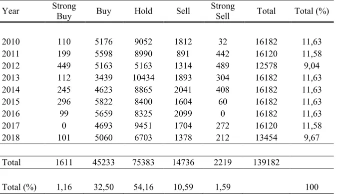
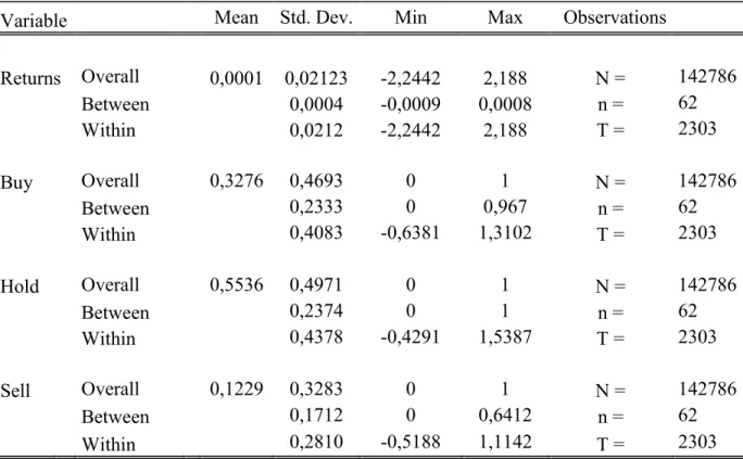
Table 1 contains numbers of the recommendations in each portfolio. As can be seen, the “Strong Buy” and the “Strong Sell” portfolio’s observations are the lowest ones thus analysts are not favourable to give extremity recommendations. The “Hold” portfolio contains most recommendations (75383), the “Buy” second most (45233) and the “Sell” portfolio got ap-proximately 15000 recommendations. About 54% of the recommendations are holds, 33% are buys, 11% are sells and then there is a small sample of recommendations for strong buy

(47)

and strong sell. This support assumption that analysts prefer to give a hold or buy recommen-dation than a sell recommenrecommen-dation.

Table 1. Number of the recommendations

Year Strong _Buy Buy Hold Sell Strong _Sell Total Total (%)

2010 110 5176 9052 1812 32 16182 11,63 2011 199 5598 8990 891 442 16120 11,58 2012 449 5163 5163 1314 489 12578 9,04 2013 112 3439 10434 1893 304 16182 11,63 2014 245 4623 8865 2041 408 16182 11,63 2015 296 5822 8400 1604 60 16182 11,63 2016 99 5659 8325 2099 0 16182 11,63 2017 0 4693 9451 1704 272 16120 11,58 2018 101 5060 6703 1378 212 13454 9,67 Total 1611 45233 75383 14736 2219 139182 Total (%) 1,16 32,50 54,16 10,59 1,59 100

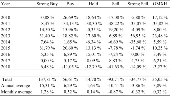
Table 2 represents portfolios’ and benchmark’s annual returns. As can be seen, the order of the portfolios is as expected thus the “Strong Buy” portfolio achieved highest returns mean-while the “Sell” and the “Strong Sell” portfolio performed worst.

(48)

Table 2. Annual returns of portfolios and market returns

Year Strong Buy Buy Hold Sell Strong Sell OMXH

2010 -0,88 % 26,69 % 18,64 % -17,08 % -5,80 % 17,12 % 2011 -8,47 % -34,13 % -38,30 % -48,22 % -35,07 % -35,82 % 2012 14,50 % 15,96 % -0,35 % 19,20 % -4,09 % 8,00 % 2013 31,40 % 18,82 % 17,60 % 6,89 % 56,95 % 23,48 % 2014 7,64 % 1,65 % -6,34 % -6,69 % -35,68 % 5,59 % 2015 81,79 % 26,60 % 13,13 % -7,78 % -1,74 % 10,25 % 2016 5,35 % 6,89 % 15,01 % -7,24 % 0,00 % 3,49 % 2017 0,00 % 5,17 % 8,09 % 8,83 % 4,75 % 6,21 % 2018 6,48 % -11,05 % -12,79 % -41,63 % -14,09 % -3,27 % Total 137,81 % 56,61 % 14,70 % -93,71 % -34,77 % 35,05 % Annual average 15,31 % 6,29 % 1,63 % -10,41 % -3,86 % 3,89 % Monthly average 1,28 % 0,52 % 0,14 % -0,87 % -0,32 % 0,32 %

The “Strong Buy” portfolio achieved the highest total returns (137,81%) and it has performed negative return only in one year when its return was -0,88%. Even though, the total perfor-mance of “Strong Buy” portfolio is the highest, still it was not the best portfolio in all the years. As can be seen, the “Strong Sell” was able to achieve higher returns in some years than the “Strong Buy” portfolio, even though, overall its returns are negative. The “Buy” portfolio’s total return is a positive (56,61%) and it has performed very well except years 2011 and 2018 when its total return was negative. It is interesting that the “Buy” portfolio achieved its the highest return in 2010, in the same year when the “Strong Buy” portfolio’s return was negative.

The “Hold” portfolio achieved positive total returns (14,70) and it was able to perform neg-atively only in four years. The “Sell” portfolio’s returns were negative (-93,71%) and actually its total performance is the worst comparing to other portfolios. The “Sell” portfolio reached a positive return only in 2012, 2013 and 2017. The “Strong Sell” portfolio’s total perfor-mance is negative while it achieved -34,77% total returns, even it has the highest return (56,95%) in 2013 when it beat all the other portfolios.

(49)

Only the “Strong Buy” and the “Buy” portfolios could beat the benchmark portfolio, OMXH which reached 35,05% total returns. The OMXH achieved positive returns in all years except in 2011 and 2018. None of the year its return was not the highest compared to other five portfolios.

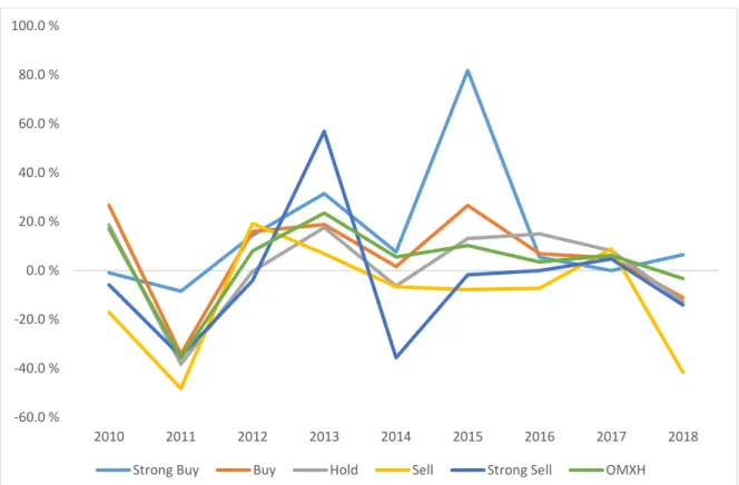
Figure 6. Annual returns of portfolios and OMX-index

Figure 6 shows market returns graphically, thus it can be seen that in some years all the portfolios performed poorly. For example, in 2011 none of the portfolios achieved positive returns. It may be due to the financial crisis that caused by Euro-zone problems. On the other hand, there are years such as 2013 and 2017 when all the portfolios achieved positive returns.

-60.0 % -40.0 % -20.0 % 0.0 % 20.0 % 40.0 % 60.0 % 80.0 % 100.0 % 2010 2011 2012 2013 2014 2015 2016 2017 2018

(50)

Table 3. Portfolios’ return reduced by a market return

Year Strong Buy Buy Hold Sell Strong Sell

2010 -18,01 % 9,57 % 1,52 % -34,20 % -22,92 % 2011 27,36 % 1,69 % -2,47 % -12,40 % 0,75 % 2012 6,49 % 7,96 % -8,35 % 11,20 % -12,10 % 2013 7,92 % -4,67 % -5,88 % -16,59 % 33,46 % 2014 2,05 % -3,93 % -11,93 % -12,27 % -41,27 % 2015 71,54 % 16,35 % 2,88 % -18,03 % -11,99 % 2016 1,86 % 3,40 % 11,52 % -10,73 % -3,49 % 2017 -6,21 % -1,03 % 1,89 % 2,63 % -1,45 % 2018 9,75 % -7,77 % -9,52 % -38,36 % -10,81 % Total 102,76 % 21,56 % -20,35 % -128,77 % -69,82 % Annual average 11,42 % 2,40 % -2,26 % -14,31 % -7,76 % Monthly average 0,95 % 0,20 % -0,19 % -1,19 % -0,65 %

Table 3 shows the return of portfolios reduced by a market return (OMXH). As we can see, only the “Strong Buy” portfolio and the “Buy” achieved positive total returns and outper-formed OMXH-index. The “Strong Buy” portfolio was not able to outperform OMXH-index in 2010 and 2017, thus in other years it beat the benchmark. Its total return is by far the highest. Also, the “Buy” portfolio has reached excess returns in five years and its total ab-normal returns are 21,56%.

Even though, the “Hold” portfolio’s market return was positive, it could not achieve excess returns comparing to the benchmark index OMXH. There are some years when the “Hold” portfolio’ achieved excess returns but as a whole its return is negative. The “Sell” portfolio’s performance is the worst and it was able to beat the OMXH only twice, in 2012 and 2017. The “Strong Sell” portfolio has outperformed as the OMXH in 2011 and 2013. In other years it could not achieve excess returns and its total returns were -69,82%.

(51)

Table 4. Portfolio’s measurements

Strong Buy Buy Hold Sell Strong Sell

Std. 0,27 0,19 0,19 0,22 0,27

Beta 0,17 0,65 1,10 0,57 0,04

Sharpe 0,55 0,31 0,07 -0,48 -0,15

Treynor ratio 0,89 0,07 0,01 -0,19 -1,09

As can be seen from Table 4, all the portfolios have a positive beta and the values are between 0,04 to 1,10. The “Hold” portfolio’s beta value is near one thus that portfolio is following the market best. The “Buy” and the “Sell” portfolios have almost same betas thus those portfolios follow market reaction same way. The “Strong Buy” and the “Strong Sell” have the lowest betas thus those portfolios react least to the market changes.

Comparing standard deviations, it can be seen that the “Hold” portfolio has the lowest vola-tility (18,60%) and the “Strong Buy” portfolio and the “Strong Sell” portfolio have the high-est volatilities. Other portfolios’ standard deviations are around 20%.

Sharpe ratios are as expected based on portfolios performance, thus the “Strong Portfolio” has the best ratio (0,55) and the “Sell” portfolio’s Sharpe is the lowest one. Also, the “Buy” and the “Hold” portfolios reached positive Sharpe ratios. Treynor Ratios are also following very well portfolios’ performance, thereby the “Strong Buy” portfolio, the “Buy” portfolio and the “Sell” portfolio reached positive ratios and the “Sell” and the “Strong Sell” portfolios reward-to-volatility ratio as a negative, as was the Sharpe ratios.

6.2. Results of the OLS regression analysis

The regression analysis measures if the results of abnormal results are statistically significant or not for the period from January 2010 to October 2018. The regression analysis is done by the simple linear regression model, Ordinary Least Squares (OLS). Each portfolio’s returns are calculated and after that returns are regressed by using the market-model to find out the

(52)

statistical significance of the Jensen’s alpha. The results of the regression analysis are pre-sented in table 5.

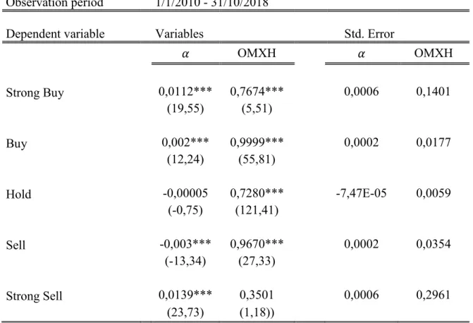
Table 5. The results of the Ordinary Least Squares Method: Ordinary Least

Squares

Observation period 1/1/2010 - 31/10/2018 Dependent variable Variables Std. Error

𝛼 OMXH 𝛼 OMXH Strong Buy _0,0112*** 0,7674*** 0,0006 0,1401 (19,55) (5,51) Buy _0,002*** 0,9999*** 0,0002 0,0177 (12,24) (55,81) Hold -0,00005 0,7280*** -7,47E-05 0,0059 (-0,75) (121,41) Sell _-0,003*** 0,9670*** 0,0002 0,0354 (-13,34) (27,33) Strong Sell _0,0139*** 0,3501 0,0006 0,2961 (23,73) (1,18))

* indicates statistical significance at the 10% level ** indicates statistical significance at the 5% level *** indicates statistical significance at the 1% level

As mentioned above, the regression is done by the OLS method, and there is one dependent variable (portfolio) and two other estimators which are 𝛼 and OMXH. The term 𝛼 describes Jensen’s alpha and OMXH is the benchmark portfolio reduced by risk-free rate.

(53)

As can be seen from table 5, the “Strong Buy” portfolio’s alpha is a significant at 1% level, thus it can be said that the results of the “Strong Buy” portfolio are highly significant. The “Strong Buy” portfolio’s alpha is a positive (0,0112) thus by following that portfolio, inves-tors may achieve abnormal returns. The results of the “Strong Buy” portfolio are expected because stock analysts are not giving the highest recommendations unless they believe that a company can perform exceptionally well. When stock analysts give a strong buy recom-mendation, they estimate that recommended company is even more undervalued and then investors start to buy shares of recommended company and its price increases to the right level.

The “Buy” portfolio’s alpha is a slightly positive (0,002) at a 1% significance level, whereby the results of the Jensen’s alpha are highly significant and investors may reach abnormal returns by following this