Classification centric Lloyd-Max quantizer for predictive feature errors

CLASSIFICATION CENTRIC LLOYD-MAX QUANTIZER FOR PREDICTIVE FEATURE ERRORS

BY

COREY SNYDER

THESIS

Submitted in partial fulfillment of the requirements

for the degree of Bachelor of Science in Electrical and Computer Engineering in the Undergraduate College of the

University of Illinois at Urbana-Champaign, 2018

Urbana, Illinois Adviser:

ABSTRACT

Conventional forms of image and video compression have a singular objective to optimize visual image quality in the presence of a target compression ratio. However, if we would like to perform machine analysis of these compressed images, what we as humans view as interpretable is distinct from what ma-chines may find informative. This paper will discuss compression techniques with the dual purpose of maintaining image quality and preserving image features for machine classification.

The format of our system is a two-part predictive encoder. Features are extracted from both the original and JPEG 2000 compressed images. The difference between these feature vectors are the resulting error vectors due to compression. We seek to build an efficient quantizer to encode the predictive feature errors. We evaluate the effectiveness of our quantizer by examining its ability to recover accuracy lost in an image classifier due to compression. We present the Classification Centric Lloyd-Max Quantizer as an efficient vector quantizer to restore feature vector integrity and maintain high com-pression ratios. We compare previous work that utilizes scalar Lloyd-Max Quantizers and gradient descent methods to build an optimal vector quan-tizer against our proposed system. We demonstrate the advantages and disadvantages of each approach with respect to classification accuracy, com-pression ratio, training time, and constraints on the classification problem.

TABLE OF CONTENTS

CHAPTER 1 INTRODUCTION AND BACKGROUND . . . 1

1.1 Introduction . . . 1

1.2 The Two-Part Predictive Encoder . . . 1

1.3 Previous Work: Scalar Lloyd-Max Quantizer . . . 2

1.4 Previous Work: Classification Centric Quantizer . . . 3

CHAPTER 2 THE CLASSIFICATION CENTRIC LLOYD-MAX QUANTIZER . . . 6

2.1 Classification Centric Lloyd-Max Quantization . . . 6

2.2 Metric Learning for the CCLMQ . . . 8

2.3 Principal Component Analysis for the CCLMQ . . . 9

CHAPTER 3 EXPERIMENTAL SETUP AND RESULTS . . . 10

3.1 Classification Problem . . . 10

3.2 Results for 25 Feature Dimensions . . . 11

3.3 Results for 200 Feature Dimensions . . . 13

3.4 Results for CCLMQ + Metric Learning . . . 16

3.5 Results for CCLMQ + PCA . . . 18

CHAPTER 4 CONCLUSION . . . 19

CHAPTER 1

INTRODUCTION AND BACKGROUND

1.1

Introduction

Numerous big data applications rely on the effective storage of enormous quantities of visual data. Various forms of surveillance utilize state-of-the-art compression to efficiently store this data for future use. Popular com-pression formats like H.264 and JPEG 2000 optimize visual quality against a target compression ratio. However, this objective assumes that human perception should always be the final assessment. Other applications like machine classification may find more value in another constraint like feature vector integrity.

In this paper, we build on the previous work of Chen and Moulin [1] [2] and further develop the Two-Part Predictive (2PP) encoder, which is explained in the next section. Our main concern is the improvement of the quantizer used to encode the predictive feature errors. We will discuss the previous work of [1] and [2], and introduce the Lloyd-Max Classification Centric Quantizer as an improvement on these methods.

1.2

The Two-Part Predictive Encoder

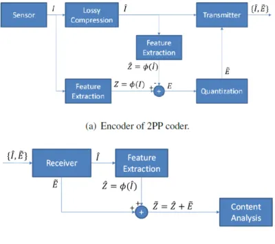
We will now review the design of the Two-Part Predictive (2PP) encoder (Fig. 1.1) and use the same notation presented in [1]. LetI ∈_Rn×m _{be the original}

uncompressed image, ˆI ∈_Rn×m _{be the compressed image, φ(·) :}

Rn×m 7→Rd

be a feature vector extractor that maps I to Z = φ(I) and ˆI to ˆZ = φ( ˆI). Therefore, Z and ˆZ are the feature vectors of I and ˆI, respectively, and

E =Z−Zˆ∈_Rd _{represents the feature error vector due to compression. The}

Figure 1.1: 2PP Encoder and Decoder Architecture

ˆ

I in B1 bits and a quantized feature error vector ˜E, which represents our

predictive feature error, in B2 bits. Hence, our compression ratio is given by

CR= Original Image Size

B1+B2

. (1.1)

The decoder receives the pair of ( ˆI,E˜) from the encoder and restores the compressed image’s feature vector by ˜Z = ˆZ+ ˜E. The goal of this paper is to optimize the quantizer shown in Fig. 1.1 (obtained from [1]). We assess the effectiveness of our quantizer in the classification problem presented in Chapter 3.

1.3

Previous Work: Scalar Lloyd-Max Quantizer

The quantizer used to test the 2PP scheme in [1] was a scalar Lloyd-Max quantizer. Given a desired number of quantization levels K and a set of NT

training examples, a Lloyd-Max quantizer will find theK levels that minimize the sum of the mean squared quantization errors for the particular training data. Lloyd-Max quantization is closely related to k-means clustering in

unsupervised machine learning. More detail regarding the training of a Lloyd-Max quantizer will be given in Chapter 2.

The scalar Lloyd-Max quantizer is trained by performing k-means cluster-ing with K cluster centers on the following list:

E ={Eij|i∈ {1, ..., NT}, j ∈ {1, ..., d}} (1.2)

where Eij is the jth component of the feature error vector Ei =Zi−Zˆi for

the ith _{training example. Each entry in the feature error vector is assigned}

to one of the K quantization levels. Thus, for a feature dimension of d, we use B2 =O(dlogK) bits to encode ˜E.

The scalar Lloyd-Max quantizer recovered a significant amount of classifi-cation accuracy in testing. However, we must use a considerable number of bits to represent the predictive feature errors and reduce the final compres-sion ratio as a consequence. We will discuss these results further in Chapter 3.

1.4

Previous Work: Classification Centric Quantizer

Recent work from Chen and Moulin [2] proposed a vector quantizer referred to as the Classification-Centric Quantizer (CCQ). The goal of the CCQ is to pick an optimal collection of K quantization levels that minimize the L2

norm of the discriminant error vector with respect to a particular classifier. Formally, suppose we have a multiclass classification problem that assigns each test datum to one of Nc classes. The discriminant function for the ith

class is denoted by fi : Rd 7→ R. We may form the discriminant vector for

a particular sample as f~= [f1(Z), f2(Z), . . . , fNc(Z)], whereZ =φ(I) is the

feature vector from image I. The discriminant error vector is then given by the difference between the discriminant vector of the original image and the compressed image received at the decoder:

~

fe(Z) = f~(Z)−f~( ˆZ+ ˜E). (1.3)

The CCQ seeks to minimize the L2 norm of this discriminant error vector.

Fig. 1.1 is:

˜

E =Q(Z, E) = argmin

q∈{q1,...,qK}

kf~(Z)−f~( ˆZ+q)k2. (1.4) To learn an optimal CCQ, we must train a collection of quantization vectors that minimizes the sum of the L2 norms of the discriminant error vectors.

This optimization problem is expressed as

Q= argmin Q0_∈Q K NT X i=1 kf~(Zi)−f~( ˆZi+Q0(Zi, Ei))k2 (1.5)

where QK is the set of all CCQs with any possible combination of K

quan-tization levels each in _Rd. Solving this optimization problem is done using gradient descent methods. Each training example is partitioned by the quan-tizer according to Equation (1.4). Depending on whether Stochastic Gradient Descent (SGD) or Gradient Descent is used, a batch of training examples is used to compute the gradient of the discriminant error vectors with respect to each example’s quantization vector. After each gradient step, the parti-tions are updated such that each training example is reassigned to the best quantization vector. Convergence is observed when the partitions do not change between iterations.

The CCQ improved upon the scalar quantizer presented in [1] by recover-ing similar amounts of classification accuracy while usrecover-ing significantly fewer quantization bits. However, there are a few disadvantages of the CCQ. First, training the CCQ with gradient descent methods takes a considerable amount of time. Results presented in [2] showed that training using SGD for a 25-dimensional (d = 25) quantizer takes on the order of ten minutes. This training time could become troublesome for problems that require a higher dimensionality. Furthermore, training using gradient descent requires knowl-edge of the gradient of a classifier’s discriminant function with respect to the addition of quantization vectors. For classifiers and regression models like Support Vector Machine (SVM) and logistic regression, we can reasonably express the gradient. However, for state-of-the-art classification problems that require neural networks, this gradient becomes intractable. Finally, the optimization problem presented in Equation (1.5) is generally non-convex; therefore, training the CCQ is susceptible to local minima. While gradient

descent may work well, it is not necessarily the best way to find a reason-ably optimal solution. Based on our experiments, proper initialization of the CCQ and tuning of the SGD hyperparameters is important for consistent and effective training. As a result, optimizing the CCQ can be finicky.

CHAPTER 2

THE CLASSIFICATION CENTRIC

LLOYD-MAX QUANTIZER

2.1

Classification Centric Lloyd-Max Quantization

Our proposed refinement of the CCQ is the Classification Centric Lloyd-Max Quantizer (CCLMQ). The CCLMQ is a vector quantizer that is trained by Lloyd’s algorithm (or K-Means clustering) on the set of error vectors{Ei}NTi=1.

Assignment of the quantization vectors is performed with respect to minimiz-ing discriminant vector loss accordminimiz-ing to Equation (1.5), thus maintainminimiz-ing a ”classification centric” aspect to our quantizer.

Training via Lloyd’s algorithm is an iterative process by which we alternate reassignment and re-centering. First, we initialize a cluster center for each of our K quantization levels. Each training example’s feature error vector is assigned to the closest cluster center according to:

Ci = argmin C∈{C1,...,CK}

kEi−Ck22 (2.1)

where Ci is the cluster assignment for the ith training example. After each

training example has been assigned, we re-center each cluster by taking the mean of the feature error vectors belonging to that cluster:

Cj =

P

i∈CjEi NCj

(2.2)

where Cj ∈ Rd is the jth cluster center and NCj is the number of

train-ing examples in the jth cluster. The reassignment and re-centering steps in Equations (2.1) and (2.2) are alternated until the cluster center movement converges. It is important to note again that our cluster centers {Cj}K

j=1

form our quantizer and quantization vector assignments are made like the CCQ according to Equation (1.4).

The CCLMQ enjoys the advantages of the quantizers in both [1] and [2]. The use of a vector quantizer greatly reduces the number of bits B2 used

for the predictive feature errors. Quantization with respect to restoring dis-criminant vectors is well suited to recovering more classification accuracy. Training via Lloyd’s algorithm is both efficient and reliable. The CCLMQ trains remarkably fast compared to the CCQ and optimizing the CCLMQ using K-Means clustering is easy since effective initialization methods like kmeans++ [3] are available. Another distinct advantage of the CCLMQ is that we do not need to use the discriminant function of a classifier to compute gradients during training. We do need the discriminant scores to compute discriminant loss (Equation 1.3); however, this just means we need the output of the classifier instead of a full picture of computation when each example is classified.

The training objective of the CCLMQ is different from the CCQ training objective in that we minimize distances in the feature error space (_Rd₎

in-stead of distance in the discriminant error space (_RNc). Therefore, we train our quantizer in a domain that is different from the domain we evaluate performance in, i.e. we train in the feature domain and evaluate based on classification accuracy, which belongs to the discriminant domain. As such, there are two potential issues with using a distance metric in the feature space:

1. The default metric used in Lloyd’s algorithm is Euclidean distance. However, in many classification problems, we do not have a physical sense of distance and thus a Euclidean metric is potentially poor.

2. As the feature dimensionality increases, clustering in the feature space is sensitive to the curse of dimensionality and we see diminished per-formance.

The speed and reliablility of K-Means clustering gives us room to perform more computation to address these vulnerabilities during training. We ex-plain our corresponding methods of interest, metric learning and Principal Component Analysis (PCA), next.

2.2

Metric Learning for the CCLMQ

The standard Euclidean metric is frequently not the best way to express similarity or distance between two points in an arbitrary vector space. In the case of the CCLMQ, our space of interest is _Rd _{for the feature error}

vectors. There is no guarantee the Euclidean metric is well-suited for this vector space. The goal of metric learning is to generate a distance metric that is most appropriate for a given application or dataset with some kind of guidance or supplementary sense of similarity between points.

In this paper, we will only consider linear metrics, which can be generically represented for some linear operator (matrix) A∈_Rd×d _{as follows:}

dA(x, y) =

p

(x−y)>_{A(x−y). (2.3)}

For example, if we take A = Id×d, we have a representation of Euclidean

distance. The matrix A is commonly referred to as the Mahalanobis matrix of the metric dA(x, y) and can be diagonal or full. We consider the case of a

full A in this paper.

The metric learning algorithm we explore is the distance learning for clus-tering with side information presented in [4]. The side information given to the metric learning algorithm is two distinct sets of similar points S and dissimilar points D. Therefore, we must develop some notion of similarity between feature errors within our training data. As a baseline method, we define similar and dissimilar training examples based on the sign of each en-try in each example’s discriminant error vector. We define a simple transform

φ(f~e(Z)) :Rd 7→Rd on the discriminant error vector as follows:

φ(f~(Z)) = [sgn(fe,1(Z)), ...,sgn(fe,Nc(Z))]. (2.4)

The inner-product between twoφvectors tells us the net sum of entries in the discriminant vectors that agree in sign. Thus,φ(fe~(Zi))>φ(fe~(Zj)) =φ>_i φj ∈ −Nc,−Nc+ 2, . . . , Nc−2, Nc}. To organize pairs of points as similar and

dissimilar, we define the following symmetric rule: (Zi, Zj)∈          S φ>_i φj ≥τ D φ>_i φj ≤ −τ

neither set else

(2.5)

where τ ∈ {τmin, τmin + 2, . . . , Nc −2, Nc} is our similarity threshold and

the minimum value of τ, τmin, is 0 if Nc is even and 1 if Nc is odd. We recognize that a lower threshold gives us more side-information that may also be relatively weak, while a larger threshold gives us less side-information that is likely a stronger indication of truly similar points.

The intuition for this assignment is that we want to cluster training exam-ples together when their classification is similarly degraded by compression, i.e. the entries in their discriminant errors share the same signs. Thus, the objective for training our Mahalanobis metric is well-aligned with the ”classi-fication centric” aspect of our quantizer. We again use K-Means clustering to train the CCLMQ with metric learning; however, we use a modified K-means that can utilize the non-Euclidean metricdA(x, y) =p(x−y)>_{A(x−y). At}

each re-centering step, the new cluster centers are chosen as the point in the cluster with the minimum sum of squared distances to the other points in the cluster. We present results for this baseline method in a high-dimensional case for various values of τ in Chapter 3.

2.3

Principal Component Analysis for the CCLMQ

To address the curse of dimension, we utilize Principal Component Analysis (PCA) to reduce the dimensionality of the space in which we cluster our feature errors. Some methods of metric learning like Relative Component Analysis [5] serve the dual purpose of learning a Mahalanobis metric while reducing dimensionality. In this paper, we consider PCA on its own as a baseline mode of dimensionality reduction in order to separate the potential improvements offered by metric learning and dimensionality reduction.

CHAPTER 3

EXPERIMENTAL SETUP AND RESULTS

3.1

Classification Problem

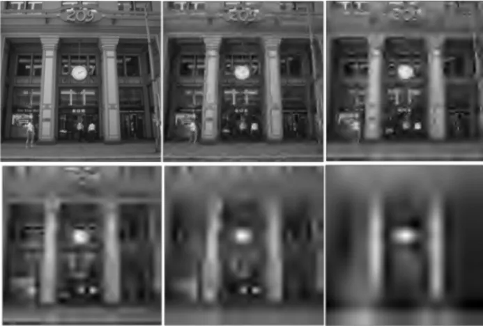
We evaluate the CCLMQ on the Fifteen Scene Categories [6] dataset. We compare classification accuracy on the original image data against the com-pressed image data with different numbers of quantization levels. The images are compressed using JPEG 2000 to specific mean Peak Signal to Noise Ra-tios (PSNR) for consistency with previous work [1][2]. Fig. 3.1 shows an example image from the category ’MITinsidecity’ at various PSNR.

The features collected are dense SIFT visual-word histograms where each 16x16 pixel patch, with a spacing of 8 pixels, is assigned a SIFT descriptor [6]. K-Means clustering is used to come up with d features that form a bag of visual words [6] to describe common textures in each image. The resulting feature vectors are a histogram of counts for each visual word.

We train a One vs. All Support Vector Machine (SVM) for each of the

Nc = 15 classes using the intersection kernel [6]. Given two vectors, the

intersection kernel computes the following scalar:

IK(Zi, Zj) = d

X

k=1

min(Zi[k], Zj[k]) (3.1)

We also use the precomputation techniques presented in [7] to improve the classification time from O(dNsv) toO(dlogNsv), whereNsv is the number of

support vectors for the classifier.

The SVM classifiers are trained using 100 training examples from each cat-egory, while 50 examples are withheld for testing and validation, respectively. The validation examples are particularly important when we employ metric learning as we should avoid overfitting due to the training of the quantizer. The results presented below are the classification accuracies with respect to

Figure 3.1: Example image from ’MITinsidecity’ category. Shown are the original image (top left) and JPEG 2000 compressed images of PSNR 25.9 (top middle), 23.6 (top right), 21.6, 20.3, and 18.4 (bottom row left to right), respectively.

the validation data for consistency between methods.

3.2

Results for 25 Feature Dimensions

Figs. 3.2 and 3.3 show the performance of the CCLMQ against the scalar Lloyd-Max quantizer [1] ford = 25 feature dimensions at varying PSNR and with a specified number of quantization bits B2 used to restore each image’s

feature vector. We see the CCLMQ achieves nearly identical classification accuracy as the scalar quantizer for PSNRs of 25.9 and 21.6 while using far fewer bits for quantization. For every PSNR, the CCLMQ outperforms the scalar Lloyd-Max quantizer by providing similar classification accuracy with fewer quantization bits.

Table 3.1 compares the relative accuracy recoveries of the CCQ [2] and the CCLMQ, respectively. Each entry is the percentage of highest accuracy recovered by each vector quantizer with respect to the highest accuracy of the scalar quantizer [1]. The results for the CCQ are gathered from [2]. The CCLMQ recovers a larger portion of accuracy than the CCQ for every PSNR except 23.6. In summary, atd= 25 feature dimensions, the CCLMQ provides the bit savings of the CCQ, higher relative classification accuracy, trains substantially faster, and requires no knowledge of the classifier’s discriminant function.

Figure 3.2: Classification accuracy vs. compression ratio using scalar Lloyd-Max quantizers [1] with d= 25. Results are presented for varying PSNR after compression and the number next to each point indicates the number of quantization bits used to restore each feature vector.

Figure 3.3: Classification accuracy vs. compression ratio using CCLMQ with d= 25. Results are presented for varying PSNR and number of quantization bits used are labeled next to each point.

Table 3.1: Percentage of accuracy recovered by CCQ and CCLMQ against scalar Lloyd-Max quantizer for d= 25.

Ratio of Highest Accuracies PSNR CCQ CCLMQ 25.9 97.9% 100% 23.6 97.8% 91.4% 21.6 92.5% 98.2% 20.3 86.0% 88.6% 18.4 78.5% 87.7%

3.3

Results for 200 Feature Dimensions

Figs. 3.4 and 3.5 show the performance of the CCLMQ against the scalar Lloyd-Max quantizer [1] for d= 200 feature dimensions as Figs. 3.2 and 3.3 do with respect to d= 25 feature dimensions. We see the CCLMQ is unable to provide the same maximum classification accuracy as the scalar quantizer. However, the CCLMQ still uses far fewer bits at intermediate classification accuracies. For example, at a PSNR of 21.6, the CCLMQ achieves an accu-racy of about 53% using 2 quantization bits while the scalar quantizer uses 400 quantization bits to attain 51% classification accuracy.

Table 3.2 compares the relative accuracy recoveries of the CCQ and the CCLMQ, respectively, like Table 3.1. The CCLMQ consistently underper-forms the CCQ in the d = 200 case on recovered accuracy and we see the largest gap of 14% at a PSNR of 18.4. The CCLMQ is still able to provide the bit savings of the CCQ while training considerably faster; however, we have lower classification accuracy likely due to the curse of dimensionality for the Euclidean metric as mentioned in Chapter 2.

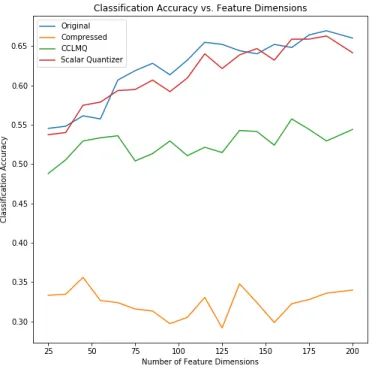
To better inspect this crossover in performance, Fig. 3.6 compares the classification accuracy of the CCLMQ and the scalar quantizer [1] across different feature dimensions at a PSNR of 21.6. The blue and orange lines show the classification accuracy against the original and compressed dataset, respectively. The green and red lines compare the respective classification accuracies of the CCLMQ and scalar quantizer with K = 16 quantization levels. We see the scalar quantizer is able to track the accuracy of the original classifier as the feature dimension increases, while the CCLMQ lags behind.

Figure 3.4: Classification accuracy vs. compression ratio using scalar Lloyd-Max quantizers [1] with d= 200.

Figure 3.5: Classification accuracy vs. compression ratio using CCLMQ with d= 200.

Table 3.2: Percentage of accuracy recovered by CCQ and CCLMQ against scalar Lloyd-Max quantizer for d= 200.

Ratio of Highest Accuracies PSNR CCQ CCLMQ 25.9 96.9% 93.0% 23.6 95.2% 87.5% 21.6 92.0% 84.5% 20.3 90.5% 80.3% 18.4 84.1% 70.4%

Figure 3.6: Classification accuracy vs. feature dimension at PSNR of 21.6 and K = 16 quantization levels. Original and compressed lines show classification accuracy on original and compressed data, respectively.

3.4

Results for CCLMQ + Metric Learning

We examine whether metric learning can improve the performance of the CCLMQ in both the d = 25 and 200 cases and test against a PSNR of 18.4 with K = 16 quantization vectors used. We implement the metric learning algorithm from [4] and provide side information according to Section 2.2. Note that because we have Nc = 15 classes, τ ∈ {1,3, . . . ,13,15}.

Experimentation found that insufficient side information was collected when

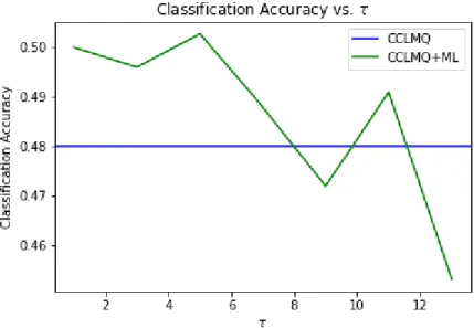
τ = 15 to learn the metric, thus we have omitted that value from testing. Fig. 3.6 shows the classification accuracy of the CCLMQ vs. the CCLMQ + metric learning for various values of τ with K = 16 quantization vectors and d = 25. To be clear, the flat blue line for the CCLMQ represents the classification accuracy of the CCLMQ at a PSNR of 18.4 with 16 quantization vectors. We see a noisy relationship between improvements yielded by metric learning and the amount of side information used. Setting τ = 11 happens to provide a 4% improvement in classification accuracy; however, it is hard to explicitly define whether more or less side information is best to learn a good metric.

Fig. 3.7 again shows the classification accuracy of the CCLMQ vs. the CCLMQ + metric learning like Fig. 3.6, except with d= 200 feature dimen-sions. We see that the use of metric learning provides a modest improvement of around 2% accuracy when τ =1, 3, or 5. Interestingly, we observe a rough trend that suggests a lower similarity threshold outperforms a higher thresh-old in this case. This means we learn a better metric with larger amounts of side information that represent weaker similarities and dissimilarities. Larger thresholds likely provide too little side information and the information that is provided poorly describes the data.

In summary, it is difficult to discern the benefits of metric learning from these results. There is no consistent relationship between the d = 25 and 200 cases with improvements due to metric learning and the nature of the provided side information. As we discuss in the conclusion in Chapter 4, future work should further explore the potential of metric learning.

Figure 3.7: Classification accuracy vs. τ for CCLMQ + metric learning with d= 25, K = 16 quantization vectors, and PSNR of 18.4. The flat blue line represents the classification accuracy of the CCLMQ in the same context with K = 16 quantization vectors.

Figure 3.8: Classification accuracy vs. τ for CCLMQ + metric learning with d= 200, K = 16 quantization vectors, and PSNR of 18.4.

3.5

Results for CCLMQ + PCA

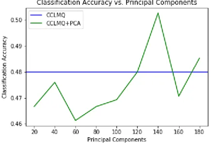
We also examine whether Principal Component Analysis (PCA) helps the CCLMQ with the curse of dimensionality to improve classification accuracy. Fig. 3.8 shows the classification accuracy of the CCLMQ vs. the CCLMQ + PCA for several numbers of principal components whered= 200. Consistent with the previous section, we again test with a PSNR of 18.4. The use of PCA also provides a modest improvement to the CCLMQ. The results are noisy; however, we see that keeping 140 principal components out of the

d = 200 dimensions strikes a balance that provides a 2% improvement in classification accuracy.

Figure 3.9: Classification accuracy vs. number of principal components for CCLMQ + PCA with d= 200, K = 16 quantization vectors, and PSNR of 18.4. The flat blue line represents the classification accuracy of the

CHAPTER 4

CONCLUSION

We have proposed the Classification Centric Lloyd-Max Quantizer (CCLMQ) as a vector quantizer alternative to the Classification Centric Quantizer [2] for the Two Part Predictive (2PP) encoder. The CCLMQ allows for rapid quantizer training and relaxes the requirement of the CCQ to be able to compute gradients of a classifier’s discriminant function. We saw in a lower dimensional d= 25 case that the CCLMQ also repeatedly outperformed the CCQ on classification accuracy. In the higher dimensional d = 200 case, the CCLMQ recovered less classification accuracy than the CCQ, but still provided quantization bit savings over scalar Lloyd-Max quantizers [1] at the same classification accuracy. Baseline results using metric learning with discriminant-based side information and dimensionality reduction using PCA each yielded improved results for the CCLMQ.

Future work could explore the potential of metric learning and dimension-ality reduction to continue to improve the CCLMQ. Our selection rule for side information in Equation 2.2 could be modified to not only take into ac-count discriminant error vector signs, but also the magnitudes of each entry, for example. The metric learning algorithm used [4] was chosen as a baseline to build a linear metric. Other metric learning algorithms, linear and poten-tially non-linear, should be considered. The results presented in Sections 3.4 and 3.5 should motivate further examination of refinements to the CCLMQ.

REFERENCES

[1] S. D. Chen and P. Moulin, “A two-part predictive coder for multitask sig-nal compression,” in 2014 IEEE International Conference on Acoustics,

Speech and Signal Processing (ICASSP), May 2014, pp. 2035–2039.

[2] S. D. Chen and P. Moulin, “A classification centric quantizer for efficient encoding of predictive feature errors,” in2014 48th Asilomar conference

on Signals, Systems and Computers, Nov. 2014, pp. 2098–2102.

[3] D. Arthur and S. Vassilvitskii, “K-means++: The advantages of careful seeding,” in Proceedings of the Eighteenth Annual ACM-SIAM

Symposium of Discrete Algorithms. Philadelphia, PA, USA: Society

for Industrial and Applied Mathematics, 2007. [Online]. Available: http://dl.acm.org/citation.cfm?id=1283383.1283494 pp. 1027–1035. [4] E. P. Xing, M. I. Jordan, S. J. Russell, and A. Y. Ng, “Distance metric

learning with application to clustering with side-information,” in

Ad-vances in neural information processing systems, 2003, pp. 521–528.

[5] A. Bar-Hillel, T. Hertz, N. Shental, and D. Weinshall, “Learning dis-tance functions using equivalence relations,” inProceedings of the Twen-tieth International Conference on International Conference on Machine

Learning, ser. ICML’03. AAAI Press, 2003, pp. 11–18.

[6] S. Lazebnik, C. Schmid, and J. Ponce, “Beyond bags of features: Spa-tial pyramid matching for recognizing natural scene categories,” in2006 IEEE Computer Socieity Conference on Computer Vision and PAttern

Recognition (CVPR’06), 2006, pp. 2169–2178.

[7] S. Maji, A. C. Berg, and J. Malik, “Classification using intersection ker-nel support vector machines is efficient,” in 2008 IEEE Conference on