OUTPUT, INPUT AND PRODUCTIVITY MEASURES AT
THE INDUSTRY LEVEL: THE EU KLEMS DATABASE*
Mary O’Mahony and Marcel P. Timmer
This article describes the contents and the construction of the EU KLEMS Growth and Productivity Accounts. This database contains industry-level measures of output, inputs and productivity for 25 European countries, Japan and the US for the period from 1970 onwards. The article considers the methodology employed in constructing the database and shows how it can be useful in comparing productivity trends. Although growth accounts are the organising principle, it is argued that the database is useful for a wider range of applications. We give some guidance to prudent use and indicate possible extensions.
Internationally comparable studies of the relationships between skill formation, investment, technological change and growth have been hampered up to now by the lack of a readily available standard database covering a large set of countries. As a result, researchers had often to compile their own databases, making replication and com-parability of studies difficult. This article describes the construction of a new database which can serve as a useful tool for empirical and theoretical research in the area of economic growth: the EU KLEMS Growth and Productivity Accounts. This database includes measures of output and input growth, and derived variables such as multi-factor productivity at the industry level. The input measures include various categories of capital (K), labour (L), energy (E), material (M) and service inputs (S). The mea-sures are developed for 25 individual EU member states, the US and Japan and cover the period from 1970 to 2005. The variables are organised around the growth accounting methodology, a major advantage of which is that it is rooted in neo-classical production theory. It provides a clear conceptual framework within which the inter-action between variables can be analysed in an internally consistent way.
The data series, publicly available on http://www.euklems.net, can be used by researchers employing growth accounting to consider sources of output and pro-ductivity growth in cross-country comparisons or studies of particular industries and different time periods, such as in Jorgensonet al.(2005) for the US and van Arket al. (2008) for Europe versus the US. Although the primary aim of the EU KLEMS database is to generate comparative productivity trends, the data collected are also useful in a large number of other contexts, as the EU KLEMS database provides many basic input data-series. These input series are derived independently from the assumptions underlying the growth-accounting method. Due to its wide country and industry coverage, potential applications of the database vary widely. For example, * This research was supported by the European Commission, Research Directorate General as part of the 6th Framework Programme, Priority 8,!Policy Support and Anticipating Scientific and Technological Needs" and is part of the!EU KLEMS project on Growth and Productivity in the European Union". The project was carried out by a consortium of 24 research institutes and national statistical institutes (see Appendix 1 for list). We are grateful to all participants in the EU KLEMS consortium for their contribution without which the construction of this database would have been impossible. The article has also benefited from comments from two anonymous referees
there has been considerable research on the issue of whether technical change is skill-biased and on the impact of information and communications technology (ICT) on the demand for skilled labour (e.g. Autor et al., 1998; Machin and van Reenen, 1998). Typically researchers estimate wage share equations by labour type and include a variable measuring some aspect of technological change. EU KLEMS is likely to be useful in such exercises as the database contains information on hours and wage bill shares cross-classified by skill, gender and age and provides a breakdown of capital into ICT and non-ICT assets. EU KLEMS data can also be combined with data from other sources to consider relationships between competition, education, R&D, innovation and growth (examples include Griffith et al., 2004; Aghion et al., 2005; Vandenbussche et al., 2006; Aghion and Griffith, 2005; Inklaar et al., 2008). More broadly, the database allows evaluation of various monetary, tax, innovation, com-petition and other industrial policies. And it might be used in studies of international specialisation and outsourcing (along the lines of, for example, Harrigan (1997) and Antr!as and Helpman (2004) to name but a few) as well as studies of income inequality and wage setting (Koeniger and Leonardi, 2007). Frequently, due to a lack of data, many of these studies rely on industry panels. However this raises some serious issues of interpretation since many relationships are known to vary across industries. The EU KLEMS database with its rich data across countries allows for the first time estimations industry-by-industry so that the cross-section panel dimension in the data is country, rather than industry.
As with any resource, users need to understand the theoretical and practical underpinnings of the database in order to optimise the research benefit. The main purpose of this article is therefore to summarise the methodology employed in con-structing the database and so guide researchers on appropriate uses. Naturally this requires that we also consider the practical limitations of the database and indicate areas for further improvement. In addition we illustrate the usefulness of the database by highlighting some interesting findings on trends and levels of productivity in Eur-ope relative to the US.
The remainder of this article is organised as follows. Section 1 considers theoretical and practical measurement issues and summarises data sources. Section 2 describes trends in productivity and input use in Europe and the US and considers relative productivity levels. Section 3 is essentially a user’s guide, summarising what is in the dataset, and outlines issues related to the use of the database in both growth accounting and econometric analysis. This Section ends with some health warnings. The EU KLEMS database is a dynamic resource that will be added to and revised over time. Section 4 considers future developments, those already planned and suggestions on ways forward in the longer term.
1. Theory and Measurement Issues
This Section considers the measurement of output and productivity growth both in theory and practice. It begins with an outline of the growth accounting method which is the organising principle underlying the construction of the database. However it is important to emphasise that much of EU KLEMS is a resource independent of this method as many basic input series are provided as well.
1.1.Theoretical Background
To assess the contribution of the various inputs to aggregate economic growth, we apply the growth accounting framework. This methodology has been theoretically motivated by the seminal contribution of Jorgenson and Griliches (1967) and put in a more general input–output framework by Jorgensonet al. (1987). It is based on pro-duction possibility frontiers where industry gross output is a function of capital, labour, intermediate inputs and technology, which is indexed by time, T. Each industry, indexed by j, can produce a set of products and purchases a number of distinct intermediate inputs, capital and labour inputs to produce its output. The production function is given by:
Yj ¼fjðKj;Lj;Xj;TÞ ð1Þ
whereYis output,Kis an index of capital service flows,Lis an index of labour service flows and X is an index of intermediate inputs, either purchased from domestic industries or imported. Under the assumptions of competitive factor markets, full input utilisation and constant returns to scale, the growth of output can be expressed as the cost-share weighted growth of inputs and technological change (AY), using the translog functional form common in such analyses:1
DlnYjt¼v"jtXDlnXjtþv"jtKDlnKjtþv"LjtDlnLjtþDlnAYjt ð2Þ
wherev"i denotes the two-period average share of inputiin nominal output defined as
follows: vX jt ¼ PX jtXjt PY jtYjt ; vL jt ¼ PL jtLjt PY jtYjt ; vK jt ¼ PK jtKjt PY jtYjt ð3Þ
and v"L þv"K þv"X ¼ 1. Each element on the right-hand side of (2) indicates the
proportion of output growth accounted for by growth in intermediate inputs, capital services, labour services and technical change as measured by multifactor productivity (MFP), respectively. It is common to define aggregate input, say labour, as a To¨rnqvist quantity index of individual labour types as follows:2
DlnLjt¼ X l " wlL;jtDlnLl;jt ð4Þ DlnKjt¼ X k " wKk;jtDlnKk;jt ð5Þ DlnXjt¼ X x " wxX;jtDlnXx;jt ð6Þ 1
To be more precise, A reflects Hicks-neutral technical change. Because of our approach to capital measurement it only includes disembodied technical change, see also the discussion in Section 3.2.4.
2Aggregate input is unobservable and it is common to express it as a translog function of its individual components. Then the corresponding index is a To¨rnqvist volume index (see Jorgensonet al., 1987).
whereDlnLl,t indicates the growth of hours worked by labour typeland weights are
given by the period average shares of each type in the value of labour compensation, and similarly forKandX. As we assume that marginal revenues are equal to marginal costs, the weighting procedure ensures that inputs which have a higher price also have a larger influence in the input index. So for example a doubling of hours worked by a high-skilled worker gets a bigger weight than a doubling of hours worked by a low-skilled worker.
For many analyses it is useful to subdivide total intermediate inputs into three groups: energy, materials and services (E,M,S) such that:
DlnXjt¼w"EjtDlnXjtEþw"jtMDlnXjtM þw"jtSDlnXjtS: ð7Þ
Withw"E
jt the period-average share of energy products in total intermediate input costs
in industryjattand similarly for materials and services. Input volume growth ofE,M andSare defined in terms of their components as
DlnXjtE ¼X xeE " wEx;jtDlnXx;jt ð8Þ DlnXjtM ¼X xeM " wxM;jtDlnXx;jt ð9Þ DlnXjtS ¼X xeS " wxS;jtDlnXx;jt ð10Þ withw"E
x;jt the period-average share of productxin total energy costs in industryjatt,
and similarly for materials and services.
To analyse the separate impact of ICT and non-ICT capital, we divide capital input growth into two groups of assets: ICT (ICT) and non-ICT (N) assets, such that:
DlnKjt¼w"jtICTDlnKjtICT þw"jtNDlnKjtN ð11Þ
withw"ICT
jt the period-average share of ICT assets in total capital costs in industryjatt,
and similarly for non-ICT assets. Volume growth of ICT and non-ICT are defined as:
DlnKICT jt ¼ X keICT " wICT k;jt DlnKk;jt ð12Þ DlnKjtN ¼X keN " wkN;jtDlnKk;jt ð13Þ withw"ICT
k;jt the period-average share of ICT-assetkin total ICT-capital costs in industry
jand similarly for non-ICT assets.
In terms of labour inputs, it is useful to split the volume growth of labour input into the growth of hours worked and the changes in labour composition in terms of labour characteristics such as educational attainment, age or gender (see below). Let Hl,jt
worked by all types (summed over l) then we can decompose the change in labour input as follows: DlnLjt ¼ X l wl;jtDln Hl;jt Hjt þDln Hjt¼DlnLCjtþDlnHjt ð14Þ
withw"l;jt the period-average share of labour type lin total labour costs in industry j.
The first term on the right-hand side indicates the change in labour composition and the second term indicates the change in total hours worked.3 It can easily be
seen that if proportions of each labour type in the labour force change, this will have an impact on the growth of labour input beyond any change in total hours worked.4
Using the above formulas, the EU KLEMS database provides a full decomposition of growth in gross output into eight elements as follows:
DlnYjt ¼v"Xjtw"jtEDlnXjtEþv"jtXw"jtMDlnXjtM þv"Xjtw"jtSDlnXjtS
þv"jtKw"jtICTDlnKjtICTþv"jtKw"NjtDlnKjtN þv"jtLDlnLCjtþv"jtLDlnHjt þDlnAYjt:
ð15Þ
The contribution of each intermediate and capital input is given by the product of its share in total costs and its growth rate. The contribution of labour input is split into hours worked and changes in the composition of hours worked, and any remaining output growth is picked up by the multi-factor productivity termA. This term is also known astotalfactor productivity. An example of the application of this methodology is discussed in Section 3.1.
Finally the EU KLEMS database also includes estimates of productivity levels. Com-paring productivity levels across countries is in many ways analogous to comparisons over time. However, while one typically compares productivity in one year with pro-ductivity in the previous year, there is no such natural ordering of countries. Therefore the comparison should not depend on the country that is chosen as the base country. There are various index number methods that can be used to make multilateral comparisons. We use the method suggested by Caveset al.(1982). This index mirrors the To¨rnqvist index approach used in our growth accounting, but all countries are compared to an artificial!average"country (AC), defined as the simple average of allN countries in the set. Gaps in multi-factor productivity levels can be derived by sub-tracting the compensation-weighted relative inputs from relative output as follows (industry and time subscript suppressed for convenience):
3The first term is also known as!labour quality"in the growth accounting literature (see e.g. Jorgenson
et al.2005). However, this terminology has a normative connotation which easily leads to confusion. For
example, lower female wages would suggest that hours worked by females have a lower!quality"than hours worked by males. Instead we prefer to use the more positive concept of!labour composition".
4The growth accounting calculations in EU KLEMS included this division into volume and composition for labour input to summarise all aspects of labour composition. Alternatively, in keeping with the divisions for intermediate and capital input one could subdivide the contribution of labour into groups, e.g. high-skilled and low-high-skilled labour. The data necessary for such a division is also available in the database – see below for further details.
ln A Y c AY AC ¼ln Yc YAC% " vXln Xc XAC % " vKln Kc KAC % " vLln Lc LAC ð16Þ
withvs the input shares in gross output averaged between country" c and the average country AC. A comparison between two countries, say Germany and the US, can be made indirectly: by first comparing each country with the average country and then comparing the differences in German and US levels relative to the average country. Inklaar and Timmer (2008) provide further discussion.
1.2.Practical Implementation
The EU KLEMS database has largely been constructed on the basis of data from national statistical institutes (NSIs) and processed according to harmonised proce-dures. These procedures were developed to ensure international comparability of the basic data and to generate growth accounts in a consistent and uniform way. Cross-country harmonisation of the basic country data has focused on a number of areas including a common industrial classification and the use of similar price concepts for inputs and outputs but also consistent definitions of various labour and capital types. Importantly, this database is rooted in statistics from the National Accounts and follows the concepts and conventions of the System of National Accounts (SNA) framework, and its European equivalent (ESA), in many respects. As a result, the basic statistics within EU KLEMS can be related to the national accounts statistics published by NSIs, although with adjustments that vary by group of variables: output and intermediate inputs, labour input and capital input. This will be discussed in more detail below.
Nominal and price series for output and total intermediate inputs at the industry level are taken directly from the National Accounts. As these series are often short (as revisions are not always taken back in time) different vintages of the national accounts were bridged according to a common link-methodology. In cases where industry detail was missing additional statistics from censuses and surveys were used to fill the gaps. Series on intermediate inputs are broken down into energy, materials and services based on supply-and-use tables using a standardised product classification. To ensure consistency with the national accounts series, proportions of energy, materials and services inputs were applied to the total intermediate input series from the National Accounts.
Labour service input is based on series of hours worked and wages of various types of labour. These series are not part of the core set of National Accounts statistics put out by NSIs; typically only total hours worked and wages by industry are available from the National Accounts. For these series additional material has been collected from employment and labour force statistics. We cross-classify hours worked by educational attainment, gender and age (to proxy for work experience) into 18 labour categories (respectively 3&2&3 types). For each country covered, a choice was made of the best statistical source for consistent wage and employment data at the industry level. In most cases this was the labour force survey (LFS), which in some cases was combined with earnings surveys when wages were not included in the LFS. In other instances, an establishment survey, or social-security
database was used (Timmer et al., 2007). Care has been taken to arrive at series which are time consistent, as most employment surveys are not designed to track developments over time and breaks in methodology or coverage frequently occur. Labour compensation of self-employed is not registered in the National Accounts, which, as emphasised by Krueger (1999), leads to an understatement of labour’s share. We make an imputation by assuming that the compensation per hour of self-employed is equal to the compensation per hour of employees. This is especially important for industries which have a large share of self-employed workers, such as agriculture, trade, business and personal services. Also, we assume the same labour characteristics for self-employed as for employees when information on the former is missing. These assumptions are made at the industry level.
Capital input series by industry are generally not available from the National Accounts. At best, capital stocks are estimated for aggregate investment without dis-tinguishing various asset types. In EU KLEMS, capital input is measured as capital services, rather than stocks. It has been measured as the weighted growth of stocks of eight assets as in (11)–(13).5The weights are based on the rental price of each asset
which consists of a nominal rate of return, depreciation and capital gains.6 The nominal rate of return is determined ex post as it is assumed that the total value of capital services for each industry equals capital compensation. Capital compensation is derived as gross value added minus labour compensation. This procedure yields an internal nominal rate of return that exhausts capital income and is consistent with constant returns to scale. The nominal rate of return is the same for all assets in an industry but is allowed to vary across industries.
For each individual asset, stocks have been estimated on the basis of investment series using the perpetual inventory method (PIM) with geometric depreciation pro-files. Depreciation rates differ by asset and industry but have been assumed identical across countries. Appendix B provides more details on capital service calculations. The basic investment series by industry and asset have been derived from capital flow matrices and benchmarked to the aggregate investment series from the National Accounts. Although the ESA provides a classification of capital assets, it is not always detailed enough to back out investment in information and communication equip-ment. Additional information has been collected to obtain investment series for these assets, or assumptions concerning hardware-software ratios have been employed. When the deflator for computers did not contain an adjustment for quality change, a harmonised deflator based on the US deflator has been used as suggested by Schreyer (2002).
The EU KLEMS database provides data at a detailed industry level but also provides higher level aggregates, such as the total economy, the market economy, total market services and total goods production for all variables. All aggregations of output and input volumes across industries use the To¨rnqvist quantity index. For example, the growth rate of total economy capital services is given as a weighted average of capital services growth across industries as follows:
5
These assets are residential structures, non-residential structures, transport equipment, information technology equipment, communication technology equipment, other machinery and equipment, software and other fixed capital assets.
DlnKt¼ X j " uK jtDlnKjt ð17Þ withu"K
jt the period-average share of industryjin total economy capital compensation.
Similar industry aggregations are used for labour and value added. This is akin to the
!direct aggregation across industries"approach as developed by Jorgensonet al.(1987, ch. 2). It is based on the assumption that value-added functions exist for each industry but does not impose cross-industry restrictions on either value-added or inputs. This approach allows us to trace the source of aggregate growth to the underlying industry sources explicitly.7
Aggregations are also made across countries. To do so use is made of industry-specific Purchasing Power Parities (PPPs) which reflect differences in output price levels across countries at a detailed industry level. The PPPs are given for the bench-mark year 1997. PPPs are also needed to adjust output and inputs for differences in relative price levels between countries in levels comparisons. This price adjustment is often done by means of GDP PPPs which reflect the average expenditure prices in one country relative to another and are widely available through the work of the OECD and Eurostat. However, it is well recognised that the use of GDP PPPs, which reflect expenditure prices ofallgoods and services in the economy, can be misleading when used to convert industry-level output. The EU KLEMS database makes use of a new and comprehensive dataset of industry PPPs for 1997, in combination with a benchmark set of Supply and Use tables. PPPs for value added are constructed by double deflation of gross output and intermediate inputs within a consistent input-output framework. In addition, relative price ratios for labour and capital input are developed – for details see Inklaar and Timmer (2008). Level estimates are discussed also in Section 3 below. 1.3.Comparison with OECD STAN
Empirical implementation of the growth-accounting methodology for European countries has been scarce. Despite the publication of an OECD handbook on pro-ductivity measurement (Schreyer, 2001), which is based on the growth accounting methodology, national statistical institutes (NSIs) have been slow in adopting this methodology and, to date, only one European NSI, i.e. Statistics Denmark, has pub-lished MFP-measures on a regular basis.8The OECD and the Groningen Growth and Development Centre maintain MFP series for OECD economies but not at the industry level.9
Because of the lack of useful statistics, various scholars have based their analysis on the OECD Structural Analysis database (STAN) and its predecessor the International
7See Jorgensonet al.(2005, ch. 8) for an elaborate discussion.
8Several European NSIs are experimenting with growth accounting statistics, including Statistics Neth-erlands, Statistics Sweden, Statistics Finland and ISTAT (the Italian NSI). Outside Europe, the Australian Bureau of Statistics, Statistics Canada and the US Bureau of Labor Statistics (BLS) maintain a detailed productivity programme.
9For OECD productivity programme, see http://www.oecd.org. For GGDC series, see Total Economy Growth Accounting database at www.ggdc.nl, described in Timmer and van Ark (2005). Also see O’Mahony (1999) and Inklaaret al. (2005) for international comparisons at the industry-level for a limited set of countries.
Sectoral Database (ISDB). Interestingly, these databases were never designed for pro-ductivity analysis and as a result researchers had to apply additional methods and make ad hocadjustments, for example in the calculation of capital stocks.10 This was done
mostly for the purpose of one single study, which hindered validation and replication of results by others. The OECD STAN database provides industry-level series on output, employment and aggregate investment for OECD member states. For a limited number of countries, capital stocks are given as well. It is almost exclusively based on data published in the latest vintage of the National Accounts of each country. In addition, EU KLEMS uses additional sources such as earlier vintages of the National Accounts, industry surveys, labour force surveys and capital formation surveys. While essentially complementary in many respects, the EU KLEMS database goes beyond STAN by providing:11
' Long historical time series
' Breakdown of industries to a common level of industry detail
' A breakdown of intermediate inputs into energy, materials and services ' A breakdown of hours worked by type of worker
' A breakdown of investment into various asset types
' Calculation of capital stocks and services using a harmonised methodology ' Estimates of multi-factor productivity (MFP) based on growth accounting Productivity measures based on aggregate concepts of inputs as in STAN can be seriously biased. The EU KLEMS database shows that there is a general shift towards more skilled and more experienced workers in the labour force. As such, labour ser-vices grow faster than suggested by a crude measure of hours worked, unadjusted for changes in labour composition. Similarly, especially in the past decade, the importance of short-lived ICT assets relative to non-ICT assets has increased. Consequently, capital service input growth rates are higher than capital stock growth rates as ICT assets deliver more services per unit of capital stock. Not accounting for this shift in the composition of capital biases input measures downwards, and consequently MFP measures upwards.
In general, one can say that the differences in labour productivity growth rates between STAN and EU KLEMS are relatively minor, underlying the complementary nature of the two databases for basic data. This is useful since STAN provides data for some OECD countries not yet in EU KLEMS plus additional information on trade flows. Differences in output and employment growth are generally negligible, although differences in estimates of hours worked might be bigger (see also Section 3.2).12The greatest difference can be found in capital stock estimates. STAN provides aggregate stock estimates for those countries which publish these in their National Accounts. The internationally harmonised approach to capital measurement in EU KLEMS often
10
Instead STAN was intended for tracking knowledge spillovers (in combination with other OECD data-bases such as ANBERD and the input-output database) and general structural analyses.
11 STAN includes a number of variables not included in EU KLEMS, most notably imports and exports by product group.
12 Possible differences are due to differences in the vintage on the National Accounts series used and in the use of different index-number formulae for industry-aggregation. We use the theoretically based To¨rnqvist indices, whereas in most National Accounts and in STAN chained Laspeyres type indices are used. These differ only in cases of very high or low growth rates.
differs from the practice used in the National Accounts of a particular country. In addition, EU KLEMS provides estimates of the changes in the composition of the capital stock and in the labour force, which cannot be derived with the STAN database. In Table 1 we illustrate the differences between input and productivity growth rates based on EU KLEMS and those based on STAN for a particular sector (distributive trade) and for those countries for which STAN has capital stock estimates (Germany, Italy, Spain and the US). Indeed, differences in labour productivity growth rates (value added per hour worked) are generally small. But differences in the capital stock estimates can be sizeable due to the different methodologies employed. The adjustments for capital and labour composition in EU KLEMS provide additional information not available in STAN.13
In addition to improving MFP estimates, detailed data on various input types are useful in their own right. They can for example be used in studies of energy efficiency, services outsourcing, skill formation and skill premia and investment in ICT assets.
2. Growth and Productivity in Europe, Japan and the US
The data provided in the EU KLEMS database can be used for the study of a variety of issues. In this Section we highlight some interesting findings in an analysis of productivity growth and level differences across Europe, Japan and the US focusing on the market economy.14
Since the mid-1990s, labour productivity growth in most European countries has significantly slowed compared to earlier decades. In contrast, labour productivity growth in the US accelerated, so that a new productivity gap has opened up. On the basis of EU KLEMS data, van Ark et al. (2008) argue that this is attributable to the slower emergence of the knowledge economy in Europe over the period 1995–2004. When looking at the growth accounts from the perspective of the emerging knowledge
Table 1
EU KLEMS and STAN Estimates of Productivity Growth, Distributive Trades, 1995–2004 (annual average volume growth rates, in %)
Germany Italy Spain UnitedStates STAN EUK STAN EUK STAN EUK STAN EUK Labour productivity growthof which contribution by 1.9 1.9 0.9 0.9 0.2 0.6 4.6 4.4
capital stock growth 0.7 0.5 2.9 1.3 1.2 0.8 1.2 0.9
changes in capital composition – 0.1 – 0.2 – 0.3 – 0.2
changes in labour composition – 0.0 – 0.5 – 0.4 – 0.3
MFP growth (value added based) 1.2 1.3 %2.0 %1.1 %1.0 %0.9 3.4 3.1
Notes. Contributions of factor inputs are calculated as the share of input times the growth rate, in percentage
points.
Source. STAN estimates based on OECD,STAN database, release March 2008. EUK fromEU KLEMS database,
release March 2008, see Timmeret al.(2007). Figures might not add due to rounding.
13
See Inklaaret al.(2008) for a discussion of the sensitivity of results to alternative productivity measures in the context of a study on the impact of regulation and skilled labour on productivity catch up.
14 Market economy in EU KLEMS excludes the real estate sector, public administration and education, health and social services, due to problems in measuring productivity in these sectors, see Section 4.2.
economy, they focus on the summed contributions of three factors: direct impacts from investments in information and communication technology, changes in labour com-position mostly driven by greater demand for skilled workers and multifactor pro-ductivity growth, which includes the impact of innovation and intangible investments such as organisational changes related to the use of ICT. Table 2 reproduces the calculations underlying their findings, updated to 2005 and including some additional European Union countries and Japan. The first column of Table 2 shows the growth rate of output in the market economy of 16 European countries, the EU total, Japan and the US between 1995 and 2005. The second and third columns divide that growth into changes in hours worked and changes in output per hour – or labour productivity. Columns 4–7 divide up the growth in labour productivity into four factors: changes in labour composition, investments in ICT, other types of investments and multifactor productivity. The final column in Table 2 shows the !knowledge economy" contribu-tions as defined above and highlights the discrepancy between growth in Europe and the US noted by van Arket al.(2008).
One key observation to be drawn from this Table is that the main difference in labour productivity growth between individual European economies and the US is to be found in multifactor productivity, not in differences in the intensity of the pro-duction factors. For the EU as a whole, the labour productivity growth gap is 1.4 percentage points of which 0.9 can be explained by lower MFP growth in the EU. Lagging ICT investments explains only 0.4 percentage points of the growth-gap, while growth differences in non-ICT capital per hour and in labour services per hour are negligible. The same story holds for most European countries. Similarly, the sources of labour productivity growth in Japan are very similar to those in the EU, except that employment growth in Japan was negative.
Within Europe, there is also a divergence of labour productivity growth rates. This is not so much due to differences in input growth rates. In particular, in all countries there have been positive contributions of changes in labour composition and from investment in ICT. Instead differences in multifactor productivity seem to have driven the divergence across Europe. In Belgium, Denmark and Germany, MFP growth is below 0.5% per year and in Italy, Czech Republic and Spain it is even negative. In contrast, MFP growth in Finland, Hungary and Ireland is around 3%. Note in the case of these countries, MFP also captures some element of conventional catch-up growth as they lagged relatively far behind the rest in 1995.
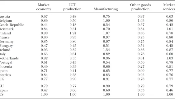
When analysing cross-country patterns, growth accounts provide only a partial analysis. It is now widely accepted that understanding the pattern of cross-country growth and productivity requires estimates of relative levels. For example, studies on the impact of differences in education, research and development or market regulation across countries rely heavily on level measures of MFP which indicate the distance to the technology frontier.15Inklaar and Timmer (2008) provide new productivity level estimates which complement the EU KLEMS growth accounts. Table 3 shows relative MFP levels for the market economy and a division of this into four sectors: ICT goods and services production, manufacturing, other goods production and market services.
15 See e.g. Cameronet al.(2005), Griffithet al.(2004), Nicoletti and Scarpetta (2003), Vandenbusscheet al. (2006) and Inklaaret al.(2008).
Table 2 Gross Value Added Growth and Contributions, 1995–2005, Market Economy Growth rate of value added Value contr ibution added from Labou r produ ctivity contr ibutions fr om La bour produc tivity con tribution of the knowl edge econom y Hour s wor ked Labo ur produ ctivity Labour comp osition ICT capi tal per hour Non-ICT capita l p er ho ur M ulti factor produc tivity 1 ¼ 2 þ 32 3 ¼ 4 þ 5 þ 6 þ 74 5 6 7 4 þ 5 þ 7 Austria 2.5 0.5 2.0 0.2 0.6 0.2 1.1 1.9 Belgium 2.3 0.7 1.7 0.2 1.0 0.6 0.1 1.3 Czech Rep ublic 1.5 % 0.7 2.1 0.1 1.1 1.7 % 1.1 0.1 Denma rk 2.2 0.7 1.6 0.2 1.1 0.4 0.0 1.3 Finland 4.3 1.1 3.2 0.1 0.7 0.2 2.5 3.2 France 2.4 0.4 2.1 0.4 0.4 0.5 0.8 1.6 Germany 1.0 % 0.6 1.5 0.1 0.5 0.5 0.4 0.9 Hunga ry 4.3 1.6 2.7 0.1 0.0 0.1 2.7 2.9 Irelan d 9.7 4.5 5.2 0.2 0.8 3.7 2.0 3.0 Italy 1.2 0.9 0.3 0.2 0.3 0.8 % 0.7 % 0.2 Netherlands 2.8 0.7 2.1 0.4 0.6 0.3 1.0 2.0 Portugal 3.9 1.0 3.0 % 0.4 0.9 1.9 0.8 1.3 Sloveni a 4.3 % 1.0 5.3 0.3 0.5 2.1 1.4 2.2 Spain 3.6 3.2 0.4 0.4 0.5 1.4 % 0.8 0.0 Swede n 4.4 1.2 3.2 0.1 0.8 1.5 1.0 2.0 UK 3.2 0.6 2.6 0.5 0.9 0.6 0.9 2.3 EU 2.2 0.7 1.5 0.2 0.6 0.6 0.4 1.2 Japan 1.0 % 1.7 2.6 0.4 0.5 0.6 0.5 1.3 US 3.6 0.7 2.9 0.3 1.0 0.5 1.3 2.7 Notes . Growth rates ar e annu al ave rage vol ume grow th ra tes. Con tributions in perc entage points . Figures mi ght no t add d ue to roundi ng. Europea n Union is (weight ed) average of the old EU-15 coun tries sho wn in the Table. Author s " calculations based on E UKLEMS dat abase , relea se March 2008, see Timme r et al. (2007).
These estimates suggest that in 2005 the US had a significant MFP lead over all European countries. Relative MFP in the EU is only 79% of the US. This gap is mainly in market services, ICT production and other goods production (around 80%), rather than in manufacturing (90%). In fact, in manufacturing MFP levels in 2005 in some countries are close to the US or even above, including Belgium, Finland, France, Germany, Ireland and Netherlands. In contrast, in market services significant pro-ductivity gaps with the US exist in almost all European countries, in particular Italy. In Japan large gaps are to be found in both manufacturing and market services.
Figure 1 traces the developments of relative input and productivity levels in the European market economy over the period 1980–2005 by extrapolating the level esti-mates with growth rates from the EU KLEMS database. Up to the mid-1990s labour productivity in Europe caught up with the US, continuing the long-term trend since the Second World War. This narrowing of the labour productivity gap was mainly due to higher investment in Europe than in the US. Capital intensity levels increased from about 82% of the US level in 1980 to 95% in 1995, while relative MFP levels remained more or less constant. This period of rapid capital intensification was primarily related to the high wage/rental ratios in Europe compared to the US (van Arket al., 2008). This trend reversed in the mid-1990s as investment in ICT in the US soared and relative cost of labour in the EU countries declined due to policies to raise the employment rate. At the same time the MFP gap between the EU and the US widened which, as implied by Table 3, is concentrated in market services.
This short description of productivity in the EU compared to the US illustrates some of the uses of the database. To date, EU KLEMS data have also been used to study the
Table 3
Relative Levels of Multifactor Productivity, 2005 (US¼1) Market
economy productionICT Manufacturing Other goodsproduction servicesMarket
Austria 0.67 0.48 0.75 0.97 0.63 Belgium 0.86 0.50 1.09 1.03 0.80 Czech Republic 0.44 0.18 0.54 0.57 0.42 Denmark 0.84 0.51 0.70 0.84 1.01 Finland 0.90 1.24 1.07 0.86 0.78 France 0.80 0.93 0.97 0.75 0.80 Germany 0.85 0.80 0.97 0.75 0.84 Hungary 0.47 0.45 0.51 0.54 0.45 Ireland 0.93 0.52 1.54 0.56 0.87 Italy 0.65 0.61 0.82 0.78 0.60 Netherlands 0.92 0.53 0.96 0.81 1.03 Portugal 0.61 0.43 0.54 0.56 0.78 Slovenia 0.46 0.33 0.66 0.27 0.51 Spain 0.71 0.41 0.65 0.90 0.77 Sweden 0.84 2.58 0.85 0.95 0.76 UK 0.77 0.90 0.91 0.78 0.77 EU 0.79 0.77 0.90 0.79 0.79 Japan 0.47 0.66 0.60 0.33 0.46 US 1.00 1.00 1.00 1.00 1.00
Notes. For industry classification, see Appendix Table 2. EU refers to (weighted) average of the old EU-15
countries shown in the Table. MFP is based on value added. Based on GGDC Productivity Level database, see Inklaar and Timmer (2008).
role of general purpose technology on economic growth (Jalava and Pohjola, 2008), the issue of embodiment of energy-saving technologies (Kratena, 2007), the impact of market regulation on productivity growth in services (Inklaaret al., 2008), the impact of structural change on productivity (Maudos et al., 2008) and studies of European competitiveness (European Commission, 2007).
3. A Short Description of the EU KLEMS Database
This Section is a brief guide to the use of the EU KLEMS database. It begins with a description of the data series and then considers some measurement issues which might impact on researchers" use of the data. It highlights the main issues and looks at some problems that might arise when using the data in these contexts – readers should refer to the methodology and sources document (Timmer et al., 2007) for details.
3.1.Country/Industry/Variable Coverage
The second public release of the EU KLEMS database in March 2008 covers 25 EU countries, as well as Australia, Japan and the US. In general, data for 1970–2005 are available for the!old"EU-15 countries, while series from 1995 onwards are available for the new EU member states which joined the EU on 1 May 2004. Appendix Table 1 provides an overview of all the series included in the EU KLEMS database. The variables covered can be split into three main groups:
(1) labour productivity variables; (2) growth accounting variables and (3) additional variables.
The labour productivity series contain all the data needed to construct labour productivity (output per hour worked) and unit labour costs. These series include nominal, volume and price series of output, and volumes and prices of employment.
60 70 80 90 100 110 1980 1985 1990 1995 2000 2005 EU as % of US
Value added per hour Multi factor productivity Capital services per hour
Fig. 1. Productivity and Capital Intensity Levels in Europe, Market Economy, US¼100
Most series are part of the present European System of National Accounts (ESA 1995) and can be found in the National Accounts of all individual countries, at least for the most recent period. The main adjustments to these series were to fill gaps in industry detail and to link series over time, in particular in those cases where revisions were not taken back to 1970 by the NSIs.
The variables in the growth accounting series are of an analytical nature and cannot be directly derived from published National Accounts data without additional assumptions. These include series of capital services, of labour services, and of multi factor productivity. The construction of these series was based on the theoretical model of production, requiring additional assumptions as spelled out in Section 1.1. Finally, additional series are given which have been used in generating the growth accounts and are informative by themselves. These include, for example, various measures of the relative importance of ICT capital and non-ICT capital, and of the various labour types within the EU KLEMS classification.16
At the lowest level of aggregation, data were collected for 71 industries. The industries are classified according to the European NACE revision 1 classification. But the level of detail varies across countries, industries and variables due to data limi-tations. In order to ensure a minimal level of industry detail for which comparisons can be made across all countries, so-called !minimum lists" of industries have been used. All national datasets have been constructed in such a way that these minimum lists are met but often more detailed data are available. For output and employment, the minimum number covered is 62 industries for the period from 1995 and 48 industries pre-1995. Growth accounts are available for 31 industries as given in Appendix Table 2. This list also includes higher level industry aggregates provided in the EU KLEMS database.
Growth accounts are included for 14 EU countries (excluding Greece) and for the Czech Republic, Hungary and Slovenia from the New Member States, Australia, Japan and the US. For all other countries only labour productivity and its underlying data series are included. Appendix Table 3 provides more details on the period-coverage for each variable. Finally, data are also provided for four institutional country groupings: EU-25, EU-15, EU-10 and Euro zone.17
It is useful at this stage to present an example of the growth accounting method. In Table 4 we show output growth decomposition for one industry: Business services excluding real estate (ISIC 71 to 74) for the period 1995–2005. The decomposition is shown for a number of large European countries, Japan and the US by way of example. In the lowest panel we provide the share of each input in the value of output, which under the growth accounting assumptions, equals total costs, averaged over 1995 and 2005. In the middle panel one can find the growth rate of each input and in the upper panel the contribution of each input to gross output growth (which is derived by
16 The basic labour and capital input data series are also publicly available at the EU KLEMS website, except for some countries where confidentiality had to be respected.
17 Aggregate tables are provided for four institutional country groupings: EU-25 (all member states of the EU as of 1 May 2004), EU-15 (all member states of the EU as of 1 January 1995), EU-10 (all states which joined the EU on 1 May 2004) and Euro (all countries in the euro zone as of 1 January 2001). We also provide an aggregation for those countries for which there is long-run capital and labour composition data. These groups are called EU-15ex and Euroex.
multiplying its share by its growth rate). It can be seen that output in this industry showed significant growth during the past decade in all countries, and that its sources of growth were highly varied. Labour is the most important input taking up about 40% to 50% of total costs in this industry. Labour’s contribution to output growth is high as hours worked increased rapidly in all countries and there was a concomitant shift of hours towards higher skilled workers as indicated by the positive and high contribution of the change in labour composition. Also the use of intermediate inputs grew rapidly for all types of intermediates but, due to its large share in total costs, growth in pur-chased services contributed most to output growth. As to be expected, the fastest growing input in all countries was ICT capital with annual average growth rates of 9% or more and, although its share in costs is still modest, its contribution to output was sometimes higher than for the traditional non-ICT assets. Finally, MFP growth appeared to be small and often negative. It indicates that the overall efficiency with which intermediate, capital and labour inputs have been used was not increasing (see below for an interpretation of MFP figures).18
Table 4
Decomposition of Gross Output Growth in Business Services, 1995–2005
Gross
output Intermediate inputs Labour input Capital input MFP Total Energy Materials Services Total
Hours worked
Labour
composition Total ICT Non-ICT
Contribution to gross output volume grcwth
Spain 6.7 3.7 0.1 1.1 2.4 2.6 2.2 0.4 1.2 0.3 0.8 %0.8 France 3.9 2.2 0.0 0.4 1.9 1.5 1.3 0.2 0.8 0.4 0.5 %0.6 Germany 2.8 1.4 0.0 0.1 1.2 1.4 1.4 %0.1 2.7 1.1 1.5 %2.7 Italy 4.1 2.1 0.1 0.3 1.7 2.3 2.2 0.1 0.5 0.2 0.3 %0.9 Japan 4.1 1.3 0.0 0.1 1.3 1.5 1.2 0.3 1.0 0.7 0.3 0.3 UK 7.2 3.1 0.1 0.1 2.9 2.0 1.7 0.3 1.6 0.9 0.7 0.5 US 6.0 2.9 0.1 0.9 2.0 1.6 1.1 0.2 2.1 1.4 0.6 %0.5 Volume growth Spain 6.7 8.2 9.7 7.8 8.3 6.1 5.2 0.9 10.0 12.1 9.0 %0.8 France 3.9 5.0 1.4 5.1 5.1 3.4 3.0 0.4 6.7 9.7 5.4 %0.6 Germany 2.8 4.1 2.6 3.1 4.3 4.0 4.2 %0.2 8.5 17.4 6.0 %2.7 Italy 4.1 5.0 2.5 3.4 5.7 6.2 5.8 0.4 2.6 16.2 1.6 %0.9 Japan 4.1 3.0 3.4 1.1 4.4 3.4 2.7 0.8 7.3 11.0 4.1 0.3 UK 7.2 7.6 5.3 3.4 8.2 4.5 3.8 0.7 11.7 19.0 7.3 0.5 US 6.0 8.5 5.9 13.3 7.3 3.1 2.1 0.5 14.5 22.3 7.8 %0.5
Average share in nominal gross output of 1995 and 2005
Spain 100.0 45.3 1.5 14.4 29.4 42.6 12.1 2.7 9.4 France 100.0 45.2 1.2 7.2 36.7 42.5 12.3 3.9 8.4 Germany 100.0 33.5 0.7 4.0 28.9 34.6 32.0 6.4 25.6 Italy 100.0 41.9 2.4 9.4 30.1 37.7 20.4 1.5 18.9 Japan 100.0 42.7 0.8 12.6 29.2 44.0 13.3 6.2 7.1 UK 100.0 40.6 1.1 4.2 35.3 45.7 13.7 4.6 9.1 US 100.0 34.4 0.9 6.5 27.0 51.4 14.3 6.2 8.1
Notes. Business services refer to NACE industries 71 to 74, thus excluding real estate. Contribution of inputs
calculated as the share of input times the volume growth rate. Figures might not add due to rounding. Calculations based onEUKLEMS database, release March 2008, see Timmeret al.(2007).
18 Negative MFP growth in business services in the US has also been found by Jorgensonet al.(2005) and Triplett and Bosworth (2006).
3.2.Measurement in EU KLEMS: Some Health Warnings
Some general remarks on usage of EU KLEMS data are also warranted. The data are suitable for both growth accounting and econometric exercises but the issues touched on below caution that the user should also be aware of their limitations. As with all data series there are some unresolved measurement issues. As a general rule the reliability of the data is likely to be lower the finer the industry detail, i.e. the more we move from the industry level identified in the published National Accounts, and often lower for services industries than for manufacturing. This is because to break down the national accounts series, we often had to rely on additional data sources which are more abundant and complete for manufacturing than for services. To this could be added that the further back in time the series, the greater the likelihood of error. Thus whereas growth accounting exercises that quantify the contribution of ICT to output growth in transport equipment manufacturing over the period 1995 to 2005 might be reasonable, a precise number for the change of energy input use in business services between 1970 and 1971 might not be. These issues may be less important in econo-metric analysis with judicious use of methods.
In addition it should be emphasised that growth accounting is useful as a descriptive tool but that it is merely accounting and says nothing about causality. For example, MFP growth in computer manufacturing may lead to a price decline in ICT assets, which induces investment in ICT and growth in capital services. Therefore improved technology partly has its effect through the capital contribution. In addition comple-mentarities between various types of inputs are not taken into account, e.g. between skills and ICT capital. More fundamentally, proximate sources of growth such as input growth are endogenous to deeper causes of growth such as technical change, institu-tions, geography or macro-economic policies (Maddison, 1995). But growth accounting provides a useful starting point to the identification of the contributions of the prox-imate sources of growth. It also provides a consistent structure in which data on output and inputs can be collected, both across industries and between variables, and as such it is a powerful organising principle. Nevertheless the method is constrained by its assumptions and so researchers may prefer to work with the underlying data. We believe that by also providing the basic input-data of the growth accounts, EU KLEMS can support a much wider variety of approaches to the study of economic growth, alongside growth accounting.
Below we discuss some general issues which are important for potential users, on a variable-by-variable basis. At the same time, it must be stressed that the limitations of the EU KLEMS series vary widely by country, period and variable and prudent users of the data should familiarise themselves with the methods of construction as discussed on a country-by-country basis in Timmeret al.(2007).
3.2.1.Output and intermediate inputs
As mentioned above, output series are taken primarily from National Accounts sources. However this does not mean that these series are by any means perfect. In fact there are significant unresolved measurement issues in the National Accounts, in particular for services. It is well-known that the problem of measuring output is in general much more challenging in services than in goods-producing industries. Most measurement
problems boil down to the fact that service activities are intangible, more heteroge-neous than goods and often dependent on the actions of the consumer as well as the producer. A distinction should be made for services which are traded in a market (market services) and non-market services for which no prices exist. The measurement of nominal output in market services is generally less problematic, being mostly a matter of accurately registering total revenue. But the main bottleneck is the mea-surement of output volumes, which requires accurate price meamea-surement adjusted for changes in the quality of services output. There is no doubt that problems in measuring market services output still exist, especially in finance and business services but many statistical offices have made great strides forward in the measurement of the nominal value and prices. Output measures in the National Accounts should give a fairly accurate – albeit not perfect – internationally comparable picture of developments in market services.19
If there are unresolved measurement issues in market sectors, these are magnified in the case of output in sectors where a large part of the services is provided by the public sector, namely public administration, education, health and social services.20The main
problems in measuring output in non-market sectors relate to the lack of market prices that allow aggregation across diverse outputs, in addition to the need to incorporate quality improvements.21Typically, in the past, nominal output was measured by wages,
sometimes including an imputation for capital costs. If output is measured by inputs, productivity growth should be zero by definition. More recently there has been a move to employ quantity indicators to measure volumes of output, with EU countries facing a Eurostat target of removing the dependence on input measures. Until this process is complete, productivity measures for these sectors should therefore be interpreted with care, if at all. The data cannot be used as evidence that, say, health services in one country are more efficient or better than in another country in some overall sense. But EU KLEMS data may well be useful in considering the use of ICT or skilled labour in the health sector across countries.
Finally on output measurement it is important to note that for the most part the output of the real estate sector (NACE 70) is imputed rent on owner-occupied dwell-ings, so again productivity measures for this industry need to be interpreted with care. Given the measurement problems in regard to non-market sector and real estate, EU KLEMS presents aggregates for the total market economy which excludes both.
For an analysis of the use of intermediate inputs in production it is important to note that series of energy, materials and services are derived by using their shares in inter-mediate inputs from supply and use tables (SUTs) applied to series of interinter-mediate inputs from the National Accounts. SUTs are generally available on a frequent basis from 1995 onwards for many countries but not in the period before. Earlier estimates in EU KLEMS are sometimes based on historical input–output tables which were not
19 See Appendix A in Inklaaret al.(2008) for a survey of the current state of services output measurement practices.
20 In EU KLEMS as elsewhere we refer to these sectors as!non-market services", recognising that some output of these sectors is provided by the private sector and the extent of this varies across countries.
21 For general discussions of the issues involved see Atkinson (2005) and O’Mahony and Stevens (2006); the reader is referred to Castelliet al.(2007) for discussion and possible resolution in the particular example of health sector output.
integrated with the National Accounts and only available for benchmark years, neces-sitating interpolation and on occasion assuming EMS shares constant over time or across a sub-set of industries.
3.2.2.Labour input
Series on number of workers and hours worked by industry present relatively few problems, although there are still some unresolved issues regarding differences in sources and methods for annual average hours worked, which mainly affects levels comparisons (OECD, 2008, Annex 1). Incorporating adjustments for composition is more contentious. In EU KLEMS, skill levels are divided into high, medium and low categories22 – this division is dictated by the need to keep the number of categories relatively low given sample sizes in the underlying surveys. This fairly aggregate division can lead to biases in the aggregate composition adjustment if employment trends and wage shares differ within categories. The extent of these biases also relate to the comparability of educational attainment and qualifications across countries, since some sub-categories with relatively high wages may be classified to high skill in one country and medium skill in another. Therefore, comparisons of skill shares across countries should be interpreted with care. In addition labour composition measures tend to be somewhat volatile over time since the underlying surveys are not designed to generate time series. For some uses, period averages might be preferred to a focus on year-on-year changes.
It is also important to note that the level of independent industry detail is much lower for labour composition than other variables, again dictated by the survey samples. In many cases the detail is restricted to 15 industries, largely one-digit sectors but with manufacturing divided into three groups: intermediate goods, investment goods and consumer goods. As growth accounts are provided at a more detailed industry-level, there is an implicit assumption that hours and wage shares in sub-industries are equal to those for aggregate industries. Researchers estimating labour demand equations should be aware that an attempt to do so at too fine an industry level will just reproduce this assumption. In addition, it should be noted that much of the information on employed workers is not based on survey data but imputed from employees, as self-employed are often not (sufficiently) covered in the labour force surveys. Similarly, for most countries, labour type characteristics are only available for the number of employees, rather than hours worked, with the implicit assumption that hours do not vary by characteristic. While employment and earnings are consistently measured so that growth accounting and wage share equations are not affected, this would affect, say, an analysis of female participation rates, as women typically work (many) fewer hours than men.
The growth accounting section of EU KLEMS presents estimates of volume of labour input and labour services. Implicit in the construction of these series is the assumption that each type of labour is paid its marginal product. In some circumstances this assumption is not appropriate, e.g., if there is widespread monopsony power within an industry (Manning, 2003) or an industry approximates a bilateral monopoly. These
22 See EU KLEMS methodology document (Timmeret al., 2007) for definition of each educational group in each country.
problems might be addressed by inclusion in regression equations of variables that proxy for collective bargaining. An alternative might be that users include different types of labour directly in an estimating equation. The additional variables section of EU KLEMS contains data on hours worked and wage shares by skill type, and for some countries the underlying data cross-classified by gender, age and skill are also available. 3.2.3.Capital input
Industry-level estimates of capital input require detailed asset-by-industry investment matrices. Aggregate investment by industry and aggregate investment by asset type are normally available from the National Accounts. However, the allocation of assets to using industries in the so-called capital-flow matrix is generally not made public by the NSIs. The main reason for this is that the construction of this matrix is much less reliable than the aggregate series and depends on a wide variety of assumptions.23Also
within EU KLEMS various assumptions have been used to generate the capital-flow matrix, in particular for the breakdown of computing equipment (IT) and commu-nications equipment (CT) by industry. In most cases, EU countries provide estimates of software by industry for recent years, although the extent of backdating and industry coverage varies, and sufficient survey information to allow separate identification of computing and communications equipment. However in some cases it was necessary to use assumptions about the hardware–software ratios from other countries, so that IT and CT could be distributed across industries. Hence there is more likelihood of error and non-comparability in these series than for other assets, especially in earlier periods. Another particular problem concerns the issue of ownership versus use of capital assets. In general, assets are allocated to the industry of ownership, i.e. in the case of leasing, the assets are accounted for in the capital stock of the leasing industry and the using industry pays a rental fee which is recorded in its use of intermediate services. A particular example is infrastructure: public infrastructure is not allocated to the using industries but rather appears as part of the capital stock of public administration. This is an important asset in the transport industries and hence MFP growth in this industry includes the contribution of infrastructure to output growth.
The assets covered by the EU KLEMS capital account are fixed assets as defined in the ESA 95, with the exception of inventories, land and natural resources due to a lack of data. Inventories can be especially important in trade and transportation industries, while the lack of land and natural resources data will mainly affect MFP estimates for agriculture and mining. It has little effect on input and productivity measures of most other industries, especially since land is often included with structures investment.
Depreciation rates in EU KLEMS vary by asset and industry but are held constant over time and across countries. Most likely these assumptions do not hold, as depre-ciation also depends on the degree of turbulence and innovation within an industry which induces premature scrapping because of obsolescence. However, there is little empirical evidence to buttress this argument and so it is difficult to measure. As a second-best solution constant rates are assumed.
23 For example, to distribute parts of equipment, computers and software the BEA uses occupation-by-industry data, rather than investment survey data (Meadeet al., 2003).
One of the more stringent assumptions in capital service measurement is the assumption of constant returns to scale. Capital services are constructed employing user costs of capital as weights assuming anex postrate of return (see Appendix B for details). Howeverex postrates of return can only be derived under constant returns to scale as in the KLEMS accounting system nominal input costs equal nominal output revenue. Alternatively, user costs can be based on ex antemeasures in which an exo-genous rate of return is derived outside the accounting system. This enables one to estimate costs alongside revenues and allows for non-zero profits. The use ofex ante rates of return in capital services has first been suggested by Diewert (1980) and is gaining stronger support, in particular in situations where not all assets are covered; see e.g. Oulton (2007). Further analysis has shown that that the impact of alternative methods on capital services growth is small for most industries (Erumban, 2008). 3.2.4.Multi-factor productivity
In our approach to growth accounting, MFP growth measures disembodied techno-logical change. Technical change embodied in new capital goods is captured by our measure of capital input through the use of quality-adjusted prices and user costs as weights in asset aggregation. In addition, one might also be interested in a proxy for embodied technological change. One way to address this is by measuring capital input as the capital stock deflated at real acquisition prices and aggregated with nominal asset shares (Greenwoodet al., 1997). The difference between the EU KLEMS capital input series and this new series would be a proxy for embodied technological change. The EU KLEMS database provides the basic investment and capital stocks series to construct alternative measures of capital input.
MFP growth rates in EU KLEMS are occasionally negative, especially for some services industries. This might seem improbable as, under strict neo-classical assumptions, MFP growth measures disembodied technological change and negative MFP would indicate technological regress. However, in practice measured MFP in-cludes a range of other effects.24 First, in addition to technical innovation it also includes the effects from organisational and institutional change. For example, the successful reorganisation of a business to streamline the production process will generally lead to higher MFP growth in the long run but in the short run might decrease measured MFP as resources are diverted to the reorganisation process (for a discussion see Basu et al., 2004).
Second, MFP measures pick up any deviations from the neo-classical assumption that marginal costs reflects marginal revenues. If, for example, ICT investments have been driven more by herd behaviour than by economic fundamentals, as may have occurred in the run up to the dot.com bubble, marginal costs might be higher than marginal revenues. Consequently, MFP is underestimated and the contributions of ICT investment to growth are overestimated as growth account-ing assumes that marginal cost reflects marginal revenue. Conversely if there were above normal returns to ICT its contribution would be underestimated (O’Mahony and Vecchi, 2005). Or, in the case of imperfect competition, an increase in mark-ups will be picked up by a decline in measured MFP, keeping
the capital–labour ratio constant. One way to relax the underlying market-clearing assumptions and allow for mark-ups and varying returns to scale is to use cost shares rather than output value shares (Hall, 1988; Crafts and Mills, 2005). However this requires independent estimates of the cost of capital through ex ante rates of return as discussed above.
Third, being a residual measure, MFP growth also includes the effects from changes in unmeasured inputs, such as research and development and other intangible investments (Corradoet al., 2006). Finally, MFP includes measurement errors in inputs and outputs, such as underestimation of the quality change of new services products, which might be proceeding faster today than in the past, although there is little hard evidence available so far.
MFP measures can be derived at various levels of aggregation. Gross output decompositions are most meaningful at the lowest level of aggregation, viz., estab-lishments. As soon as aggregates of gross output are decomposed, one runs into problems of comparability over time and across countries, depending on differences in vertical integration of firms. Ideally, decomposing gross output should be done on a sectoral output measure which excludes intra-sectoral deliveries of intermediates (Gollop, 1979). Measures of sectoral output require detailed symmetric domestic input–output tables, which are not available on a sufficiently large scale for all Euro-pean countries. Also, a coherent framework for aggregation in an open economy has not yet been developed, as the standard methods ignore the role of imports. Therefore, we present gross output decompositions only at the lowest possible industry level, depending on the level of detail of output and inputs, and do not show any industry aggregates. In the current database we also present the decomposition of value added growth, which is insensitive to the intra-industry delivery problem. The decomposition results for the latter are shown for all aggregation levels, up to total economy.
In summary, this Section has identified a number of issues that can affect the uses of EU KLEMS data. Some are unavoidable since the database relies heavily on National Accounts data and so need to await further developments in NSIs. In this respect, by confronting various data-sources within and across countries, the EU KLEMS database is useful in indicating priority areas for further improvement in basic series including volume measures of services output, capital formation matrices and more generally consistency between output, labour and capital inputs at the industry level. Other caveats suggest prudence by the users, depending on the context in which the data are employed. But, as with all data analysis, a judicious use of econometric methods and sensible approaches to the use of the numbers should enable the database to be useful in a wide range of applications.
4. Future Developments
This article describes the March 2008 release of the EU KLEMS database. The database will be revised and updated each year and gradually expanded in terms of country coverage. In the near future, extensions are planned to include Canada, China, India, South Korea and Taiwan. While the EU KLEMS data can provide descriptive analysis of growth and its contributors, potentially its greatest benefit will be in future research where it is linked to additional databases. The following extensions seem to be
particularly promising: inclusion of innovation indicators and intangible investment; international trade and environmental pollution indicators and measures of firm-level dynamics. The EU KLEMS consortium is engaged in research that should begin pop-ulating some of these variables, although the coverage across countries, industries and time will be less comprehensive than the variables in the current dataset.
To explain differences in productivity growth, additional information on innova-tion inputs and outputs will be needed. Investment in intangibles, such as innovative property through research and development and firm-specific economic compe-tences such as organisational capital and brand equity, has become increasingly important for growth. Although some of these concepts are intuitive at the firm-level, the development of industry-aggregates provides particular challenges, in particular with respect to rates of depreciation and prices series to derive volume measures.25 In addition innovation output measures such as patent counts will be
added to the database.
For studies of outsourcing and international trade, further integration of trade statistics is highly desirable. Through the use of a supply-and-use framework, as in EU KLEMS, bilateral product-level trade statistics can be mapped into an industry classification, and inter- and intra-industry trade flows can be traced. A particular challenging extension would be the inclusion of environmental pollution indicators. This database can be instrumental in studying the relationships between economic growth, socio-economic development and environmental quality within an inter-national framework.
Another promising avenue for further research is in the linking of firm-level-based variables that might affect industry productivity trends. Candidate variables are those related to market structure such as concentration rates and share of foreign firms, and dynamics of the industry such as entry and exit rates or average age of firms. An obvious link will be to firm level databases such as the Amadeus company accounts database or data on entry and exit at the plant level from national production surveys (Bartelsman et al., 2005). An additional potentially useful avenue of research is to match data from labour market databases to EU KLEMS. For example data from the UK Workplace Employee Relations Survey (WERS) is currently being aggregated to industry level and matched to EU KLEMS. Labour Force Surveys offer a potentially rich source of data, for example, on the use of migrant labour, the extent of workplace training and flexible working arrangements.
Finally, while an industry database has its own uses, it may also facilitate com-parative research based on data at the firm level that are unaffected by restrictions imposed by aggregation. In this way, the EU KLEMS database can provide industry-country measures of variables such as productivity, ICT and skilled labour that can be used as control variables or interactions in conjunction with firm level data. Industry measures can also be used to benchmark firm-level distributions, which are typically not comparable across countries due to different coverage of firms (Bartelsman et al., 2005).
From the outset, the consortium and its European Commission sponsors were committed to ensuring the EU KLEMS database was a public good, with free access to