Working Paper Series
Was Economic Growth in Australia Good for
the Income-Poor? and for the
Multidimensionally-Poor?
Francisco Azpitarte
ECINEQ 2012 – 278
November 2012
www.ecineq.org
Was Economic Growth in Australia Good
for the Income-Poor? and for the
Multidimensionally-Poor?
*
Francisco Azpitarte
†Melbourne Institute of Applied Economic and Social Research & Brotherhood of St Laurence
Abstract
We investigate the pro-poorness of Australia’s strong economic growth in the first decade of the XXI century using anonymous and non-anonymous approaches to the measurement of pro-poor growth. The sensitivity of pro-poor growth evaluations to the definition of poverty is evaluated by comparing the results for the standard income-poverty measure with those based on a multidimensional definition of income-poverty. We find that Australian growth in this period can be only categorized as pro-poor according to the weakest concept of pro-poorness that does not require any bias of growth towards the poor. In addition, our results indicate that growth was clearly more pro-income poor than pro-multidimensionally poor. Counterfactual distribution analysis reveals that differences in the distribution of health between these two groups is the non-income factor that most contributes to explain this result.
Keywords: growth, pro-poor, anonymity axiom.
JEL Classification: D3, I32.
*
Financial support from the Ministerio de Ciencia e Innovación (grant ECO2008-03484-C0201/ECON and ECO2010-21668-C03-03) Xunta de Galicia (10SEC300023PR) is gratefully acknowledged. This paper uses unit record data from the Household, Income and Labour Dynamics in Australia (HILDA) Survey. The HILDA Project was initiated and is funded by the Australian Government Department of Families, Housing, Community Services and Indigenous Affairs (FaHCSIA) and is managed by the Melbourne Institute of Applied Economic and Social Research (Melbourne Institute). The findings and views reported in this paper, however, are those of the author and should not be attributed to either FaHCSIA or the Melbourne Institute.
†
Contact details: Francisco Azpitarte, Melbourne Institute of Applied Economic and Social Research, University of Melbourne, Victoria 3010, Australia (fraz@unimelb.edu.au).
Key words: Growth, pro-poor, anonymity axiom.
JEL Classi…cation: D3, I32
1
Introduction
After two decades of economic growth Australia is now viewed internationally as the paradigm case of a dynamic economy capable of sustaining strong economic growth. In the period 2000-2010, Australia outperformed most economies in the developed world with an average GDP per capita annual growth above 2 per cent. This was the largest output growth among the rich OECD economies, which made Australia the sixth richest country within this group, only behind Luxembourg, Norway, U.S., Switzerland, and Netherlands.1 The increase in output came alongside a signi…cant rise in employment.
Thus, in 2008 Australia recorded its lowest level of unemployment since 1978, with an unemployment rate slightly above 4 per cent. Much has been written on the Australian economic miracle, however, yet little is known about the extent to which it has bene…ted the most disadvantaged groups in this country.
The main aim of this paper is to …ll this gap by investigating the pro-poorness of Aus-tralia’s economic growth using alternative concepts and approaches to the measurement of pro-poor growth.2 Recent evidence suggests that Australia’s economic growth was
not distributionally neutral. For instance, the P90/P10 ratio for equivalised disposable household income increased between 2000 and 2006 from 3.97 to 4.05 (ABS, 2011). In the same period, the share of income received by the richest twenty per cent rose by almost one percentage point (from 38.5 to 39.2), whereas the Gini index increased from 0.311 to 0.314.3 These …gures are consistent with earlier results in the literature that point to a
rise in income di¤erences. Saunders and Hill (2008) and Saunders and Bradbury (2006) …nd a signi…cant rise in the proportion of income-poor people in Australia between 1993 and 2004. Wilkins (2007) concludes that the failure of the incomes of low-income peo-ple to keep pace with the growth of the median income between 1980 and 2004 explains 1Ranking derived using the series of GDP at purchasing power parity per capita elaborated by the
OECD and available at http://stats.oecd.org/Index.aspx.
2Some of the results presented in this paper were already discussed in Azpitarte (2012). This is an
improved and augmented version with new results that were not available by the time the …rst version was written.
3Because of the changes in the methodology used by the ABS, the estimates for 2007-2010 are not
directly comparable with those for previous years. The comparison of the …gures for 2000 and 2010 suggests an even larger increase. The P90/P10, the income share of the top quintile, and the Gini index for 2010 are 4.21, 40.2, and 3.28, respectively.
the increase in relative poverty over that period. Importantly, pro-poor growth analysis provides valuable insights about the distributional impact of economic growth that can-not can-not be derived from the study of inequality and poverty measures. Inequality indices inform about the di¤erences in the income distribution while poverty measurement is con-cerned with the short-fall of those who are below the poverty line. Alternatively, pro-poor growth measures evaluate the impact of growth on poverty by looking at the relative and absolute income gains of the poor.4
The second objective of this paper is to investigate the extent to which pro-poor growth evaluations depend on the de…nition of poverty considered. It is nowadays widely agreed that poverty has multiple dimensions, some of which are not captured by traditional income-based poverty measures. Thus, many authors have called for the need to de…ne broader measures of poverty that take into account the many dimensions of well-being (Stiglitz et al. 2009). We compare the results based on the standard income-poverty de…nition with those derived using a multidimensional framework recently proposed to measure poverty in Australia (Scutella et al., 2009a). This exercise is interesting for various reasons. First, it will serve to evaluate the capacity of di¤erent poverty de…nitions to identify those individuals that are most likely to be left behind in the process of economic growth. Most importantly, the comparison between growth evaluations based on multidimensional and income-poverty measures will allow us to investigate the importance non-income dimensions of welfare when measuring the income gains of those ideti…ed as poor, as well as, to determine the non-income attributes that are likely to shape the conclusions about the pro-poorness of growth.
To evaluate Australia’s growth we use data from the Household, Income and Labour Dynamics in Australia (HILDA) Survey. This is a nationally representative survey that is particularly suitable for pro-poor growth analysis as it provides longitudinal and cross-sectional information on households’incomes. Although the data is available up to 2010, we focus our analysis on the period 2001-2008 to avoid the in‡uence of the global …nancial crisis on the results. We …nd that the income gains from economic growth were highly concentrated at the top of the distribution, with the only positions of the parade that grew more than mean being those above the 90th percentile. Consequently, Australia’s growth can be deemed to be pro-poor only according to the weakest concept of pro-poorness which does not require any particular bias of growth towards the poor. Further, we 4Groll and Lambert (2012) show using simulation analysis with parametric distributions that pro-poor
growth generally leads to a decline in relative inequality. There exist, however, pro-poor growth patterns that exarcebate inequality.
…nd that the evaluation of growth critically depends on the concept of poverty adopted. Thus, while growth clearly bene…ted the income-poor, the income gain of those who were multidimensionally-poor was well below that of the mean. We apply the Oaxaca-Blinder and DiNardo-Fortin-Lemieux decomposition techniques to investigate the contribution of the di¤erent dimensions of poverty to the explain the gap between the two de…nitions of poverty. Our results suggest that di¤erences in initial characteristics account for a signi…cant part of this gap. In particular, we …nd that di¤erences in the distribution of health and the larger incidence of people with disabilities or long-term health conditions among those who were poor in multiple dimensions are the non-income attributes that contribute the most to explain why growth was more favorable for the income-poor than for those facing multidimensional poverty.
The rest of the paper is organized as follows. In Section 2, we discuss the various concepts of poorness, as well as, the di¤erent approaches to the measurement of pro-poor growth. Also in this section, we present the pro-pro-poor growth measures we use in the analysis. Section 3 describes the data sources and de…nitions used in the paper. In Section 4, we present the main results on the pro-poorness of Australia’s growth for the di¤erent approaches and poverty de…nitions. We complete this section presenting a decomposition of the growth gap between the income and the multidimensionally-poor. Finally, Section 6 summarizes our main conclusions.
2
Concepts and Measures
2.1
The concept of pro-poor growth
The impact of growth on poverty is a function of two factors: the magnitude of growth, i.e., the change in the mean income, and how the income gains are distributed among di¤erent groups (Datt and Ravallion, 1992). At present, however, no consensus has been reached on how to integrate these two elements into an appropriate de…nition of pro-poor growth (Kakwani and Son 2008, Klasen 2008, Duclos 2009, Ravallion and Chen 2003, Kakwani and Pernia 2000). In this analysis we make use of the three concepts that have received the greatest attention in the literature, namely, thepoverty reducing, therelative, and the
absolute concepts of pro-poor growth. Proposed by Ravallion and Chen (2003), the …rst of these concepts identi…es growth as pro-poor whenever it leads to a reduction in poverty. By looking only at the change in poverty, this de…nition fails to capture whether growth has a bias in favor of the poor as it characterizes growth patterns without accounting for
how the bene…ts from growth are distributed among the population. The relative and absolute de…nitions of pro-poorness proposed by Kakwani and Pernia (2000) are stronger as they require a particular distribution of bene…ts between the poor and non-poor. In the relative case, growth can be characterized as pro-poor only when it increases the share of total income accumulated by the poor by bene…ting the poor proportionally more than the non-poor. The absolute concept requires an absolute bias of growth in favor of the poor. Thus, for growth to be considered absolutely pro-poor, the income gain for the poor needs to exceed that of the non-poor so that absolute di¤erences in income between these two groups are reduced as a consequence of growth. Importantly, the relative and absolute concepts both stress the distributional component of growth while omitting any reference to the absolute magnitude of poverty reduction. Osmani (2005) proposes a reformulation of these de…nitions in which the bias in favor of poor is expressed as a function of the di¤erence between the actual reduction of poverty and the reduction that could be achieved in a distributionally neutral growth scenario. Within this framework, economic growth is relatively pro-poor if it leads to a reduction of poverty greater than the one observed if the bene…ts from growth were distributed in order to leave relative inequality unchanged. Similarly, growth is pro-poor in the absolute sense when it reduces poverty by more than a equally distributed growth pattern would.
Note that in a context of positive growth, the absolute de…nition imposes the strongest conditions as it requires that growth bene…ts the poor more than the non-poor in both absolute and relative terms. Further, the poverty reducing de…nition is the weakest of the three concepts as it focuses only on the e¤ect of growth on poverty without incorporating any value judgment on inequality. However, as Kakwani and Son (2008) rightly point out, the ranking of concepts reverses when growth is negative. Indeed, when this is the case, the poverty reducing concept becomes the strongest one as it requires a increase in the income of the poor even when there is decline in aggregate income.
2.2
Measuring pro-poor growth
Di¤erent approaches and measures aimed to articulate the di¤erent concepts of pro-poorness have been proposed in the literature. These approaches fall into two broad categories depending on whether the anonymity axiom is satis…ed or not. This axiom, otherwise called the ‘symmetry’ axiom, is one of the core axioms in welfare economics and it is generally invoked for the measurement of income inequality and poverty. Social evaluations consistent with this axiom use exclusively information on the income variable excluding any other people’s attributes from the social choice problem. In the context of
pro-poor growth measurement, anonymity implies that growth assessments are based on cross-sectional comparison of the marginal distributions of income before and after eco-nomic growth (Kakwani and Son 2008, Ravallion and Chen 2003, Son 2004). Importantly, by focusing only in the income changes at di¤erent positions of the income distribution, anonymous measures disregard the issue of income mobility from the growth evaluation. As Grimm (2007) and Bourguignon (2010) argue, however, by excluding economic mobil-ity from growth evaluations, anonymous measures may provide an incomplete picture of the pro-poorness of growth as they are not sensitive to the impact of growth on those who wereinitially poor. Clearly, growth evaluations that take into account the income change experienced by the initially poor need to incorporate information on the initial status of individuals and consequently they would fail to satisfy the anonymity axiom. Next we discuss the main features of these two approaches and the measures derived from them that we use in our empirical analysis.
2.2.1 Measures based on the anonymity axiom
Lety be the relevant income variable and let stand for its mean value. We denote by and the growth rate and the absolute change in the mean income between datest 1 and t. Let Ft 1(y) and Ft(y) be the initial and …nal cumulative distribution functions
of income informing about the proportion of the population with income less than y at t 1 and t. Pro-poor growth evaluations consistent with the symmetry axiom are based exclusively on the information contained in these two functions. Within this approach, the most popular instrument for the measurement of pro-poor is the ‘growth incidence curve’ (GIC) proposed by Ravallion and Chen (2003). If we denote by yt(p) = Ft 1(p)
the p-th quantile of the income distribution, then the growth rate g(p) of this quantile can be expressed as:
g(p) = yt(p) yt 1(p)
1:
The GIC shows the growth rates at di¤erent positions of the distribution ranging from the lowest quantile to pmax. In the present analysis, pro-poor growth evaluations will be
made for a general class of additively decomposable poverty measures that we denote by P. For any poverty line,5 z, any poverty measure in this class can be written as
5As it is common in the pro-poor literature, we will assume that the poverty line remains constant
P =
z Z
0
(y; z)f(y)dx;
where (y; z) is an individual-poverty function homogeneous of degree zero in both ar-guments, and f(y) is the density function of income. Importantly, this class includes the most common measures of poverty used in the literature including the Foster-Greer-Thorbecke (1984) family of indices F GT and the Watts (1968) index W.6 Importantly,
the GIC can be used to derive dominance results on pro-poorness for the class P of poverty measures. Let H(y) denote the headcount index de…ned as the proportion of in-dividuals whose income is less thany. Thus, wheng(p)>08p < H(z) one can conclude that growth was poverty reducing for any poverty measure within this class (Atkinson 1987, Foster and Shorrocks 1988). Theorem 1 in Essama-Nssah and Lambert (2009) pro-vides su¢ cient conditions for relative and absolute pro-poorness for every poverty index inP but the headcount ratio, for which these conditions do not apply.7 Thus, if g(p)>
8p < H(z)growth can be said to be relative pro-poor for any poverty measure within this group. Further the condition g(p)> y
t(p) 8p < H(z) is su¢ cient to characterize growth
as absolute pro-poor for the same group of poverty indices.8
When the dominance conditions are not satis…ed we need to rely on partial pro-poor growth measures that allow us to draw conclusions for a particular poverty measure. For the present analysis we will consider the family ofpoverty equivalent growth rate (P EGR) measures proposed by Kakwani and Son (2008). De…ned for the entire class of additively decomposable poverty measures, this is a general family that encompasses other well-known measures of pro-poor growth including themean growth rate of the poor proposed
1990 and 2006 considering alternative ways of de…ning the poverty line and concepts of pro-poor growth. They …nd that although these choices a¤ect the results, the overall characterization of the growth pattern is robust to these choices.
6For theF GT family the individual poverty function is equal to (y; z) = (z y
z ) , where is the
parameter of inequality aversion. When is set equal to0;1;or2;this expression leads to the headcount measure, the poverty gap ratio and the severity of poverty index, respectively. In the case of the Watts index the poverty function is given by (y; z) =Ln(z
y):
7In particular, this Theorem covers any poverty measure P whose individual poverty function is
decreasing and convex. The headcount index clearly fails to satisfy this property.
8These necessary conditions correspond to the case of positive income growth. This is precisely the
type of growth observed in Australia for the period under analysis so we decided not to discuss the case of negative growth. For more on this see Essama-Nssah and Lambert (2009).
by Ravallion and Chen (2003).9 The P EGR can be used to articulate the di¤erent concepts of pro-poor growth as it characterizes growth patterns taking into account both the change in the mean income and how the bene…ts from growth are distributed among the population. Using the original notation of the authors, theP EGR is given by
P EGR = ( ) =' ;
where = dLn(P) is the growth elasticity of poverty, and = P1
H R
0
@P
@yyt(p)dp is the
neu-tral relative growth elasticity of poverty derived by Kakwani (1993), which indicates the percentage change in poverty caused by a 1 per cent growth in the mean income when all incomes grow at the same rate leaving relative inequality unchanged.10 Therefore,
theP EGR is the growth rate that would bring the actual reduction in poverty, , pro-vided that growth increases all incomes by the same proportion. Importantly, for any additively decomposable poverty measure, the P EGR is consistent with the direction of change in poverty so that it can be used to infer whether growth is poverty-reducing or not: a positive (negative) value of P EGR implies a decline (increase) in the level of poverty. Further, a value of P EGR > implies that the actual poverty reduction is greater than the one that would be observed under equiproportional growth, and conse-quently growth can be classi…ed as relative pro-poor. Lastly, as Kakwani and Son (2008) show, we can say that growth was pro-poor in the absolute sense when P EGR > > , where = (1 + (1 1)) and is the neutral absolute growth elasticity of poverty which tells us the percentage change in poverty when the gains from growth are equally distributed among the population.
2.2.2 Measures derived without postulating the anonymity axiom
Pro-poor growth measures based on the anonymity axiom evaluate growth patterns by comparing the cross-section distributions of income without taking into account indi-viduals’ mobility within these distributions. Consequently, social evaluations based on anonymous measures are independent of the extent to which growth bene…ts the initially 9This is de…ned as the area under the GIC up to the headcount index divided by the headcount
measure, and it can be expressed as H1 R0Hg(p)dp.
10WhenP.is set equal to the Watts index of poverty, then theP EGR= 1 H
RH
0 g(p)dp, where the term
poor. This, however, is an issue that many would consider as relevant for assessing the pro-poorness of any growth pattern. To measure the pro-poorness of growth in Australia without postulating anonymity we use the measurement framework proposed by Grimm (2007). Within this framework, it is assumed that individuals can be followed over time such that the joint income distribution function F(yt 1; yt) can be inferred for a …xed
population. It can also be assumed that individuals can be ranked in ascending order according to some variable, t 1, re‡ecting their initial status at t 1.11 Let p( t 1)
denote a variable informing about the absolute rank of individuals according to the indi-cator t 1. The income growth rate for the di¤erent positions within this rank can then
be computed as
g(p( t 1)) =
yt(p( t 1))
yt 1(p( t 1))
1;
where y(p( t 1))denotes the income of the individual located in thep-th position of the
ranking based on the t 1 variable. Similarly, the absolute variation for each position is
given by
v(p( t 1)) =yt(p( t 1)) yt 1(p( t 1)):
Grimm (2007) proposes the mean growth rate (M GRIP) and the mean income variation (M V IP)of the initially poor as anonymous measures of pro-poor growth. These can be expressed in terms of the function g(p( t 1))and v(p( t 1)) as follows
M GRIP = 1 H Z H 0 g(p( t 1))dp; and M V IP = 1 H Z H 0 v(p( t 1))dp;
whereH indicates the percentage of individuals classi…ed as initially most disadvantaged according to the indicator t 1. It is worth noting the di¤erences between these measures
11Grimm’s original formulation is in terms of the initial income of individuals. However, the framework
and the measures consistent with the anonymity axiom. Growth evaluations based on the anonymous measures proposed by Kakwani and Son (2008) and Ravallion and Chen (2003) look at the income change experienced by thosepositionsin the income distribution below some poverty threshold without taking into account whether the occupants of these positions before and after growth are the same or not. In contrast, both theM GRIP and the M V IP use information on fF(yt 1; yt); t 1g to describe transitions between t 1
and t by linking income growth to the initial conditions of individuals. Given a ranking of individuals at the initial period,p( t 1), the M GRIP and theM V IP summarize the
income change experienced by those characterized as initially poor according to t 1,
omitting any information on those who were initially above the poverty threshold. Im-portantly, despite their focus on the initially conditions, non-anonymous pro-poor growth measures can be used to assess the level of pro-poorness of growth. Following Grimm (2007) we de…ne growth as unambiguously poverty reducing when theM GRIP >0, i.e., when the average income growth among the initially poor is positive. Also, growth can be deemed to be pro-poor in relative terms when growth bene…ts relatively more those who are initially poor, i.e., when M GRIP is larger than the growth rate in the overall mean, . Lastly, growth can be characterized as absolute pro-poor when M V IP > .12
3
Data Sources and De…nitions
We use data included in …rst eight waves of the HILDA Survey. This is a nationally representative survey that is particularly suitable for our analysis as it contains longitu-dinal and cross-sectional information that can be exploited to estimate anonymous and non-anonymous pro-poor growth measures. The HILDA survey began in 2001 with a sample of 7,682 households containing 19,914 people. Of these, 13,969 individuals who were above 15 years of age in 2001 responded to an individual questionnaire including mul-tiple questions on socioeconomic variables. Subsequent waves of HILDA have collected information from members of the original sample and from other new members of their households related to them.13 Information on all members of the responding households from each wave of HILDA is used for the cross-section analysis, whereas longitudinal re-sults are based on the panel data derived from the 13,969 respondents interviewed in the 12Di¤erently to the anonymous pro-poor growth measures, to the best of our knowledge no formal
relationship between the anonymous measures and the variation of a particular poverty measure has been established in the literature.
…rst wave. Importantly, using the appropriate cross-sectional and longitudinal weights, this information can be used to study the changes in the Australian income distribution between the 2001 and 2008, as well as, the link between the initial conditions and income changes experienced by individuals over this period. To examine possible di¤erences in the growth pattern within this period, in addition to the results for the 2001-2008 period, partial results for the 2001-2005 and 2005-2008 sub-periods are also discussed.
The unit of analysis we use in this paper is the individual. We assume individu-als’ income is a function of the total income of the household to which they belong to. Concretely, each individual is assigned the equivalent household income, de…ned as total income per adult equivalent, where the number of equivalent persons is computed using the parametric speci…cation proposed by Buhmann et al. (1988) given by
e=N ;
whereN is the household size and is the measure of economics of scale within the house-hold. Throughout the present analysis, a value for equal to0:5is assumed. Importantly, the main conclusions of the analysis are robust to the choice of this parameter.14 The in-come variable considered in the analysis is household disposable inin-come. This is de…ned as the sum of wages and salaries, business and investment income, private pensions, private transfers, and windfall income received by any household member. Further, our income variable includes the value of all public transfers provided by the Australian government, including pensions, parenting payments, scholarships, mobility and carer allowances, and other government bene…ts. The sum of these income components is reduced by personal income tax payments made by household members during the …nancial year. Finally, non-positive income values are excluded from the computations and all income values are expressed in 2008 Australian dollars using the consumer price index provided by the Australian Bureau of Statistics.
For the non-anonymous pro-poor growth analysis, the link between poverty and in-come growth is studied using panel data for those individuals who were above 15 years of age when …rst interviewed in 2001. Two di¤erent approaches to the measurement of poverty are considered for the analysis. The …rst is the standard income-poverty approach in which income is the only relevant variable for de…ning individual’s poverty condition. Results from this approach will be compared with those derived using the multidimen-sional poverty index recently developed by the Melbourne Institute of Applied Economic
and Social Research and the Brotherhood of St Laurence to measure poverty in Australia (Scutella et al. 2009a, 2009b). This measure recognizes the multidimensionality of disad-vantage incorporating information on 21 indicators from seven di¤erent domains: material resources; employment; education and skills; health and disability; social; community; and personal safety. A summary measure of poverty is derived from these indicators using a ‘sum-score’method. This variable takes values in the interval [0;7], where0 corresponds to the highest level of social exclusion. A complete description of the poverty index and the di¤erent indicators is presented in the Appendix.
4
Results
4.1
Anonymous pro-poor growth measures
From 2001 to 2008, Australia witnessed strong and continuous economic growth. Based on HILDA data, …gures on Table 1 suggest that mean and median income values grew more than 3.2 and 2.8 per cent per year during this period. Growth was particularly high between 2001 and 2005 where average income rose more than 3.6 per cent annually, whereas it slightly slowed down after 2005 with both mean and median values growing about 2.6 per cent. Changes in the mean and the median cannot be used to assess whether the distributional change was pro-poor as they are completely uninformative about the changes that took place at di¤erent parts of the distribution.
Table 1.Annual income growth in Australia between 2001 and 2008
Period Mean Median
Variation ($) Growth rate (%) Variation ($) Growth rate (%)
2001-2008 1,370.68 3.25 1,042.47 2.87
2001-2005 1,491.51 3.69 1,048.77 3.01
2005-2008 1,209.59 2.66 1,034.08 2.68
Note: Estimates computed using cross-sectional enumerated person weights. Source: Author’s calculation using HILDA data.
Figure 1 presents our estimates of the Australia’s GICs consistent with the anonymity axiom for the periods 2001-2008, 2001-2005, and 2005-2008.15 Curves for the whole period 15These and all the other estimates of pro-poor growth measures presented in this section were computed
and the two sub-periods are remarkably similar. The shape of the three curves indicates that growth a¤ected the income of every position within the income distribution. In particular, the GICs are above zero in the whole domain which means that growth was positive over the whole distribution. Therefore, for a broad class of poverty measures and any poverty line, we can conclude that growth in Australia in the period 2001-2008 was pro-poor according to the poverty reducing de…nition. However, the su¢ cient conditions for relative and absolute pro-poor growth are clearly not met. For any period considered, the curves shown in Figure 1 suggest that growth was highly concentrated at the top end of the distribution with most of the bottom and middle positions growing less than the average. In fact, the GIC for 2001-2008 shows that the only positions that grew more than the mean in this period where those above the 90th percentile which implies that, for any relevant set of poverty lines, growth cannot be unambiguously characterized as relative or absolute pro-poor. For these de…nitions, therefore, we need to rely on partial results derived using speci…c combinations of poverty lines and poverty measures.
Figure 1. Growth incidence curves for Australia, 2001-2008
a) 2001-2008 b) 2001-2005 and 2005-2008
Notes: Estimates computed using cross-sectional enumerated person weights
Source: Author’s calculation using HILDA data.
Table 2 shows the estimates of the partial pro-poor growth measures consistent with the symmetry axiom for di¤erent additively decomposable poverty measures and a range of poverty lines. Concretely, we calculate the P EGR for the Watts index and three well-known measures within the F GT class of poverty measures: the headcount index, the poverty gap ratio, and the severity of poverty. Note that these three measures di¤er in terms of the weight assigned to those incomes that fall well below the poverty line.
In particular, pro-poor growth evaluations based on the severity index put more weight on the lowest incomes than the headcount measure, with the poverty gap ratio lying somewhere in between. Poverty thresholds are de…ned using various percentiles of the initial distribution so that the proportion of people identi…ed as poor is known. Consistent
Table 2.Partial pro-poor growth measures for Australia, 2001-2008 Threshold=
pth- income percentile
Poverty equivalent growth rate (PEGR) Watts Headcountratio Poverty gapratio Severity ofpoverty
2001-2008
(annual growth in the mean=3.25 %)
5 1.53 2.04 1.63 1.56 10 1.88 2.21 1.77 1.50 15 2.08 2.24 1.82 1.54 20 2.22 2.19 1.82 1.58 50 2.55 2.38 1.79 1.57 2001-2005
(annual growth in the mean=3.69 %)
5 1.74 2.47 2.07 2.22 10 2.16 2.38 2.20 1.99 15 2.57 3.33 2.34 1.96 20 2.71 3.23 2.43 2.00 50 2.85 3.14 2.37 2.01 2005-2008
(annual growth in the mean=2.66 %)
5 1.28 1.26 0.85 0.56 10 1.47 1.20 1.02 0.70 15 1.41 1.21 0.93 0.75 20 1.54 1.57 0.92 0.75 50 2.13 1.76 1.01 0.76
Notes: All variables expressed in percentage . As discussed in Section 2, the PEGR is defined for a general class of additively decomposable poverty measures including the ones presented in this table. Robustness checks were conducted assuming alternative poverty indices within this class. These results, available upon request, yield equivalent conclusions about the growth pattern. Estimates derived using cross-sectional enumerated person weights.
Source: Author’s calculation using HILDA data.
with the results from the GICs, we …nd that for any combination of thresholds and poverty measures the estimates are positive, which means that growth was poverty reducing. In-terestingly, however, estimates in Table 2 suggest that, regardless the poverty line and the poverty index, the growth pattern in Australia between 2001 and 2008 cannot be
characterized as either relatively or absolutely pro-poor. In fact, for all the periods con-sidered the P EGRs are always below the actual growth rate of the mean.16 Thus, for instance, for the period 2001-2008 and for a poverty line equal to the 10th percentile, the amount of equally distributed growth that would bring the actual reduction in poverty as measured by the headcount index is 2.21 per cent, more than one percentage point less than the actual growth rate. Further, the comparison acrossF GT poverty measures suggests that the pro-poorness of Australian growth falls as more weight is assigned to the poorest positions. This comes from the fact that the P EGRs based on the severity index are in general below those for other indices, which means that the lowest incomes bene…ted from growth less than any other positions within the distribution.
4.2
Non-anonymous pro-poor growth measures
Anonymous pro-poor growth evaluations based on the cross-sectional comparison of mar-ginal distributions do not provide any information on the gains experienced by those identi…ed as initially poor. To obtain some insight on this issue we must turn to non-anonymous pro-poor growth measures. We study the link between poverty and income growth using the standard income indicator and a multidimensional measure of poverty. For both of these measures we present results for the periods 2001-2008 and 2001-2005. To control for measurement error in individuals’ income we consider a two-year income average as our measure of income. Estimates for 2001-2008 are based on a sample with 8,700 individuals present at waves 1,2, 7 and 8 of HILDA for whom the 2001-2002 and 2007-2008 average incomes can be compared whereas results for 2001-2005 use information from 9,521 individuals observed at waves 1,2, 4 and 5 of the survey.
Table 3 shows the M GRIP and theM V IP computed for a set of thresholds used to identify the poorest individuals in the base year according to the two poverty measures. In particular, we consider thresholds set equal to di¤erent percentiles of the distributions of the poverty indicators. This table suggests that income gains among the initially poor were on average positive regardless of the de…nition of poverty considered. This implies that growth can be deemed to have been poverty reducing for both the unidimensional and the multidimensional approaches to poverty. However, evaluations based on the relative 16From Kakwani and Son (2008) we know that the growth rate in the mean, , is always less than the
threshold de…ned by these authors to characterize absolute pro-poor growth. Therefore, P EGR <
and absolute concepts of pro-poor growth depend on the de…nition of poverty adopted. As it is clear from Table 3, those who were on low-incomes particularly bene…ted from income growth. In fact, we …nd that for the periods 2001-2008 and 2001-2005 growth in Australia was relative pro-income poor as the average income growth rate of those who
Table 3.Anonymous partial pro-poor growth measures for Australia, 2001-2008 Mean annual variation (MVIP) and mean annual growth rate (MGRIP)
of the initially poor
Threshold=
pth-percentile of the poverty indicator in 2001
Individuals ranked by: Individuals with age>25 in 2001 ranked by: Income Multidimensionalpoverty Income Multidimensionalpoverty MVIP($) MGRIP(%) MVIP($) MGRIP(%) MVIP($) MGRIP(%) MVIP($) MGRIP(%)
2001-2008
(annual growth in the mean=3.25 %; annual increase in the mean= $1,370.68 )
5 1,781.9 3 10.13 705.71 3.03 1,542.92 9.24 415.86 2.37 10 1,367.6 8 6.97 598.79 2.56 1,174.74 6.18 363.90 1.87 15 1,248.7 6 5.91 737.63 2.81 1,050.19 5.12 405.13 1.96 20 1,221.3 2 4.99 744.79 2.68 1,044.15 4.37 493.88 1.95 50 1,343.5 5 3.94 912.36 2.49 1,160.94 3.41 720.49 1.97 2001-2005
(annual growth in the mean=3.69 %; annual increase in the mean= $1,491.51)
5 2,684.3 2 16.49 468.86 4.13 2,356.67 15.09 351.00 4.06 10 1,880.9 1 10.86 493.47 3.69 1,675.40 9.96 397.97 3.47 15 1,657.9 5 8.89 550.88 3.66 1,469.73 8.07 411.37 3.31 20 1,581.8 8 7.28 613.37 3.50 1,401.27 6.62 579.48 3.22 50 1,597.4 9 5.23 715.95 3.14 1,476.74 4.85 673.18 3.04
Notes: MVIPsandMGRIPscomputed for thep%initially most poor in terms of income or multidimensional poverty. All estimates computed using longitudinal responding person weights.
Source: Author’s calculation using HILDA data.
were in low- income was above the growth rate in the mean no matter which threshold is used to identify the poor. Also, the absolute income gain of the income-poor between 2001 and 2005 was larger than that of the mean for all poverty lines, which implies that growth in this period can be also characterized as absolute pro-income poor. For the period 2001-2008 this result holds only for income poverty thresholds below the 10th percentile of the initial income distribution. Remarkably, we …nd that Australia’s growth from 2001 to 2008 was clearly more pro-income poor than pro-multidimensionally poor. In fact, in contrast with the case of income-poverty, we …nd that growth in this period cannot be considered
either relative or absolute pro-poor using a multidimensional measure of poverty. Thus, for any poverty threshold, both the average income gain and income growth rate of those identi…ed as poor according to the multidimensional poverty measure are well below those of the mean. For instance, for the 10th per cent threshold, the mean growth rate among the most poor according to the this measure was 2.56 per cent, 0.7 and 4.4 percentage points less than the growth rate of the mean and of the income-poor, respectively. It was hypothesized that this di¤erence in the bene…ts from growth between the income and the multidimensionally-poor could be explained by a larger presence of individuals at early stages of the income life-cycle among the former group. The …gures on the right hand side of the table show the growth rates computed excluding all those individuals whore were below 25 years of age in 2001. The gap between the multidimensional and the income-poor seems to be una¤ected by the exclusion of the youngest individuals. Therefore, to shed some light on the gap between these two groups we need to look at the di¤erences in other demographic and socioeconomic characteristics. This analysis is described in the following section.
4.3
Accounting for the di¤erence between the income-poor and
the multidimensionally-poor
Results from the previous section suggest that on average those who were in low-income bene…ted from growth more than those who were poor in multiple dimensions. Interest-ingly, we …nd that di¤erences between these two groups are not only limited to mean values. Figure 3 shows the gap in the bene…ts from growth between the two groups across the whole distribution for the period 2001-2008. In particular, the results correspond to the case where poor groups are identi…ed using a poverty threshold equal to the 15th per-centile of each poverty index in 2001.17 Clearly, Australian economic growth in this period
was unambiguously more pro-income poor than pro-multidimensionally-poor. In fact, the curves for the income-poor stochastically dominate those of the multidimensionally-poor, although in the case of annual variations the di¤erence is only signi…cant up to the median value. The gap in growth rates is particularly large at the bottom and the top end of the distribution, where the di¤erence between the two groups is above 4 per cent.
17All the results presented in this section correspond to the 15 percent cut-o¤. Robustness checks
carried out using the 5, 10, 20, 25, and 30th percentiles as thresholds yield similar results available upon request.
Figure 3. Differences in income gains: income vs. multidimensionally-poor
Annual variation Annual growth rate
Note: The graphs show the differences in the inverse distribution function of the benefits from growth between the income and the multidimensionally -poor for the period 2001-2008. Poor groups defined using thresholds equal to the 15thpercentile of each poverty index in 2001. Dashed lines show the bootstrapped confidence intervals based on 1,000 replications. All estimates computed using longitudinal responding person weights.
Source: Author’s calculation using HILDA data.
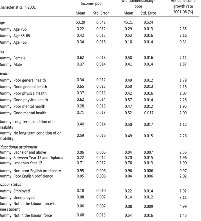
Understanding the growth gap between the two groups of poor is important for various reasons. First, it will help us to understand why poverty de…nitions di¤er as regards their capacity to identify those individuals who are less likely to participate and bene…t from economic growth. Most importantly, understanding the di¤erences between the multidimensional and the income-poverty measures is crucial to determine the non-income dimensions that are key for identifying low-growth groups and that are therefore expected to have a critical role in shaping pro-poor growth evaluations. Table 4 presents the characteristics of the poor in 2001 as well as the average annual growth rates experienced by speci…c demographic groups between 2001 and 2008. We …nd that those identi…ed as poor according the multidimensional poverty index in 2001 are on average more than 7 years younger than those in the income-poor group. Remarkably, despite of being a younger population, the multidimensionally-poor have worse health conditions than low-income people. Thus, the incidence of people with poor general, physical, and mental health is respectively about 15, 5, and 19 percentage points larger among those who are poor in multiple dimensions. Also, the proportion of individuals that report some type of disability or long-term health condition in this group is 10 percentage points larger than in the income-poor group. Those who are identi…ed as poor by the multidimensional poverty index have lower educational attainment than those who were on low-income: the
incidence of individuals with less than Year 12 among the income-poor is about …ve points lower than among those who are poor in multiple dimensions (71 versus 76 per cent).
As the …gures on income growth rates in the right column of Table 4 show, people with poor health, disabilities, and lower educational attainment experienced little income growth compared to other groups. The higher prevalence of these individuals among the multidimensionally-poor could therefore account for the growth gap of this group. To check the validity of this hypothesis we will make use of conterfactual analysis. In particu-lar, we follow the Oaxaca-Blinder and DiNardo-Fortin-Lemieux approaches to investigate the role of observed characteristics in explaining di¤erences in the distribution of income gains between the multidimensionally and the income-poor. Let GM P and GIP denote
the groups with the poorest 15th per cent as de…ned by the multidimensional and the income poverty indices in 2001, respectively. Let FM P(g) and FIP(g) be the distribution
of growth rates (or absolute variations) among these groups. The well-know regression based approach …rst proposed by Oaxaca (1973) and Blinder (1973) allows us to decom-pose di¤erences in mean growth rates observed between the two groups of poor people. For each individuali we assume that the income growth rate follows the model
gi =xi +ei;
wherexiis a1xkvector of covariates, is the vector of parameters, andeiis the error term
satisfyingE(eijxi) = 0:LetbM P andbIP be OLS estimates of derived using observations
from the GM P and GIP groups. Let xIPbM P denote the counterfactual value of the
mean growth rate among the multidimensionally-poor if those were given the observed characteristics of the income-poor. Then, the di¤erence between the mean growth rate of the of the multidimensionally-poor,gM P, and the average growth rate of the income-poor, gIP, can be expressed as
gIP gM P =xIP(bIP bM P) + (xIP xM P)bM P;
where the …rst term on the right-hand side captures the part of the gap caused by dif-ferences in coe¢ cients, while the second term measures the expected change in the mean growth rate due to the shift in observed characteristics between the two groups (explained
e¤ect).
In contrast to the Oaxaca-Blinder decomposition, the DiNardo, Fortin, and Lemieux (1996)-DFL thereafter- reweighting approach permits evaluation of the contribution of co-variates to di¤erentials across the whole distribution instead of focusing only on the mean. Each individual observation is drawn from a common joint density function f(g; x; G),
Table 4.Characterization of the initially poor
Characteristics in 2001 Income- poor
Multidimensionally-poor Annual incomegrowth rate 2001-08 (%) Mean Std. Error Mean Std. Error
Age 53.20 0.542 45.21 0.524 Dummy: Age <35 0.22 0.012 0.29 0.013 2.35 Dummy: Age 35-65 0.42 0.013 0.53 0.016 2.16 Dummy: Age >65 0.34 0.015 0.16 0.014 0.31 Sex Dummy: Female 0.62 0.013 0.58 0.016 2.11 Dummy: Male 0.37 0.014 0.41 0.014 1.87 Health
Dummy: Poor general health 0.34 0.012 0.49 0.012 1.79
Dummy: Good general health 0.65 0.013 0.50 0.013 2.15
Dummy: Poor physical health 0.37 0.013 0.42 0.016 1.07
Dummy: Good physical health 0.62 0.014 0.57 0.014 2.28
Dummy: Poor mental health 0.28 0.013 0.47 0.012 1.95
Dummy: Good mental health 0.71 0.013 0.52 0.017 2.09
Dummy: Long-term condition of or
disability 0.40 0.014 0.50 0.017 1.12
Dummy: No long-term condition of or
disability 0.59 0.016 0.49 0.015 2.26
Educational attainment
Dummy: Bachelor and above 0.06 0.006 0.04 0.007 2.55
Dummy: Between Year 12 and Diploma 0.22 0.012 0.20 0.015 1.96
Dummy: Less than Year 12 0.71 0.012 0.76 0.013 1.90
Dummy: Non-poor English proficiency 0.95 0.006 0.96 0.006 0.97
Dummy: Poor English proficiency 0.05 0.006 0.04 0.006 2.02
Labour status
Dummy: Employed 0.18 0.010 0.22 0.014 1.92
Dummy: Unemployed 0.08 0.007 0.14 0.012 3.11
Dummy: Not in the labour force-full
time student 0.06 0.007 0.08 0.009 4.99
Dummy: Not in the labour force 0.68 0.013 0.54 0.016 1.45
Notes: Income-poor and multimensionally-poor groups defined using the 15thpercentile of each poverty index in 2001 as poverty threshold. For the definition of the categories, see Table A1 in the appendix. Average annual growth rates for the different categories computed using all the observation in the panel. All estimates computed using longitudinal responding person weights.
whereg, x;and Grefer to income growth rate, observed characteristics, and group mem-bership, respectively. The marginal distribution of growth rates for group GM P is then
given by
fGM P(g) =
Z
x
f(gjx; GM P) fx(xjGM P)dx;
where x is the domain of individual attributes and fx(xjGM P) =
Z
g
f(g; xjGM P)dg;
with g being the domain of annual growth rates. The counterfactual distribution for
group GM P is de…ned as the distribution of income gains that would prevail assuming
groupGM P had the same observed characteristics of groupGIP. Following DFL, this can
be expressed as fGIP GM P(g) = Z x f(gjx; GM P) fx(xjGIP)dx= Z x f(gjx; GM P) x(x)fx(xjGM P)dx;
where x(x) is the ‘reweighting’function given by
x(x) = fx(xjGIP) fx(xjGM P) = P(G=GM P) P(G=GIP) P(G=GIPjx) P(G=GM Pjx) ;
where the last equality holds from Bayes’rule. The …rst ratio is just the relative frequency of each group, which is constant and can therefore be ignored for the reweighting process. For the second term, following DFL, we estimate a probit model for the probability of belonging to each groupGIP andGM P;given characteristicsx. The counterfactual
distri-bution functionFGIP
GM P(g)can then be used to decompose the di¤erences in the distribution
of income gains between both groups as follows
FIP(g) FM P(g) = [FIP(g) FGGM PIP (g)] + [F
GIP
GM P(g) FM P(g)]:
The second term of the equation represents theexplained part of the gap which can be attributed to di¤erences in the distribution of observed characteristics between the two groups. In contrast to the Oaxaca-Blinder approach, this decomposition can be used to
evaluate the contribution of covariates to explain di¤erences across the whole distribution. Thus, the di¤erential at any percentile p can be decomposed as
pIP(g) pM P(g) = [pIP(g) pGIP
GM P(g)] + [p
GIP
GM P(g) pM P(g)]:
To determine to contribution of each covariate (or set of covariates) to explain the overall gap we apply a Shapley-type decomposition procedure (see Shorrocks 1999 and Sastre and Trannoy 2002). Widely used in inequality decomposition analysis, this decom-position identi…es the contribution of each factor with the expected marginal e¤ect on the explained gap of eliminating the covariate when computing the conterfactual estimates. LetK = (1; :::; j; :::; k)be the set of covariates, and letS K denote any possible subset of covariates. The Shapley contribution of characteristic j is given by
Shj = P S K; j2S (s 1)!(k 1)! k! [e(S) e(Snfjg)] e(K) with k X j=1 Shj = 1
where s is the size of the subset, and e( ) is the explained e¤ect that depends on the particular set of covariates used to derive the counterfactual estimate.18
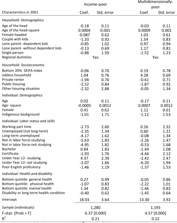
The OLS and the probit regressions used for the counterfactual analysis include, as explanatory variables, multiple socioeconomic variables that are expected to in‡uence in-dividuals’ ability to bene…t from economic growth.19 We group the covariates into …ve categories. The …rst one includes demographic information about the household where the individual lived in 2001, including the age and sex of the head; type of family ex-pressed with dummy variables for couples with kids, couples with no children, lone-parent households with and without dependent children, singles, and other family types; and thirteen dummy variables for the major statistical regions reported in HILDA.20 Details 18For both the Oaxaca-Blinder and the DFL regression decompositions,e(S)is obtained setting all the
other coe¢ cients but those of the covariates inS equal to zero.
19Notice the aim of this analysis is to evaluate the contribution of the di¤erences in the distribution
of observed characteristics between the two poor groups to explain the growth gap. The econometric speci…cations are simply thought to identify the statistical association between individuals’characteristics and bene…ts from growth. Issues of endogeneity and selection bias were not addressed which implies that no causal relationship can be assessed from our results.
20These are Sydney, other regions of New South Wales, Melbourne, other areas of Victoria, Brisbane,
rest of Queensland, Adelaide, other regions of South Australia, Perth, rest of Western Australia, Tasma-nia, Northern Territory, and Australian Capital Territory.
on the initial socioeconomic conditions of the household are considered in a separate cat-egory. We include an indicator variable to identify those individuals living in an area which falls into the lowest 20 per cent most disadvantaged areas in Australia as measured by the index of relative socioeconomic disadvantage for areas (SEIFA); type of housing tenure with dummy variables for owners, renters, and rent-free households; and a dummy variable to indicate whether the individual belongs to a jobless household. Demographic characteristics of individuals in 2001 including age, sex, and an indicator variable identi-fying those with indigenous backgrounds are grouped in a third category. Information on individuals’initial labour statuses, educational attainment, and English skills are consid-ered in a separate group. This includes dummies for people working part-time, full-time, unemployed, long-term unemployed, full-time students, and other individuals out of the labour force; indicator variables for those with graduate or postgraduate education, bach-elor or advanced diploma, certi…cate I, II, III or IV, Year 12 or less but still engaged in education,and those with Year 12 or less who were not in education; and a dummy variable taking value one for those who speak a language other than English at home and report that they do not speak English well or does not speak English at all. Lastly, the health category includes details on disabilities and the general, physical, and mental health status of the individual. In particular, for the three health dimensions we de…ne …ve dummies, one for each of the …ve quintiles of the corresponding health index reported in HILDA.21 The presence of disabilities is captured by an indicator variable that
acti-vates when the individual reports a long-term health condition or disability that restricts everyday activities for at least six months. The results of the regressions used for the analysis are presented in the Appendix.22
Table 5 shows the results of the counterfactual analysis for the case of the annual growth rates. Results for annual variations are quite similar and yield similar conclusions, so they are not discussed here for the sake of brevity. It is clear from this table that di¤erences in observed characteristics contribute to explain why those who were poor according to multidimensional index bene…ted less from growth than those in low-income. Thus, for the mean, results from the Oaxaca-Blinder decomposition suggest that the
21The general, physical, and mental health indices take values between 0 and 100 and are based on the
SF-36 Health Survey included in HILDA.
22The results of the multiple regressions run to evaluate the contribution of each group of characteristics
Table 5.Oaxaca-Blinder and DiNardo-Fortin-Lemieux counterfactual decompositions Annual income growth rate, 2001-2008
Income-poor (%) Multidimensionally-poor (%) Raw gap poor counterfactual (%)Multidimensionally- Explainedgap Oaxaca-Blinder Mean 5.91 2.81 3.10 3.63 0.82 (0.375) (0.163) (0 .520) (0.618) (0.052) DiNardo-Fortin-Lemieux Mean 5.91 2.81 3.10 3.25 0.45 (0.375) (0.163) (0 .520) (0.312) (0.118) Percentile: 10th -1.81 -6.31 4.57 -3.77 2.54 (0.072) (0.535) (0.820) (0.293) (0.332) 20th 0.06 -2.82 2.88 -1.09 1.73 (0.251) (0.934) (0.403) (0.362) (0.498) 50th 3.32 2.06 1.26 1.90 -0.15 (0.177) (0.183) (0.237) (0.534) (0.439) 80th 11.05 8.60 2.45 7.52 -1.08 (0.401) (0.562) (0.298) (0.626) (0.496)
Shapley contributions of observed characteristics to the explained gap in mean growth rates
Oaxaca-Blinder DiNardo-Fortin-Lemieux
Group of covariates Marginal
effect Shapley value (%) Marginal effect Shapley value (%) Household: demographics 0.04 4.87 0.05 11.11 (0.198) (5.00) (0.08) (28.81) Household: socioeconomic 0.19 23.17 0.16 35.55 (0.141) (4.55) (0.09) (13.95) Individual: demographics -0.15 -18.29 -0.20 -44.44 (0.078) (4.59) ( 0.151) (12.71)
Individual: labour status and skills -0.06 -7.31 -0.05 -11.11
(0.365) (6.38) (0.135) (52.81)
Individual: health and disability 0.80 97.56 0.49 108.89
(0.340) (5.94) (0.176) (20.22)
Total 0.82 100.00 0.45 100.00
Notes: Income and multimensionally-poor groups defined using poverty thresholds equal to the 15thpercentile of each poverty index in 2001. For a description of the groups of covariates considered to estimate the Shapley contribution see the main text. Standard errors in parentheses derived using bootstrap with 1,000 replications. All estimates computed using longitudinal responding person weights.
average growth rate of the multidimensionally-poor would increase about 30 per cent (from 2.81 to 3.63) if the distribution of characteristics of the income-poor was assumed.23 This implies that di¤erences in characteristics account for more than one quarter of the gap in mean growth rates. Figures from the DFL decomposition indicate that the e¤ect of characteristics is not uniform over the whole distribution. Counterfactual estimates for the 10th and 20th percentiles show that the contribution of characteristics is particularly large at the bottom of the distribution, where di¤erences in characteristics account for more than 50 per cent of the gap between the two sets of poor people. In contrast, we …nd that characteristics cannot explain the observed gap in the middle and upper parts of the distribution. Indeed, the gap at the median and the 80th percentile increases when compositional di¤erences are taken into account. The Shapley contributions of each group of covariates to the explained gap in mean are presented in the bottom part of the table. Interestingly, both the Oaxaca-Blinder and DFL methodologies point to di¤erences in health conditions and the incidence of disability as the most explicative factor for the gap between the multidimensionally and the income-poor. Thus, di¤erences in the distribution of health and the larger incidence of people with disabilities or long-term health condition among those who were poor in multiple dimensions jointly account for 98-108 per cent of the explained di¤erence between the average growth rate of this group and that of the income-poor. The initial socioeconomic conditions of the household is the second most important factor with a contribution that is between 23 and 35 per cent, depending on the decomposition method adopted. The Shapley value of the demographic characteristics of individuals is negative, which means that the gap in mean growth rates between the two groups widens once di¤erences in age, sex, and indigenous background are controlled for. This could be explained by the larger prevalence of individuals above 65 years of age who had little income growth among the income-poor relative to the multidimensionally-poor (see Table 4).24 Finally, the Shapley contribution of the initial labour status and skills is also negative but statistically insigni…cant. In this case, from the …gures in Table 4 we know that the income-poor population has higher educational attainment than those who 23Note this conterfactual exercise provides an estimate of the income gains of the
multidimensionally-poor assuming the characteristics of the income-multidimensionally-poor. This implies that di¤erences in returns between these two groups are weighthed by the characteristics of the income-poor. To check the robustness of the results we also estimated the alternative decomposition which weights di¤erences in returns by the characteristics of the multidimensionally-poor. The results of this exercise, available upon request, are consistent with the ones presented here.
24The incidence of people with indigenous background is slightly higher among the
were poor in multiple dimensions. However, this e¤ect could be more than o¤set by the larger prevalence among the income-poor of individuals who were out of the labour force and bene…ted relatively little from growth.
Conclusions
In …rst decade of the XXI century Australia consolidated its position as a high-growth economy in the developed world. In the period 2000-2009, Australia experienced one of the largest output growth rates among OECD, only overtaken by a group of countries with lower initial income including Turkey, Hungary, Greece, the Czech Republic, Korea, Poland, and the Slovak Republic. Recent evidence suggests, however, that the bene…ts from growth in Australia were not evenly distributed. In the last decade Australia wit-nessed an increase in income inequality and the share of income held by those at the top of the income distribution (ABS, 2011). These results are consistent with the up-ward trend in income di¤erences and relative income poverty documented earlier in the literature (Wilkins 2007, Saunders and Hill 2008). To date much has been written about the Australian economic miracle, however, yet little is known on the extent to which the strong economic growth has been pro-poor or not. Our aim in this paper was to …ll this gap.
Pro-poor growth analysis contributes to our understanding of the distributional ef-fects of growth by providing insights that cannot be derived from the analysis of standard inequality and poverty measures. Thus, while inequality and poverty measures are con-cerned with the di¤erences in the income distribution and the income gap of those who are below some threshold, respectively, pro-poor growth measures evaluate the impact of growth on poverty reduction by looking at the extent to which growth bene…ts the poor. In this paper we have investigated the pro-poorness of Australian growth using anony-mous and non-anonyanony-mous pro-poor growth measures. These two approaches complement each other in that they focus on di¤erent aspects of the distributional change associated to economic growth. Growth assessments consistent with the anonymity axiom evaluate the distributional impact of growth looking only at the income change experienced by the bottom positions of the income parade without taking into account whether these positions are occupied by the same individuals or not. In contrast, non-anonymous eval-uations focus on the mobility aspect of growth looking exclusively at the income change experimented by those who were initially poor. An important issue that arises in this type of evaluation is how to identify those initially in poverty. We compare the results based
on the standard income-poverty with those derived using a multidimensional de…nition of poverty that embraces multiple non-income attributes.
Results for the anonymous measures suggest that Australian growth in the last decade was pro-poor only according to the poverty reducing de…nition of pro-poorness. This is the weakest concept of pro-poor growth as it identi…es as pro-poor every growth pattern that increases the income of the poor, regardless of how the bene…ts from growth are distributed among the di¤erent positions in the income distribution. However, the growth incidence curves based on HILDA data show that Australia’s growth between 2001 and 2008 was highly concentrated at the top of the income distribution. In fact, while the bottom positions were the ones that experienced the lowest income gain, the only positions that grew more than the mean were those above the 90th percentile. As a consequence, Australia’s growth in the last decade was not pro-poor according to any concept that implies a particular bias of growth in favor of the poor.
We exploit the longitudinal information in HILDA to study the e¤ect of growth on those who were initially poor. Our results based on non-anonymous measures indicate that the pro-poorness of growth in this case critically depends on the de…nition of poverty considered. Thus, while there exists high income mobility, with those initially in the low-income group growing more than those with high incomes, the income gain of those identi…ed as poor according to the multidimensional poverty measure was far below that of the mean. Therefore, we can conclude that growth was more income-poor than pro-multidimensionally poor. We use counterfactual analysis to assess the extent to which this result is due to di¤erences in the distribution of demographic and socioeconomic characteristics between the two groups of poor. Interestingly, we …nd that di¤erences in the distribution of health and the larger incidence of people with disabilities or long-term health condition among those who were poor in multiple dimensions explain why growth was less pro-multidimensionally poor. Indeed, the average annual growth rate of those who were poor according to the multidimensional measure would increase about 16-30 per cent if the health distribution of the income-poor was assumed. This highlights the sensitivity of non-anonymous growth evaluations to the way poverty is de…ned, in particular, to whether the de…nition of the poor incorporates information about the health dimension of well-being or not.
References
[1] Araar A. and Duclos, J. Y. (2007). “DASP: Stata modules for distributive analysis,” Statistical Software Components S456872, Boston College Department of Economics. [2] Atkinson, A.B. (1987). “On the Measurement of Poverty,”Econometrica, Vol. 55,
pp. 749–764.
[3] Australian Bureau of Statistics (2006) Socio-Economic Indexes for Areas (SEIFA) -Technical Paper, 2006, cat. 2039.0.55.001, ABS Canberra.
[4] Australian Bureau of Statistics 2011, Household Income and Income Distribution, cat. no. 6523.0, ABS, Canberra.
[5] Azpitarte, F (2012). “Has Economic Growth in Australia Been Pro-Poor?”forthcom-ing in P. Smyth (ed), Inclusive Growth: an Australian Approach, Allen & Unwin, NSW.
[6] Blinder, A. S. (1973). “Wage Discrimination: Reduced Form and Structural Esti-mates,”Journal of Human Resources, Vol. 8, No. 4, pp. 436–455.
[7] Bourguignon, F. (2010). “Non-anonymous Growth Incidence Curves, Income Mobil-ity and Social Welfare Dominance,”Journal of Economic Inequality, Vol. 9, No. 4, pp. 605-627.
[8] Buhmann, B., Rainwater, L., Schmaus G., and Smeeding, T. J. (1988). “Equivalence Scales, Well-Being, Inequality, and Poverty: Sensitivity Estimates Across Ten Coun-tries using the Luxembourg Income Study (LIS) Database,”Review of Income and Wealth, Vol. 34, pp. 115–142.
[9] Datt, G. and Ravallion, M. (1992). “Growth and Redistribution Components of Changes in Poverty Measures: A Decomposition with Applications to Brazil and India in the 1980s,”Journal of Development Economics, Vol. 38, pp. 275-295. [10] Deutsch, J. and Silber, J. (2011). “On Various Ways of Measuring Pro-Poor
Growth,”Economics: The Open-Access, Open-Assessment E-Journal, Vol. 5, 2011-13. http://dx.doi.org/10.5018/economics-ejournal.ja.2011-2011-13.
[11] DiNardo, J., Fortin, N., and Lemieux, T. (1996). “Labor market institutions and the distribution of wages, 1973-1992: A semiparametric approach,”Econometrica Vol. 64, pp. 1001-1044.
[12] Duclos, J.-Y (2009). “What is pro-poor?”Social Choice and Welfare, Vol.32, No.1, pp. 37-58.
[13] Essama-Nssah, B. and Lambert, P. J. (2009). “Measuring Pro-Poorness: a Unifying Approach
[14] with New Results,”Review of Income and Wealth, Vol. 55, pp. 752-778.
[15] Foster J. (1985). “Inequality Measurement” In: Peyton Young H (ed.), Fair Alloca-tion, American Mathematical Society. Proceedings of Simposia in Applied Mathe-matics Vol. 33, pp. 31-68.
[16] Foster, J. and Shorrocks, A.F. (1988). “Poverty orderings,”Econometrica, Vol. 56, pp. 173–177.
[17] Foster, J., Greer J., and Thorbecke, E. (1988). “A Class of Decomposable Poverty Measures,”Econometrica Vol. 52, p.p. 761-765.
[18] Grimm, M. (2007). “Removing the Anonymity Axiom in Assessing Pro-Poor Growth,”Journal of Economic Inequality, Vol. 5, No. 2, pp. 179-197.
[19] Kakwani, N (1993). “Poverty and Economic Growth with Application to Cote D’Ivoire,”Review of Income and Wealth, Vol. 39, No.2, pp. 121-139.
[20] Kakwani, N. and Pernia, N. (2000). “What is Pro-Poor Growth,”Asian Development Review, Vol. 16, No. 1, pp. 1–22.
[21] Kakwani, N. and Son, H. (2008). “Poverty Equivalent Growth Rate,”Review of Income and Wealth, Vol. 54, No. 4, pp. 643-655.
[22] Klasen S. (2008). “Economic Growth and Poverty Reduction: Measurement Issues using Income and Non-Income Indicators,”World Development, Vol. 36, No. 3, pp. 420-445.
[23] Osmani, S. (2005). De…ning pro-poor growth. One Pager, 9. Brazilia: UNDP Inter-national Poverty Centre.
[24] Oaxaca, R. L. (1973). “Male-female Wage Di¤erentials in Urban Labor Markets,”
International Economic Review, Vol. 14, No. 3, pp. 693–709.
[25] Ravallion, M. and Chen, S. (2003). “Measuring Pro-Poor Growth,”Economics Let-ters, Vol. 78, pp. 93–99.
[26] Saunders, P. and Bradbury, B. (2006). “Monitoring Trends in Poverty and Income Distribution: Data, Methodology, and Measurement,”The Economic Record, Vol. 82, no. 258, pp. 341-364.
[27] Saunders, P. and Hill,T. (2008). “A Consistent Poverty Approach to Assessing the Sensitivity of Income Poverty Measures and Trends,”The Australian Economic Re-view, Vol. 41, no. 4, pp. 371-88.
[28] Scutella, R., Horn, M., and Wilkins, R. (2009a). "Measuring Poverty and Social Exclusion in Australia: A Proposed Multidimensional Framework for Identifying Socio-Economic Disadvantage,” Melbourne Institute Working Paper No. 4/09. [29] Scutella, R., Kostenko, W., and Wilkins, R., (2009b). “Estimates of Poverty and
Social Exclusion in Australia: A Multidimensional Approach,” Melbourne Institute Working Paper No. 26/09.
[30] Stiglitz, J. E., Sen A., and Firoussi, J.P. (2009). Report by the Commission on the Measurement of Economic Performance and Social Progress. (available at http://www.stiglitz-sen…toussi.fr/en/index.htm).
[31] Son, H. (2004). “A note on pro-poor growth,”Economic Letters, Vol. 82, pp. 307.314. [32] Ware, J.E., Snow, K.K., Kosinski, M., and Gandek, B. (2000), SF-36 Health Survey:
Manual and Interpretation Guide, QualityMetric Inc., Lincoln, RI.
[33] Watts, H., (1968). An economic de…nition of poverty, in: D.P. Moynihan, ed., On understanding poverty (Basic Books,New York).
[34] Wilkins, R. (2007), “The Changing Socio-Demographic Composition of Poverty in Australia: 1982-2004,”Australian Journal of Social Issues, Vol. 42, no. 4, pp. 481-501.
[35] Wooden, M and Watson, N. (2007). “The HILDA Survey and its Contribution to Economic and Social Research (So Far),”Economic Record, Vol.83, No.261, pp. 208-231.
Appendix
4.4
The index of multidimensional poverty
The poverty index proposed in Scutella et al. (2009a,2009b) combines information on twenty-one indicators from seven di¤erent domains: material resources; employment; ed-ucation and skills; health and disability; social; community; and personal safety. Table A.1 presents a description of the indicators included in each domain. For any individuali the measure of social exclusion,xS
i , is de…ned as seven minus the weighted sum of the level
of social exclusion experienced within each domain, xid, where every domain is assigned
equal weight: xSi = 7 7 X d=1 xid:
The level of exclusion in any domain is given by the actual proportion of indicators within the domain in which the individual is deprived, which can expressed as follows
xid= PKd k=1x k id Kd ; where xk
idis a binary indicator taking value 1 when the individual is deprived in the
indicatorkof social exclusion included in the domaind, andKdrefers to the total number