Metrics for sampling-based motion planning

(1)

A Dissertation by

MARCO ANTONIO MORALES AGUIRRE

Submitted to the Office of Graduate Studies of Texas A&M University

in partial fulfillment of the requirements for the degree of DOCTOR OF PHILOSOPHY

December 2007

(2)

A Dissertation by

MARCO ANTONIO MORALES AGUIRRE

Submitted to the Office of Graduate Studies of Texas A&M University

in partial fulfillment of the requirements for the degree of DOCTOR OF PHILOSOPHY

Approved by:

Chair of Committee, Nancy M. Amato

Committee Members, Ricardo Guti´errez-Osuna Donald H. House

John Keyser Head of Department, Valerie E. Taylor

December 2007

(3)

ABSTRACT

Metrics for Sampling-Based Motion Planning. (December 2007)

Marco Antonio Morales Aguirre, B.S., Universidad Nacional Autónoma de México; M.S., Universidad Nacional Autónoma de México

Chair of Advisory Committee: Dr. Nancy M. Amato

A motion planner finds a sequence of potential motions for a robot to transit from an initial to a goal state. To deal with the intractability of this problem, a class of methods known as sampling-based planners build approximate representations of potential motions through random sampling. This selective random exploration of the space has produced many remarkable results, including solving many previously unsolved problems. Sampling-based planners usually represent the motions as a graph (e.g., the Probabilistic Roadmap Methods orPRMs), or as a tree (e.g., the Rapidly exploring Random Tree or RRT). Although many sampling-based planners have been proposed, we do not know how to select among them because their different sampling biases make their performance depend on the features of the planning space. More-over, since a single problem can contain regions with vastly different features, there may not exist a simple exploration strategy that will perform well in every region. Unfortunately, we lack quantitative tools to analyze problem features and planners performance that would enable us to match planners to problems.

We introduce novel metrics for the analysis of problem features and planner performance at multiple levels: node level, global level, and region level. At the node level, we evaluate how new samples improve coverage and connectivity of the evolving model. At the global level, we evaluate how new samples improve the structure of the model. At the region level, we identify groups or regions that share similar features. This is a set of general metrics that can be applied in both graph-based and tree-based

(4)

planners. We show several applications for these tools to compare planners, to decide whether to stop planning or to switch strategies, and to adjust sampling in different regions of the problem.

(5)

To my wife Aim´ee, blessing love and fortitude:

tonehuan ticeixtli ticeyollotl (you and me, one face, one heart)

To my parents Marcos and Esperanza:

(6)

ACKNOWLEDGMENTS

I would like to thank Dr. Nancy Amato. She is a great mentor and research leader. Her guidance was key to find the right way in this journey countless times. It has been a privilege and joy to be part of her research group.

Thanks to Dr. Ricardo Guti´errez-Osuna, Dr. Donald House, and Dr. John Keyser, for their comments that enriched this research and for their support. Also, thanks to the many professors I met at A&M, for their classes, talks, and discussions.

Thanks to the members of the Parasol Lab for their great work that supports our research, for the many discussions, and for the rewarding collaborations, especially: Burchan Bayazit, Jyh-Ming Lien, Olga Pearce, Roger Pearce, Samuel Rodr´ıguez, Guang Song, Xinyu Tang, Lydia Tapia, Shawna Thomas, Aim´ee Vargas, and Dawen Xie. Also, thanks to the great students I could meet at A&M.

Thanks to the Comission M´exico-United States for Educational and Cultural Ex-change for the Fulbright-Garcia Robles Scholarship that allowed me to pursue a PhD. Also, thanks to the Mexican Government and its Consejo Nacional de Ciencia y Tec-nolog´ıa , and to the U.S. Government, its Department of State, and the Institute of International Education.

Thanks to Marcos and Esperanza, my parents. They showed me how to search for my way in life, they carefully nurtured my curiosity, they let me go, and they have always been there for me. Also, thanks to Roc´ıo, my sister, for her encouragement and friendship.

My most wholehearted thanks to Aim´ee, my loved wife and comrade. Her courage fed my enthusiasm to embark in this adventure. Her support has kept me afloat when my strength has dwindled. Her tenderness has warmed my heart in the worst times. Her smile is the tastiest delicacy. We are truly one face and one heart.

(7)

IV EVALUATION STRATEGY . . . 23

A. Planners . . . 23

B. Motion Planning Problems . . . 25

C. Experimental Setup . . . 28

V NODE-LEVEL METRICS . . . 32

A. Type and Amount of Improvement Produced by a New Node 32 B. Population Distribution of Node Types . . . 40

(8)

CHAPTER Page

D. Overhead of Node-Level Metrics . . . 45

VI GLOBAL-LEVEL METRICS . . . 47

A. Changes in Motion Pathways Produced by New Nodes . . 47

B. Detection of Relative Change of Global-Level Metrics . . . 53

C. Overhead of Global-Level Metrics . . . 55

VII REGION-LEVEL METRICS . . . 58

A. Region Construction . . . 58 1. Features . . . 59 2. Clustering Strategies . . . 59 a. Axis-Aligned Regions . . . 59 b. Simple-Feature Regions . . . 60 c. Coverage Regions . . . 61

3. Frequency of Region Updates . . . 63

4. Region Statistics . . . 63

B. Overhead of Region-Level Metrics . . . 64

VIII APPLICATIONS AND EXPERIMENTS . . . 66

A. Learning Process of Planners . . . 66

1. Evolution of the Node-Level Metrics . . . 66

2. Evolution of the Global-Level Metrics . . . 69

B. Stages of the Learning Process of Planners . . . 76

1. How Stage Transitions Can Be Detected? . . . 80

2. What Can Be Done WhenLearning Decay Starts? . . 83

C. Distribution of Nodes in the C-Space . . . 85

1. What Is the Population Distribution of Regions for Different Planners? . . . 85

2. How Effective Are Planners in Biasing towards Highly-Constrained Regions? . . . 90

3. How Do Coverage Regions Evolve in Incremental Planners? . . . 90

4. How Can We Adapt Planning Based on Region Complexity? . . . 92

D. Comparison of Metrics at the Start of Learning Decay for Different Roadmap-Based Planners . . . 94

E. Metrics in High-DOF Problems . . . 97

(9)

CHAPTER Page REFERENCES . . . 106 VITA . . . 114

(10)

LIST OF TABLES

TABLE Page

I Visibility of Growth Sites in serial-hook-5 . . . 44

II Node-Level Metrics Overhead inrigid-maze . . . 46

III Basic-PRM onrigid-windows. Robot Width = 1 . . . 51

IV Global-Level Metrics Overhead in rigid-maze . . . 57

V Region-Level Metrics Overhead inrigid-maze . . . 65

VI Population Distribution of Nodes in rigid-maze. Deviation . . . 71

VII Population Distribution of Nodes in rigid-walls. Deviation . . . 71

VIII Population Distribution of Visibility Regions inrigid-maze. Deviation 88 IX Population Distribution of Visibility Regions inrigid-walls. Deviation 90 X Number of Samples Needed for Planners to Get to Goal Region . . . 92

XI Planners at Start of Learning Decay on rigid-maze . . . 95

XII Planners at Start of Learning Decay on rigid-hook . . . 97

(11)

LIST OF FIGURES

FIGURE Page

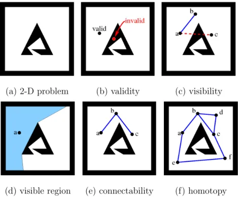
1 Validity, visibility, visible region, connectability, and homotopy in (a) the C-Space of a point robot moving in the plane. (b) A valid configuration inF and an invalid configuration inO. (c) Visibility with straight-line local planner: a can see b but it can not see c. (d) The visible region for a, with straight-line local planner, in light blue. (e) a and c are connectable (τ(a, c) = {a, b, c}). (f) Two homotopy classes between a and c: τ1 = {a, b, c} and τ2 ={a, b, d, c} can be continuously transformed into each other;

2. τ3 ={a, e, f, c}cannot be transformed into τ1 nor τ2. . . 7 2 Witness queries between “witness” configurations 1 and 2. (a)

Only witness 1 is connected to the model, there has not been found any path between witnesses. (b) Both witnesses are con-nected to the model, one path between them has been found. (c) Both witnesses are connected to the model, two paths between them have been found. The witness evaluation does not make a distinction between case (b), with only one pathway between

witnesses, and case (c), with two pathways between witnesses. . . 17 3 Problem: rigid-maze. (a) solid view. (b) wire-view shows the

internal tunnels. (c) close-up view of the robot. . . 26 4 Problem: rigid-windows. The robot has 3 translational degrees of

freedom. Four pathways of different sizes allow the robot to cross from the front to the back. The start and goal configurations are

at each side of the leftmost wall. . . 26 5 Problem: rigid-hook. In order to get through the passages, the

6-DOF robot needs to perform translations and rotations. . . 27 6 Problem: rigid-walls. Incremental planners find their in

(12)

FIGURE Page 7 Problem: serial-hook-5. The 10-DOF robot can fold and unfold

to get through the opening that divides the environment. This is

a variation of therigid-hook problem.. . . 29 8 Problem: serial-spring-98. The 103-DOF robot folds and unfolds

to get above the wall that divides the environment. . . 29 9 Classification of new nodes when modeling the C-Space of a point

robot moving in the plane shown in (a). (b) The first sample in the model with its visibility region. (c) A new sample lying outside the visibility region of any other sample creates another component with its own visibility region. (d) A new sample lying in the overlap of the visibility region of two components allows to merge them. (e) A new sample lying inside the visibility region of one component expanding its visibility: cc-expand. (f) A new sample lying inside the visibility region of one component without

changing its visibility: cc-oversample. . . 33 10 An implementation of classification of new nodes. (a) State of M

before a new node is added. (b) New node increases the number of components: cc-create. (c) New node reduces the number of components: cc-merge. (d) New node v cannot connect to any neighbor ofv0: cc-expand. (e) New nodev cannot connect to 50% of the neighbors of v0: cc-expand for Et = 0.5. (f) New node v

can connect to all the neighbors of v0: cc-oversample. . . 35 11 Absolute error in the classification ofcc-expand nodes for different

approximations (p = 0.0 no additional connection test, p = 0.1, and p= 0.5) with respect to a full test (p= 1.0) vs. nodes in the model for roadmap-based planners applied to therigid-maze prob-lem. (a)Gauss-PRM. (b)OBPRM. Each line represents statistics from four different runs with standard deviations are below 5% be-fore 1000 nodes in all the experiments. Basic-PRM andMAPRM are similar toGauss-PRM, andBridge-Test is similar toOBPRM.

(13)

FIGURE Page 12 Absolute error in the classification ofcc-expand nodes for different

approximations (p = 0.0 no additional connection test, p = 0.1, and p= 0.5) with respect to a full test (p= 1.0) vs. nodes in the model for incremental planners applied to therigid-mazeproblem. (a) RPP. (b) RRT-Expand. Each line represents statistics from four different runs with standard deviations are below 5% before 1000 nodes in all the experiments. EST shows error amounts in betweenRPP and RRT-Expand, and RRT-Connect is similar to

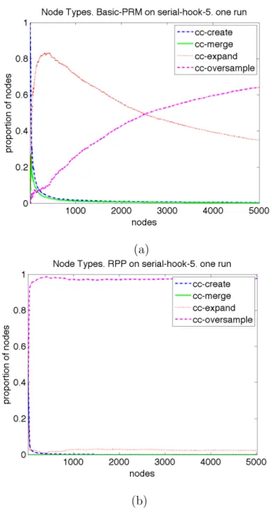
RRT-Expand. Overheads are shown in Table II.. . . 39 13 Population distribution of node types produced by individual

in-stances of planners when modeling theserial-hook-5 problem. (a)

Basic-PRM. (b) RPP. . . 41 14 Population distribution of node types produced by eight instances

ofBasic-PRM when modeling theserial-hook-5 problem. (a) Av-erage populations with nodes in logarithmic scale to better see evolution in initial iterations. (b) Standard deviation of popula-tions with both nodes and proportion of nodes shown in logarith-mic scale, the standard deviations for all node types fall below

10% before 50 nodes. . . 42 15 Visibility ratio of growth sitesa,c, and eas they are added to the

model and connected with a bidirectional local planner. (a) new nodeais added, Va= 2/3. (b) new node cis addedVc= 0/3, the visibility of a needs to be updated Va = 2/4. (c) new node e is

addedVe= 3/3, the visibility of a needs to be updated Va = 3/5. . . 44 16 Global changes in model topology resulting from new nodes and

connections. (a) State of M before adding new nodes, in the C-Space there is one component and two homotopy classes, or distinct pathways, between a and b; in contrast, the model has three components and no pathway betweena andb. (b) Two new nodes and their connections improve the topology of the model to have one component and one homotopy class between a and b. (c) one more node and its connections improve the topology of the model to have one component and two homotopy classes

(14)

FIGURE Page 17 Evolution of global-level metrics for one instance of Basic-PRM

on the rigid-windows problem. (a) Number of components. (b) sum-diameter andmax-diameter correlate to new pathways found through the windows and on each side of the wall. (c) Population distribution of node types, learning stages correlate to changes in

diameters. The witness query solved at 9 nodes is marked on both plots. 50 18 Population distribution of node types for one instance of

Basic-PRM on the rigid-windows problem. This distribution

corre-sponds to the same instance discussed in Figure 17. . . 52 19 Rate of change of max-diameter and sum-diameter for the same

instance of Basic-PRM on the rigid-windows problem discussed

in Figure 17. Size of binsn= 1, only changes in each bin are considered. 55 20 Average rate of change of max-diameter and sum-diameter for

the same instance of Basic-PRM on the rigid-windows problem discussed in Figure 19. (a) Size of binsn = 1, averaged binsk = 4.

(b) Size of binsn = 10, averaged binsk = 8. . . 56 21 Visibility regions in a model produced by Basic-PRM in the

rigid-maze problem. (a) 1000-node model. (b) Low-visibility re-gion: visibility < 1/3. (c) Medium-visibility region: 1/3 <=

visibility <2/3. (d) High-visibility region: 2/3<=visibility. . . 61 22 Visibility regions in a model produced by OBPRM in the

rigid-maze problem. (a) 1000-node model. (b) Low-visibility region: visibility <1/3. (c) Medium-visibility region: 1/3<=visibility <

2/3. (d) High-visibility region: 2/3<=visibility. . . 62 23 Average population distribution of node types produced by the

roadmap-based Basic-PRM planner on the rigid-maze problem.

4 runs of 3000 nodes. . . 67 24 Average population distribution of node types produced by

dif-ferent roadmap-based planners on the rigid-maze problem. (a)

(15)

FIGURE Page 25 Average population distribution of node types produced by

dif-ferent incremental planners on therigid-walls problem. (a) RPP.

(b) RRT-Connect. 8 runs of 3000 nodes were run for each planner. . 70 26 Averagemax-diameter and sum-diameter of models produced by

Basic-PRM on the rigid-maze problem. 4 runs of 3000 nodes. . . 72 27 Averagemax-diameter and sum-diameter of models produced by

different planners on the rigid-maze problem. (a) OBPRM. (b)

Gauss-PRM. 4 runs of 3000 nodes for each planner. . . 73 28 Averagemax-diameter and sum-diameter of models produced by

different planners on therigid-maze problem. (a)RPP. (b)RRT

-Connect. 8 runs of 3000 nodes for each planner. . . 74 29 Averagemax-diameter and sum-diameter of models produced by

EST on the rigid-maze problem. (a)RPP. (b) RRT-Connect. 8

runs of 3000 nodes. . . 75 30 Standard deviation of max-diameter and sum-diameter of

mod-els produced by the roadmap-based Basic-PRM planners on the

rigid-maze problem. 4 runs of 3000 nodes. . . 76 31 Standard deviation ofmax-diameter andsum-diameter of models

produced by different roadmap-based planners on therigid-maze problem. (a)OBPRM. (b) Gauss-PRM. 4 runs of 3000 nodes for

each planner. . . 77 32 Standard deviation of max-diameter and sum-diameter of

mod-els produced by different incremental planners on the rigid-walls problem. (a) RPP. (b) RRT-Connect. 8 runs of 3000 nodes for

each planner. . . 78 33 Standard deviation of max-diameter and sum-diameter of

mod-els produced by different incremental planners on the rigid-walls problem. (a) EST. (b) RRT-Expand. 8 runs of 3000 nodes for

(16)

FIGURE Page 34 Average change in max-diameter and sum-diameter of models

produced by the roadmap-basedBasic-PRM planner on the rigid-maze problem. The moment when the rate of change of both diameters fall below three thresholds (thg = 0.1, tmd < 0.05, and tlw <0.02) for individual runs is shown with dots over the nodes

axis. 4 runs of 3000 nodes.. . . 81 35 Average change in max-diameter and sum-diameter of models

produced by different roadmap-based planners on therigid-maze problem. The moment when the rate of change of both diameters fall below three thresholds (thg = 0.1,tmd <0.05, and tlw <0.02) for individual runs is shown with dots over the nodes axis. (a)

OBPRM. (b) Gauss-PRM. 4 runs of 3000 nodes for each planner. . . 82 36 Average change in max-diameter and sum-diameter of models

produced by the incrementalRRT-Connect planner on the rigid-walls problem. The moment when the rate of change of both diameters fall below three thresholds (thg = 0.1, tmd < 0.05, and tlw <0.02) for individual runs is shown with dots over the nodes

axis. 8 runs of 3000 nodes.. . . 83 37 Average change in max-diameter and sum-diameter of models

produced by different incremental planners on therigid-walls prob-lem. The moment when the rate of change of both diameters fall below three thresholds (thg = 0.1, tmd <0.05, and tlw <0.02) for individual runs is shown with dots over the nodes axis. (a)EST.

(b) RRT-Expand. 8 runs of 3000 nodes for each planner. . . 84 38 Average population distribution of visibility regions in models

pro-duced by the roadmap-based Basic-PRM planner on the

rigid-maze problem. 4 runs of 3000 nodes. . . 86 39 Average population distribution of visibility regions in models

produced by different planners on the rigid-maze problem. (a)

OBPRM. (b) Gauss-PRM. 4 runs of 3000 nodes for each planner. . . 87 40 Average population distribution of visibility regions in models

pro-duced by different incremental planners on the rigid-walls prob-lem. (a) RPP. (b) RRT-Connect. 8 runs of 3000 nodes for each

(17)

FIGURE Page 41 Distribution of low-visibility nodes (visibility < 1/3) in models

produced by one run of different planners on therigid-maze prob-lem after global-level metrics have converged. (a)Basic-PRM. (b)

OBPRM. (c) Gauss-PRM. . . 91 42 Coverage rate of incremental plannersRRT-Expand, EST,RRT

-Connect, and RPPwhen mapping two problems. (a) rigid-walls.

(b) rigid-maze, EST is close to 0 most of the time. . . 93 43 Visibility regions in a model produced by RRT-Connect in the

rigid-walls problem. (a) 2000-node model. (b) Low-visibility re-gion: visibility < 1/3. (c) Medium-visibility region: 1/3 <=

visibility <2/3. (d) High-visibility region: 2/3<=visibility. . . 94 44 Average population distribution of node types produced by

dif-ferent planners on therigid-maze problem at the beginning of the

learning decay stage. . . 95 45 Average population distribution of node types produced by

dif-ferent planners on therigid-hook problem at the beginning of the

learning decay stage. . . 96 46 Average population distribution of node types produced by

dif-ferent planners on the serial-hook-5 problem at the beginning of

the learning decay stage. . . 98 47 Population distribution of node types produced byRRT-Connect

when modeling theserial-spring-98 problem. . . 99 48 Evolution of global-level metrics for one instance ofRRT-Connect

on the serial-spring-98 problem. (a) max-diameter and sum-diameter. (b) changes in max-diameter and sum-diameter (also shown, the moment when the rate of change of both diameters

fall below thresholdsthg = 0.1, tmd <0.05, and tlw <0.02). . . 100 49 Regions found in theserial-spring-98 problem withRRT-Connect

(at about 400 nodes when the expanding trees join together). (a) Population distribution of visibility regions. (d) Low-visibility

(18)

CHAPTER I

INTRODUCTION

A motion planner finds a sequence of motions for an object (the robot) to move from its initial state to a goal state while satisfying any constraints specified on its motions. Since the motion planning problem is considered intractable [55, 57, 13], research on heuristic approaches has flourished [5, 29, 50, 51, 2, 10, 64, 31, 8, 34, 23]. These heuristics include sampling-based approaches that have enabled us to address many important motion planning problems that were previously impractical. Instead of computing an exact representation of the planning space, the sampling-based ap-proach samples and tests motions in the space formed by the robot configurations called configuration space (C-space) [40]. The result is an approximate model that encodes representative robot motions. This general methodology has extended its original applications in robotics to diverse areas, such as the study of protein folding in biology and chemistry [4, 61, 7, 59, 63], virtual prototyping in manufacturing and mechanical design[6, 14], and the simulation of characters for animation and games [38, 39].

Much work has been done to improve sampling-based planners, especially on heuristics to bias sampling towards regions of the space that model highly constrained robot motions. As a result, there are many sampling-based planners to choose from, but we do not know how to select among them. The sampling bias of each planner makes its performance depend on the features of the planning space. Moreover, since This dissertation follows the style of the IEEE Transactions on Automatic Con-trol.

(19)

a single problem can contain regions with vastly different features, there may not exist a simple exploration strategy that will perform well in every region. Unfortu-nately, we lack quantitative tools that would enable us to match planners to problems while building a motion model through the analysis of problem features and plan-ner performance. This lack has recently led researchers to investigate mechanisms to dynamically adapt the planning strategy to the features discovered in each problem instance [11, 44, 46, 12, 26, 27, 65]. We need metrics that gather relevant information about the planning process in order to make effective decisions to adapt the planning strategy.

Metrics that have been used to compare sampling-based planners typically evalu-ate computational efficiency [3, 18, 32] such as the number of basic operations needed to compute the model, or the amount of information used to model the planning space, or the minimum number of samples to solve a particular set of queries. How-ever, these metrics provide limited information that would help to dynamically adapt the planning strategy to each problem instance.

Also, some work has focused on defining properties of the planning space of problems, called C-Space, such as -goodness [28] and (, α, β)-expansiveness [25], or simply expansiveness. The planning space of a problem instance is -good if it is composed of samples that are -good, meaning that they can be connected to a set of samples that cover at least a fraction of the volume of the valid space [28] (the set of configurations that satisfy all the robot constraints). Problem instances that have-good spaces can be easily modeled and a planner has been designed specifically for such problems [25]. (, α, β)-expansiveness is a property for -good spaces that requires that every subset of the valid planning space which is a fraction α of the volume of the C-Space, can also be connected to a fraction β of the C-Space, and the larger the values ofα and β, the more expansive is the space [25]. Unfortunately,

(20)

these features are not practical to compute for most interesting problems and there are many important problems which do not satisfy them.

We introduce a set of novel metrics for the analysis of problem features and plan-ners’ performance during the construction of motion models. Instead of comparing the model achieved by the planner with the underlying C-Space, which would be intractable, we propose a set of metrics that provide insight into the ability of the planner to sustain its learning about problems and into the features of the models obtained. These metrics operate at multiple levels: node level, global level, and re-gion level. At the node level, we evaluate how new samples improve the coverage and connectivity of the model. At the global level, we evaluate how new samples improve the structure of the model. At the region level, we identify groups or regions that share similar features. This way we do not measure the success of the planner in modeling the underlying C-Space, but its effectiveness in increasing its knowledge about it.

For simplicity, in the presentation of these metrics we assume motion models where potential robot configurations satisfy a binary validity test. In these models, robot configurations and potential motions are either valid or invalid. Nevertheless, extensions for other types of models, such as those that make lazy evaluations of validity or that use probability functions instead of binary validity tests, are straight-forward.

We show some applications of these metrics. We identify three phases that plan-ners go through when building C-Space models: quick learning (rapidly building a coarse model), model enhancement (refining the model), and learning decay (over-sampling – most new samples do not provide additional information). We compare planners to gain insight into their strengths and weaknesses. We measure the amount of structural improvement of the models to decide whether to stop planning or to

(21)

switch strategies. We propose a strategy to group samples in order to adjust sam-pling in different regions of the problem.

This work is the result of our continued research. In [44], we proposed a feature-sensitive motion planner, this was one of the first adaptive planners and one of our main motivations to investigate metrics to evaluate the planning process. In [46], we studied and refined two steps of the feature-sensitive motion planner: the subdivision of the problem, and the integration of partial solutions. In [45], we proposed the first set of node-level metrics and we identified the different learning stages followed by sampling-based motion planners. In [65] we developed the first global-level metrics and we applied them to decide when to finish the planning process and to improve adaptive learning. In [62], we applied the node-level and global-level metrics to study a new motion planner. In [42], we developed the first set of region-level metrics to study sampling-based planners that explore the space incrementally.

This document is organized as follows: chapter II describes the configuration space (C-Space), and defines some concepts and C-Space properties that will be used in the rest of this work, it provides an overview on sampling-based motion plan-ners, then it describes traditional methods to evaluate planners; chapter III briefly introduces the metrics at the node, global, and region levels; chapter IV describes the strategy we followed to evaluate the metrics, the planners and problems stud-ied, and the experimental setup; chapter V describes the node-level metrics in detail; chapter VI describes the global-level metrics in detail; chapter VII describes the region-level metrics in detail; chapter VIII shows applications and the experiments performed to evaluate the metrics at all levels; and chapter IX presents some con-cluding observations.

(22)

CHAPTER II

SAMPLING-BASED MOTION PLANNING

Sampling-based planners address the intractability of the motion planning problem [55, 57, 13] by using sampling to build an approximate model of potential robot motions. These planners are not intended to provide a complete solution, that is, to find a path or report that none exists. Nevertheless, some sampling-based planners have been proved to be probabilistically resolution complete [5], meaning that the probability of finding a path, if one exists, increases with the effort spent searching for it.

The motion model produced by sampling-based planners is usually represented as a graph whose vertices represent feasible configurations and whose edges represent potential transitions or motions between the corresponding configurations. With-out loss of generality, the techniques discussed here assume that configurations and potential motions are either valid or invalid. Nevertheless, these techniques can be extended to other types of models, such as those that make lazy evaluations of motion validity [9, 48], or those that evaluate potential motions with probability functions instead of binary validity tests [4].

First, this chapter describes an important abstraction for sampling-based motion planning called the configuration space (C-Space) and some of its properties that will be used in further definitions. Second, it provides an overview of different sampling-based motion planners.

(23)

A. Configuration Space

Configuration space (C-Space) is an abstraction that allows us to apply the same basic planning framework for every kind of robot [40]. A configuration q encodes the placement of every component of the robot as a point q = (x1, ..., xd). Each of the d parameters, or degrees of freedom (DOFs), in q corresponds to an independent motion ability of the robot (e.g., base translations and rotations, link angles and displacements, etc.). The set of all the robot configurations in the given problem instance form the d-dimensional C-Space C [40].

Thus, the motion planning problem consists of finding a valid trajectory in the C-Space between the start and goal configurations. Unfortunately, any complete planner, one that finds a path or reports that no such path exists, would need to compute the entire C-Space. Indeed, there is strong evidence that this will require exponential time in the number of DOFs of the robot [55, 57, 13].

Let us define some properties related to configurationsqand q0 that will be used in the discussion of sampling-based planners and of the properties of the C-Space in the following sections. Figure 1 illustrates these definitions in a problem for a point robot moving in 2-dimensional space.

1. Validity

The boolean function valid(q) is true if q satisfies the constraints of the robot and problem instance, and false otherwise. The subset of valid configurations in C-Space is the C-Free space F, and the subset of invalid configurations in Space is the C-Obstacle space O such thatC =FS_{O. Figure 1(b) shows a valid configuration in} _F

(24)

(a) 2-D problem (b) validity (c) visibility

(d) visible region (e) connectability (f) homotopy

Fig. 1. Validity, visibility, visible region, connectability, and homotopy in (a) the C-Space of a point robot moving in the plane. (b) A valid configuration in F and an invalid configuration inO. (c) Visibility with straight-line local planner: a can see b but it can not seec. (d) The visible region for a, with straight-line local planner, in light blue. (e)a andcare connectable (τ(a, c) ={a, b, c}). (f) Two homotopy classes between a and c: τ1 ={a, b, c} and τ2 ={a, b, d, c} can be continuously transformed into each other; 2. τ3 ={a, e, f, c} cannot be transformed into τ1 nor τ2.

2. Visibility

The boolean functionvisible(q, q0) is true if some specified method, typically called a local planner, can produce apathτ consisting of a continuous sequence of adjacent (at a required resolution) configurations τ = (q1, q2, . . . , qn) where q1 = q, qn = q0, and valid(qi) = true∀qi ∈τ. For example, the straight-line local planner will decide that q can see q0 if the straight line segment q, q0 _{is composed only of valid configurations}

as shown in Figure 1(c) where configuration acan see configurationb, but it can not see configuration c. Note that symmetry is determined by the local planner.

(25)

3. Visibility or Covered Region

Based on [49], we define the visibility orcovered region for a valid configuration q as the subset of configurations V isibility(q) = {q0 _{∈ F |valid(q}0_{) =}_{true, visible(q, q}0_{) =}

true}. Figure 1(d) shows the visibility region for one configuration using the straight-line local planner.

4. Connectability

Based on [25], we define the boolean function connectable(q, q0) as true if there exists a trajectory consisting of a sequence of configurationsτ(q, q0) = (q1, q2, . . . , qn) where q1 = q, qn = q0, and visible(qi, qi+1) = true, 1 ≤ i < n. For example, configura-tions a and c in Figure 1(e) are connectable through τ(a, c) = (a, b, c). Note that connectability does not imply visibility.

5. Homotopy

A homotopy class H is a set of similar paths between a pair of connectable con-figurations. Based on [17], we define a homotopy class between q and q0 such that connectable(q, q0) = true as the set of paths Hq,q0 = {τ₁(q, q0), τ₂(q, q0), . . . , τ_h(q, q0)}

where for any two pathsτi(q, q0), τj(q, q0)∈ Hq,q0 there exists a continuous deformation

that transforms τi(q, q0) into τj(q, q0) such that the validity of all the configurations in the deformation remains the same. Thus, for any pair of connectable configura-tions there may be more than one homotopy class. In Figure 1(f), there are two homotopy classes between configurations a and c: the pathways τ1(a, c) = (a, b, c) and τ2(a, c) = (a, b, d, c) can be transformed into each other without passing through obstacles, so they belong to one homotopy class, whereas τ3(a, c) = (a, e, f, c) cannot be transformed into τ1(a, c) nor τ2(a, c), so it belongs to another homotopy class.

(26)

B. Sampling-Based Motion Planning Techniques

Since it is intractable to explicitly compute the C-Space in order to completely solve a motion planning instance, we can use randomized algorithms to find approximate solutions [47]. Sampling-Based Motion Planners approximate the connectivity of the valid C-Space by sampling configurations and searching for valid trajectories between them. In particular, we can often determine whether a configuration is valid or not quite efficiently (e.g., by performing a collision detection test in the workspace), and this is also the basic operation in visibility tests.

Sampling-Based Motion Planners trade completeness for efficiency by pursuing the weaker condition of probabilistic resolution completeness [5]. Under this condi-tion, the probability of finding a path increases with the effort spent searching for it. However, the planner is not guaranteed to terminate when there is no path. In fact, the density, complexity, and distribution of the obstacles reduces the probability of sampling configurations or making connections in some regions of the C-Space. This is the case of the narrow passage problem where relatively open areas are con-nected by a small-volume passage that runs through a dense and complex area. Many sampling-based planners have been developed with different bias strategies intended to sample more configurations that are likely to lie inside narrow passages.

In general, sampling-based planners produce motion models that consist of a subset V of configurations selected from the C-Free F and a subset E of pairs of configurations selected among all the visible configuration pairs V ×V to form a motion graph M = (V, E).

The metrics introduced in this work assume that valid(q) = true, ∀q ∈ V and that visible(q, q0) = true, ∀(q, q0₎ _∈ _{E, but these concepts can be extended to cover}

(27)

III.

We can classify sampling-based planners based on their strategy for exploring the C-Space. Roadmap-based planners make a global exploration of the space. Incrementally-exploring planners start from one or two configurations and explore the space incrementally from these initial configurations. Adaptive planners dynam-ically adjust the planning strategy or parameters based on features discovered while sampling the space. A brief discussion of these classes of sampling-based planners follows.

1. Roadmap-Based Planners

Roadmap-based planners [29, 50, 51], or Probabilistic Roadmap Methods (PRMs), build a C-Space model in two main steps: node generation and node connection. Node generation consists of randomly sampling configurations, testing for visibility between them, and keeping the valid ones as roadmap vertices. Edge generation consists of selecting pairs of nearby configurations, testing them with a local planner, and keeping the valid transitions as roadmap edges. The resulting roadmap represents the connectivity of the C-Space and can be queried as many times as needed. Additional steps can be performed to refine the roadmap, such as connection attempts focused on joining roadmap components using incrementally-exploring methods [43, 1].

The most researched aspect of roadmap-based planners is the node generation. The main focus has been to improve the chances to produce samples inside the narrow passages. Some of the node generation techniques include the following:

• Basic-PRM [29], the original Probabilistic Roadmap Method, samples config-urations in the C-Space with a uniform distribution retaining those that are valid.

(28)

• OBPRM [2], the obstacle-based PRM generates invalid configurations and pushes them in random directions to generate valid configurations around the boundaries of C-Obstacles.

• Gauss-PRM [10] performs uniform sampling to produce valid samples within distance d from invalid samples. Valid samples have a gaussian distribution around obstacle boundaries.

• Bridge-Test [22] performs uniform sampling to produce valid configurations, or bridges, between pairs of invalid samples separated a distance d.

• MAPRM [64] performs uniform sampling and retracts every valid and invalid configuration towards the medial axis of the free space. Although MAPRM can be implemented practically only for rigid bodies in three-dimensional space, an approximate version has performed well for high-dof problems [37].

• The Visibility Roadmap[31] performs uniform sampling and adds each valid new sample to the roadmap only when the new sample is not visible from any other node in the roadmap or when it is visible from at least two nodes in different components of the roadmap. The number of nodes in the roadmap is minimized, but as new nodes are added, the cost of connection evaluations increases.

It is worth noting that some of these techniques achieve their bias by selecting uniformly sampled configurations that satisfy the properties of interest (e.g., Gauss-PRM and thevisibility roadmap) while othersmanipulate configurations in order to satisfy the properties of interest (e.g.,OBPRM and MAPRM).

The selection of pairs of nodes that will be tested for connection allows us to limit the number of costly feasibility tests. Among the pair selection strategies we

(29)

have the following:

• k-closest [29] is the most common strategy. For each node, it selects the k-closest nodes to attempt connections.

• Components [2] selects pairs of nodes in different roadmap components.

In order to select pairs of nodes, we may need to evaluate distances between configurations. Common distance metrics include Euclidean, Minkowski, Manhattan, and scaled Euclidean [3, 52].

The test for visibility between a pair of nodes (v, v0) is performed by the local planner, with successful tests resulting in edges. Edge weights are usually a distance estimation based on the number of steps interpolated by the local planner. Perhaps the most commonly used local planner is thestraight-lineplanner which examines the configurations along a straight line that is interpolated between v and v0 at a given resolution. There are other local planners, such as those based on the A* search or the rotate-at-s local planner [3] which separates translational and rotational motions into piecewise straight lines.

Some roadmap-based techniques defer some or all validations for configurations and potential motions until after vertex and edge generation.

• _{Lazy PRM} [9] tests nodes for validity and it initially places edges for all selected pairs without validating them for visibility. Edges are tested only at query time when the shortest path in the roadmap is found. Invalid edges are removed from the roadmap and the search is repeated until a valid path is found or until the start and the goal lie in different roadmap components.

• Fuzzy PRM [48] tests nodes, then it weights the edges with an estimation of the probability of the pair of nodes to be visible. When a query is made, the

(30)

path with the highest probability of being valid is selected and its edges are validated and updated as needed. This process may change the probability of the edges to represent valid connections.

• C-PRM [60] allows for partial or full validation of nodes and edges. Then, par-ticular constraints can be defined at the query time, such as clearance, smooth-ness, potential, or ranges in the DOFs. Nodes and edges that do not satisfy the required constraints are removed from the roadmap.

2. Incrementally-Exploring Planners

Incrementally-Exploring planners explore the space to find new samples following some strategy to expand the model [5, 8, 41, 35, 23]. They usually root a tree at each valid configuration of some set (typically the start and goal) and then they expand the trees in increments. At each increment, they select agrowth site among nodes in the model and they explore the vicinity of each growth site to expand the model. The incremental exploration of the space makes some incremental planners particularly well-suited for problems with differential constraints (kino-dynamic motion planning). Among the incremental planners we have the following:

• RPP [5], the Randomized Path Planner is the earliest sampling-based planner. It selects the vertex with the smallest value for a potential function or a ran-domly picked ancestor if the selected vertex is a local minima, then it explores in a random walk towards smaller potentials until reaching the goal or finding a local minimum from where it performs some Brownian motions to try to es-cape. The potential function used is based on an estimation of the distance to the goal.

(31)

the distance between the goal and the last valid configuration in the trajectory, then it spreads new nodes that are reachable from the nodes in the trajectory. The new nodes are selected such that they maximize the distance between every node and the last node in the trajectory. Selection and exploration are performed through genetic algorithms.

• RRT [35, 30], the Rapidly-Exploring Random Tree, initially had two versions: RRT-Expand [35] selects as growth sites the nearest node to a random configu-ration x, then it explores by walking in the direction of x a maximum distance d; RRT-Connect [30] selects nodes in an RRT-Expand way from one of two trees (one rooted at the start and another rooted at the goal), then it explores in an RRT-Expand way and it tries connections to the other tree. Trees al-ternate turns for node selection. RRTs iteratively break Voronoi regions of the explored areas into smaller Voronoi regions. They have been applied for single-query problems [30] and in kino-dynamic motion planning [34, 36]. • EST [23], the Expansive-Spaces Tree, favors selection of isolated nodes, then it

explores by randomly sampling in the vicinity of isolated areas. This approach has been extended to kino-dynamic motion planning [24].

• _{Ray Shooting} [21] selects a random node from either of two trees (one rooted at the start and the other rooted at the goal), then explores towards the other tree by shooting a random ray that “bounces” in a random direction every time it hits an obstacle while adding “bouncing” nodes to the tree. Variants of this approach have been tried to refine roadmaps [29, 43].

(32)

3. Adaptive Planners

Despite all efforts, there is no simple, general sampling-based motion planning strat-egy that performs well in every problem instance. Instead, we have many sampling-based planners to choose from, but we do not know how to select among them. This has led to the development of adaptive strategies that dynamically adapt the plan-ning strategy to the features discovered while sampling the C-Space [11, 44, 46, 12, 26, 27, 65]. In order to make decisions, adaptive planners need metrics to evaluate the performance of the planning process over time and in the different areas of the C-Space.

(33)

CHAPTER III

NEW METRICS FOR SAMPLING-BASED PLANNERS

Traditional planner evaluation based on computational efficiency is insufficient to allow us to address several challenges in motion planning. We need better criteria to choose among the many available planners and to make decisions in adaptive planning. Also, since planners make approximate models of representative motions, we need metrics that allow us to look into the types of motions modeled for each problem.

This chapter discusses the properties of C-Space that give insight into the plan-ning process and into the quality of motion models. Then, it introduces the metrics focus of this work. Finally, it briefly discusses mechanisms to extend these metrics to models that are not based on binary validity tests.

A. Traditional Evaluation of Planners

Traditionally, the evaluation of planners has relied on metrics that evaluate compu-tational efficiency (e.g., [3, 18, 32, 33]). These metrics include the number of basic operations (tipically collision detections as validity tests) and time needed to com-pute the model, the amount of information needed to model the planning space, the minimum number of samples to solve a particular set of queries. However, these metrics provide limited information about the planning process that would help to dynamically adapt the planning strategy to each problem instance.

In particular, evaluating the ability of the model to solve a particular set of witness queries between user-specified start and goal configurations in interesting problems is very common. Under this evaluation, a successful planner solves more

(34)

(a) (b) (c)

Fig. 2. Witness queries between “witness” configurations1 and2. (a) Only witness 1 is connected to the model, there has not been found any path between witnesses. (b) Both witnesses are connected to the model, one path between them has been found. (c) Both witnesses are connected to the model, two paths between them have been found. The witness evaluation does not make a distinction between case (b), with only one pathway between witnesses, and case (c), with two pathways between witnesses.

witness queries as shown in Figure 2. Unfortunately, this is not necessarily a good evaluation metric because it cannot evaluate paths in different homotopy classes, it can only tell us if the model can solve the queries between a specific set of config-urations, and it cannot be automatically adapted to different problems. Moreover, witness queries depend heavily on the understanding of the problem by the user to place thewitness configurations. For example, if configuration 2 in Figure 2(b) were slightly to the left, the evaluation would produce very different results.

As more planners appear, we need better criteria to choose among them. Re-search on the qualitative aspects of the models and C-Space provides us with insight into the ability of planners to solve different kinds of problems. Reachability analy-sis evaluates differentPRM-based planners by exhaustively comparing the coverage they achieve with the underlying C-Space [19]. We also know that a problem whose configurations can be connected to a set of samples that cover at least a fraction of the volume of the valid space is considered to be -good [28] and it can be easily modeled. In addition, -good spaces where every subset of the C-Space, a fraction α

(35)

of the volume of the C-Space, can be connected to a fraction β of the C-Space, are considered to be (, α, β)-expansive, or simply expansive. The larger the values of α and β the more expansive is the space and the easier it is to model it [25] (e.g., with the EST planner).

Unfortunately, reachability analysis has only been possible in simple problems with fewDOFs. Similarly, -goodness and (, α, β)-expansiveness are not practical to compute for most interesting problems and there are many problems which do not satisfy them. As a result, the witness query evaluation is still the most commonly used.

B. New Node, Region, and Global Metrics for Sampling-Based Planners

Sampling-based motion planning is facing new challenges. The diversity of planners and of the features in problem instances has led researchers to develop adaptive planners that require powerful, flexible, efficient, and general evaluation methods to make effective decisions in order to build better C-Space models. Also, motion planning has extended its applications to aid in the study of motions from robotics to other disciplines (e.g., to model and understand motions of molecules in biology and biochemistry). These new applications need effective methods to evaluate the types of motions involved in the processes modeled.

Planners build models whose representation of the properties of the C-Space is reflected on their ability to solve general motion queries. The coverage, connectiv-ity, and topology are properties of the C-Space that planners capture with different accuracy levels depending on their sampling bias and on the features of the motion planning instance. Computing these properties would be tantamount to the unfeasi-ble computation of the C-Space. Nevertheless, we can define metrics that give insight

(36)

into the changes of the representation of coverage, connectivity, and topology during model construction.

Next, we definecoverage, connectivity, andtopology, and we provide a high-level overview of the strategy introduced in this work to evaluate them.

1. Coverage

Thecoverage of a set of configurationsQ={q1, . . . , qn}is the union of their visibility or covered regions: Coverage(Q) = n [ i=1 V isibility(qi) (3.1)

In an ideal representation of coverage, every valid configuration in the C-FreeF should be visible from and can see at least one vertex inV.

2. Connectivity

A connected componentCC of the C-Free F is a set of configurations:

CC ={q1, q2, . . . , qk|∀(q, q0)∈CC, connectable(q, q0) = true} (3.2) and its coverage is the set of configurations in CC: Coverage(CC) =Sk

i=1qi. Thus, the C-Free F consists of m components F =Sm

i=1CCi.

In an ideal representation of connectivity, every valid motion between configura-tionsq and q0 should have a corresponding path inM between verticesv and v0 such that visible(q, v) = visible(v0, q0) = true. Good coverage is a precondition for good connectivity.

(37)

3. Topology

The set of Homotopy classes or similar paths between every pair of connectable con-figurations in the C-FreeF represents all the potential motions.

In an ideal representation of topology, each component CC ∈ F should have a corresponding graph component CCm and for every homotopy class H ∈ F there should be at least one graph path τm ∈ H. Good coverage and connectivity are preconditions for good topology.

4. Estimating the Evolution of Planner Learning Ability

Instead of computing the connectivity, coverage, and topology of a C-Space model, we propose to estimate the ongoing learning achieved during its construction. This can be achieved by extracting metrics that approximate changes in coverage, connectivity, and topology of the model at multiple levels: node level, global level, and region level. These approximate metrics can be applied to any sampling-based motion planner and do not depend on the dimensionality of the problem.

• Node-Level Metrics— Enable the measurement of ongoing changes in cover-age and connectivity due to each new node and its connections. These metrics can be applied to the analysis and comparison of the learning mechanisms of different planning strategies.

• Global-Level Metrics — Enable the measurement of ongoing changes to the global structure of the model that reflects its coverage, connectivity, and topol-ogy. These metrics can be applied to evaluate the global progress of sampling to decide when to switch planners or when to stop planning.

(38)

• Region-Level Metrics— Enable the identification of groups or regions in the model that share similar features. Metrics at this intermediate level between the node-level and the global-level can be applied to identify the important regions of a problem and to adjust sampling in each discovered region.

These metrics are intended to be used in conjunction. Each type of metric provides insight into a separate aspect of the planning process. Together, they allow us to make decisions regarding when and where to use a planner, and to compare models obtained with different sampling-based planners. The following chapters provide a more detailed discussion of these issues.

5. Extensions to Other Types of C-Space Models

In order to apply the metrics introduced here to models that are not based on binary validity tests we need to extend the definitions ofvalidity, visibility, visibility region, connectability, and homotopy.

For example, in the case of models that use probability functions to evaluate con-figurations and potential motions [4], we can redefine them as follows: valid(q)∈[0,1] becomes the probability that q is valid; visible(q, q0)∈[0,1] becomes the probability of the transition fromq toq0; the visibility region V isibility(q, t) ={q0_|valid(q0₎_>=

t, visible(q, q0) >= t}, for a given threshold t; connectable(q, q0) ∈ [0,1] becomes the minimum conditional probability of going from q to q0 through the edges in a path between q and q0; and, the homotopy class becomes the set of paths Hq,q0 =

{τ1, τ2, . . . , τh}betweenq andq0 such thatconnectable(q, q0)> t and that for any two paths τi, τj ∈ H there is a continuous deformation that transforms τi into τj such connectable(q, q0)> t for the whole transformation and for all q ∈τi, valid(q) >=t. The new definitions are generalizations of the original definitions that are still valid for

(39)

the cases described in this dissertation. The node-level, global-level, and region-level metrics described here would need to use these new definitions.

In the case of models that make lazy evaluations of motion validity [9, 48], we can also make lazy evaluations of the metrics described here.

(40)

CHAPTER IV

EVALUATION STRATEGY

We are interested in the learning process at the node, global, and region levels ex-hibited by different planners when modeling different problems. In particular, we are interested in the learning process followed by planners when building a C-Space model, in their ability to improve their representation of coverage, connectivity, and topology evaluated through node-level, global-level, and region-level metrics, and in the potential applications of these metrics to improve planning.

This chapter describes the problem instances and planners that we will use to illustrate the metrics that are discussed in detail in the subsequent chapters. It also provides details of the experimental setup for evaluating the metrics.

A. Planners

Throughout this work we study several roadmap-based and incrementally-exploring planners. Choosing a diverse set of planners allows us to apply and observe the metrics in different situations to assess their effectiveness in capturing the different processes followed by each planner.

Our implementation of the PRM framework works in an incremental fashion. Every new node in the roadmap is tried for connections to thek-closest nodes already in the roadmap (with k = 20, unless otherwise noted) using the straight-line local planner with binary search (unless otherwise noted). The distance metrics employed was scaled Euclidean with 50% weight for translational DOFs and 50% weight for rotational DOFs (unless otherwise noted). The resolution for the local planner was automatically computed for each problem based on its bounding box. One node was

(41)

generated per iteration (for a maximum of ten attempts). We study the following node generation strategies for roadmap-based PRM planners that are described in Section II.B.1: Basic-PRM [29], OBPRM [2], Gauss-PRM [10], MAPRM [64], and Bridge-Test [22].

The set of roadmap-based planners evaluated represents bias mechanisms that allow us to observe diverse cases. The baseline amongPRMs is Basic-PRM with its uniform sampling. OBPRM and Gauss-PRM have the same goal of sampling more densely around obstacles, but they do it differently,OBPRM by manipulating samples and Gauss-PRM by filtering them. Our implementation of OBPRM generates a random configuration, if it lies in C-Free it pushes it towards a C-Obstacle, otherwise it pushes it towards C-Free. MAPRM andBridge-Test have the same goal of sampling between obstacles, but they also do it differently,MAPRM by manipulating samples and Bridge-Test by filtering them. Our implementation of MAPRM is based on an approximation of the clearance and penetration depth to set the retraction direction of configurations towards the medial axis of C-Free.

We implemented a general framework for incremental planning as described in [42]: a growth site is selected in each iteration to explore the surrounding area ac-cording to the rules of each method. We study the following incrementally-exploring planners that are described in Section II.B.2: RPP [5], RRT-Expand [35], EST [23], and RRT-Connect [30].

The set of incremental planners evaluated have exploration rules that allow us to observe diverse cases. The baseline among incremental planners is RPP the first sampling-based planner, which biases the exploration towards the goal with a sim-ple strategy. RRT-Expand and EST have the same goal of expanding the volume explored by the planner. RRT-Connect and RPP are both goal-biased and are ap-plicable to single-query problems.

(42)

B. Motion Planning Problems

Throughout this work we apply planners and evaluate metrics for several instances of the motion planning problem. These are a diverse set of problems with different densities of C-Obstacles, open spaces and narrow passages. The motion planning instances evaluated are the following:

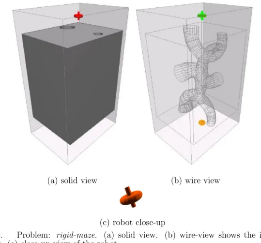
• The rigid-maze problem (Figure 3), has a 6-DOF rigid-body robot that should pass through a series of tunnels with some dead-ends from the top to the bottom. This problem is interesting because its C-Space resembles the workspace, it has two clear free areas, the tunnels form a long and narrow passage with dead ends, and the obstacle occupies the majority of the planning space. Translational-DOF ranges are: x [-8,7], y [-16.5,16.5], and z [-9,11]. Rotational DOFs are not bounded.

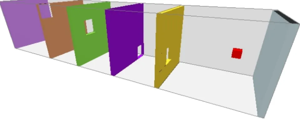
• The rigid-windows problem (Figure 4) has a 3-DOF translational rigid-body cube robot that should pass through any of the four windows in the wall that splits the environment into two halves. This problem is interesting because it has four different pathways from one side to the other and finding one is not enough to achieve the best model. From left to right, the first window is 1.5 times as long as the robot, the second window is 1.75 times as long as the robot, the third window is 2.5 times as long as the robot, and the fourth window is 3.5 times as long as the robot. The width of the wall is the same as the length of the robot. Translational-DOF ranges are: x [-10,6], y [-0.5,0.5], and z [-2.0, 2.0]. Rotational DOFs are not bounded.

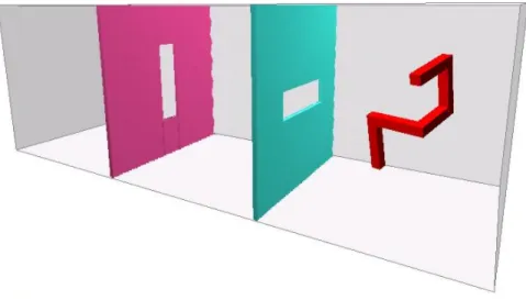
• The rigid-hook problem (Figure 5) has a 6-DOF rigid-body hook robot that should pass through the narrow openings in the two walls that divide the

(43)

envi-(a) solid view (b) wire view

(c) robot close-up

Fig. 3. Problem: rigid-maze. (a) solid view. (b) wire-view shows the internal tunnels. (c) close-up view of the robot.

Fig. 4. Problem: rigid-windows. The robot has 3 translational degrees of freedom. Four pathways of different sizes allow the robot to cross from the front to the back. The start and goal configurations are at each side of the leftmost wall.

(44)

Fig. 5. Problem: rigid-hook. In order to get through the passages, the 6-DOF robot needs to perform translations and rotations.

ronment into three chambers from one side to the other side of the environment. This is an interesting and difficult problem that requires simultaneous transla-tional and rotatransla-tional motions. Translatransla-tional-DOF ranges are: x [-100,100], y [-100,100], and z [-400,200]. Rotational DOFs are not bounded.

• The rigid-walls problem (Figure 6) has a 6-DOF rigid-body box robot that should pass through the small openings (slightly larger than the robot) in the walls that divide the environment into five chambers from one side to the other side. This problem has a C-Space that is similar to its workspace, with four nar-row passages and open spaces in between. Incremental planners increase their coverage in stages as they find their way through the passages. Translational-DOF ranges are: x [0,4], y [0,4], and z [-5,14]. Rotational DOFs are not bounded.

• The serial-hook-5 problem (Figure 7) has five links that form a ten-DOF artic-ulated robot that should pass through the opening in the wall that divides the

(45)

Fig. 6. Problem: rigid-walls. Incremental planners find their in increments as they find their way through narrow passages.

environment into two chambers from one side to the other side of the environ-ment. This is an articulated version of the rigid-hook problem that has a higher number of DOFs than the other problems. Translational-DOF ranges are: x [-100,100], y [-[-100,100], and z [-400,200]. Rotational DOFs are not bounded. • The serial-spring-98 problem (Figure 8) has ninety eight links that form a

103-DOF articulated robot whose start and goal configurations resemble springs of different widths. The robot should pass above a wall that divides the environ-ment into two areas folding and unfolding. The high number ofDOFs makes this problem much harder than any of the other problems discussed. Translational-DOF ranges are: x [-500,500], y [-500,500], and z [-500,500]. Rotational DOFs are not bounded.

C. Experimental Setup

All the experiments were performed in individual processors of the IBM HPC cluster 1600 of Texas A&M University. This cluster runs the 64-bit version of AIX (version 5.3), and it has 40 p5-575 nodes, each with 16 Power5+ processors at 1.9 GHz and

(46)

Fig. 7. Problem: serial-hook-5. The 10-DOF robot can fold and unfold to get through the opening that divides the environment. This is a variation of the rigid-hook problem.

Fig. 8. Problem: serial-spring-98. The 103-DOF robot folds and unfolds to get above the wall that divides the environment.

(47)

32 GBytes of DDR2 DRAM in a shared-memory configuration (SMP). This resource was used for over 600 hours including trial runs and the final experiments shown in this work.

All the techniques were implemented in C++ within the Parasol Lab Motion Planning Library. Validity was evaluated using the RAPID collision detection package [20].

Executions are split into subsets, or bins, of n consecutive iterations to gather statistics and evaluate performance. Times were tracked individually for model gener-ation (node genergener-ation and connection in roadmap-based planners, and expansion in incrementally-exploring planners), metrics computation (node-level, global-level, and region-level), witness-query evaluation, and input/output (to store C-Space models). As mentioned previously, we evaluated the following roadmap-based planners: Basic-PRM, OBPRM, Gauss-PRM, MAPRM, and Bridge-Test. Also, we evaluated the following incrementally-exploring planners: RRT-Expand, EST, RRT-Connect, andRPP. All these planners are described in detail in chapter II. For each planner, we used the parameters that yielded the best performance for each method and problem in preliminary experiments. We applied each planner to an instance of the problem eight times using different seeds for the random number generator, and then we aggregated statistics of the eight runs.

In Section V.A, we evaluate the error with different approximation levels that can be specified in some of the node-level metrics. We executed all the planners in all the problems up to sixteen different times. We noted that even with four different runs we obtained standard deviations smaller than 5%.

In Section VI.A, we illustrate the global-level metrics with the application of Basic-PRM on the simplerigid-windows problem which can be solved through mul-tiple pathways. The planner was executed ten times, and we showed one of the

(48)

executions that illustrates better the identification of multiple pathways. Here, the node-level metrics were computed every bin with an expansion threshold of 0.5 and neighbor-probability test for all connections, the global-level metrics were computed every 10 bins, witness queries were performed every bin. Since the structural changes happen at the initial iterations, we only show metrics for the first 200 nodes.

In chapters V, VI, and VII we show the application of the different metrics to eval-uate the planners and problems described above. In the roadmap-based Gauss-PRM andBridge-Test planners, we used the same value for thed parameter for each prob-lem: d= 10 in therigid-hook problem and in therigid-maze problem; d= 2.16 in the serial-hook-5 problem, andd= 0.2 in therigid-walls problem. In the incrementally-exploringRRT-Expand and RRT-Connect planners, we used the same value for the q parameter for each problem: q = 0.06 in the rigid-walls problem, and q = 0.04 in therigid-hook and in theserial-hook-5 problems. In the incrementally-exploringEST planner we used the following parameters: neighborhood radiusq= 0.04 and number of neighbors to evaluate density k = 5 in the rigid-walls problem; and q = 0.08 and k = 5 in the rigid-hook and serial-hook-5 problems. In the incrementally-exploring RPP planner we used the following parameters: step size q =.05, maximum escape trials t = 20 in the rigid-walls problem; and q = 0.02, and t = 10 in the rigid-hook and serial-hook-5 problems. Each planner was applied 16 times to each problem to gather the metrics. The metrics were computed every 20 bins.

(49)

CHAPTER V

NODE-LEVEL METRICS

Metrics at the node level allow the estimation of changes in coverage and connectivity of the model with the addition of each new node. We can estimate the type and quantity of improvements in the model due to new nodes based on structural changes of the model and on an estimation of the local visibility of the new node. Node-level metrics provide local information around the nodes in the model, but they do not provide information about global coverage, distribution of samples or topology.

A. Type and Amount of Improvement Produced by a New Node

Given a model M, a planner adds a valid sampled configuration v and a selected subset of its valid connections producing the model M0. This operation changes the connectivity and coverage of the original model M in exactly one of the following ways:

1. cc-create —v lies outside the coverage region of all the components in M as seen in Figure 9(c). A new component CC with v as its only node is created. The coverage of M increases by the coverage of v and the connectivity and topology improve due to the new component.

2. cc-merge — v lies inside the overlapping coverage region of more than one component of M as seen in Figure 9(d). As a consequence, the components and their coverage regions merge, reducing the number of components. The coverage of M increases only by the coverage of v and its connectivity and topology improve due to the new pathways found.

(50)

(a) no samples (b) visibility (c) cc-create

(d) cc-merge (e) cc-expand (f) cc-oversample

Fig. 9. Classification of new nodes when modeling the C-Space of a point robot moving in the plane shown in (a). (b) The first sample in the model with its visibility region. (c) A new sample lying outside the visibility region of any other sample creates another component with its own visibility region. (d) A new sample lying in the overlap of the visibility region of two components allows to merge them. (e) A new sample lying inside the visibility region of one component expanding its visibility: cc-expand. (f) A new sample lying inside the visibility region of one component without changing its visibility: cc-oversample.

3. cc-expand —v lies inside the coverage of exactly one component of M and it increases the coverage of the component as seen in Figure 9(e). The coverage of M increases but the connectivity ofM remains constant. The amount of model improvement in this case is the increase in coverage.

4. cc-oversample —v falls inside the coverage of exactly one componentCC in M as seen in Figure 9(f). The coverage and connectivity ofM remain constant. Three of these cases improve the representation of the coverage and/or the con-nectivity of the model: cc-create, cc-merge, and cc-expand. The fourth case,

(51)

cc-oversample, does not represent an improvement of the model as will be shown in our experimental studies. cc-expand andcc-oversample nodes occur very frequently while cc-create and cc-merge nodes are much less frequent. In particular, roadmap-based planners may producecc-createnodes in hard to reach areas andcc-mergenodes when paths between disconnected components are found. Also, incremental planners only produce cc-create nodes when starting a tree and cc-merge nodes when connecting trees or finding a connection to the goal.

In order to accurately classify the nodes, we need to estimate their visibility region. This is unfeasible to compute because it would be as hard as computing the C-Space around the node. However, as we will see, reasonable approximations can be computed efficiently using only local information.

In this work we discuss only one of the many ways in which node classification can be implemented. A node that increases the number of roadmap components is a cc-create node as shown in Figure 10(b). A node that causes a reduction in the number of components in the roadmap is acc-mergenode as shown in Figure 10(c). In order to distinguish cc-expand and cc-oversample nodes, we compute the expansion ratio E(v) for the node v as follows: a node v that connects to a node v0 in the roadmap, but cannot be connected to a percentage Ev,v0 of v0’s neighbors produces

an expansion in the proportion of Ev,v0 as shown in Figure 10(d). We call E_v,v0 the

amount of expansion of v with respect to v0. The expansion ratioE(v) for the node v is the maximum of the expansions produced for all the nodes v0 connected fromv. A thresholdEt is used to distinguish between cc-expand and cc-oversample nodes so that a node iscc-expand if E(v)>=Et, otherwise it is cc-oversample. Most nodes of our preliminary experiments showed anE(v) either close to 0.0 or close to 1.0, so we decided to use a Et = 0.5 in the rest of this work. This way the node v in Figs. 10 (d) and (e) arecc-expand while the nodev in (f) is cc-oversampl