A Novel Ensemble Method for Electric Vehicle
Power Consumption Forecasting:
Application to the Spanish System
CATALINA GÓMEZ-QUILES 1, GUALBERTO ASENCIO-CORTÉS2, ADOLFO GASTALVER-RUBIO 3,
FRANCISCO MARTÍNEZ-ÁLVAREZ 2, ALICIA TRONCOSO 2, JOAN MANRESA4,
JOSÉ C. RIQUELME 5, AND JESÚS M. RIQUELME-SANTOS1
1Department of Electrical Engineering, University of Seville, 41092 Seville, Spain 2Data Science and Big Data Laboratory, Pablo de Olavide University, ES-41013 Seville, Spain 3Ingelectus S.L., 41092 Seville, Spain
4Red Eléctrica de España, 28109 Madrid, Spain
5Department of Computer Science, University of Seville, 41012 Seville, Spain
Corresponding author: Catalina Gómez-Quiles ([email protected])
This work was supported by the Spanish Ministry of Economy and Competitiveness under Project ENE2016-77650-R, Project PCIN-2015-04, and Project TIN2017-88209-C2-R.
ABSTRACT The use of electric vehicle across the world has become one of the most challenging issues for environmental policies. The galloping climate change and the expected running out of fossil fuels turns the use of such non-polluting cars into a priority for most developed countries. However, such a use has led to major concerns to power companies, since they must adapt their generation to a new scenario, in which electric vehicles will dramatically modify the curve of generation. In this paper, a novel approach based on ensemble learning is proposed. In particular, ARIMA, GARCH and PSF algorithms’ performances are used to forecast the electric vehicle power consumption in Spain. It is worth noting that the studied time series of consumption is non-stationary and adds difficulties to the forecasting process. Thus, an ensemble is proposed by dynamically weighting all algorithms over time. The proposal presented has been implemented for a real case, in particular, at the Spanish Control Centre for the Electric Vehicle. The performance of the approach is assessed by means of WAPE, showing robust and promising results for this research field.
INDEX TERMS Time series forecasting, electric vehicle, power consumption, ensemble learning.
I. INTRODUCTION
Nowadays, transport is responsible for around a quarter of the European Union’s (EU) greenhouse gas emissions, being conventional cars responsible for around 12% of EU total emissions of carbon dioxide (CO2) [1]. Transport is the only major sector in the EU where greenhouse gas emissions are still rising [2], becoming therefore a key point for decarboniz-ing the European economy [3]. One of the 2021 objectives of the EU consists in a 40% decrease in emissions from new cars compared to 2005.
At world level, in 2015, 1.26 millions of electric vehi-cles (EV) were on the roads. Electric cars include battery electric (BEV), plug-in electric (PEV), plug-in hybrid elec-tric (PHEV), and fuel-cell elecelec-tric vehicles [4], [5]. The EV The associate editor coordinating the review of this article and approving it for publication was Emanuele Crisostomi.
growth up to date has followed an almost exponential trend, having in 2014 almost half of the EV available today, and being counted in 2005 by hundreds. Other type of vehi-cles, like the freight delivery vehivehi-cles, electric buses, or the 2-wheelers are also taking importance in some regions, as for example in China, where the latter represent 200 millions of units in stock [6]. Today, 80% of the electric cars on road worldwide are located in the United States, China, Japan, the Netherlands and Norway. In Spain, more than 19,000 EV were in use at the end of 2015, including delivery vehicles and electric buses [7]. The fast growth of this type of technology is due to the success of incentive policies, which have led to the development of this type of transport, achieving lower costs, greater accessibility to charging points, greater autonomy in vehicles, and higher loading speeds, making the EV an increasingly attractive product for the consumer.
The EV will gain a foothold in the electricity systems and will conform a new type of load, which behaves in a very different way than conventional loads. During the peak hours, these vehicles usually are on the roads. Moreover, during the valley hours (when demand levels are lower), they are usually recharging.
The uncontrolled charge of the EV fleet may become into some threat of power-outages for some systems with a weak electricity infrastructure if they coincide with a peak of demand and with hours in which the renewable penetration is low (hours in which the cost per kWh is higher, and in which sufficient back-up generating power has to be avail-able). In the European system, a small scale EV introduction (up to 5% of the fleet) will not pose a significant threat to mature distribution grids [8]. However, controlled charging will allow a much greater number of cars in the systems without local overloading.
In order to manage the demand power supply in an efficient and safe manner, the generators need to be programmed in advance in order to fulfil with the demand levels, in an environment in which electricity markets provide provisional programs that needs to be updated in real time due to the uncertainty associated to both generation and demand. For this reason, the prediction of renewable energy penetration, as well as the prediction of EV consumption [9], is crucial. The former has been widely studied during the last years. New tools, such as the renewable generation aggregators, have been developed in order to reduce the risks associated with the uncertainty the renewable generation presents. As the EV consumption takes more presence, the prediction of the aggregated EV demand gets more important for the Trans-mission System Operator (TSO).
In this paper, the focus will be put on the forecast of the electric vehicles power consumption. In particular, three well-established algorithms –ARIMA, GARCH and PSF– are used in a combined way in order to predict the EV power consumption, with specific application to the Spanish system. The proposal presented has been implemented at the Span-ish Control Centre for the Electric Vehicle (CECOVEL, https://goo.gl/h79jdE), recently created by the Spanish TSO, Red Eléctrica de España (REE). This center integrates the impact of the massive deployment of electric vehicles in the system, complementing this way the activities of the Elec-tricity Control Center (CECOEL), responsible for the coor-dinated operation and real-time monitoring of the generation and transmission facilities of the national electricity system.
In order to integrate the maximum amount of gener-ation from renewable energy sources into the electricity system, while ensuring quality levels and security of sup-ply, in mid-2006 REE designed, put in place and started the operation of the Control Centre of Renewable Ener-gies (CECRE, https://goo.gl/QxxDqk), a pioneering center of world reference regarding the monitoring and control of renewable energies. It is worth noting that this project has received recognition in the Smart Vehicle category of the 2017 enerTIC Awards (winner at Smart Vehicle
category, https://goo.gl/pGmx5R), a prestigious venue focused on projects with high commitment with innovation and energy efficiency and sustainability. Furthermore, this approach is currently working on a real-time basis for EV managing in some centers in Spain.
Reported results show the performance of the ensemble developed and its ability to adapt to the non-stationary nature of the time series analyzed.
In short, the contributions of this paper can be summarized as follows:
1) Development of a new algorithm to forecast EV power consumption. The algorithm applies ensemble learn-ing to combine three existlearn-ing algorithms, that have already been shown to be useful in the power consump-tion context, through a weighted least squares (WLS) adjustment.
2) Since the number of charging points is continuously growing, non-stationary time series must be analyzed. Ensemble weights are periodically updated in order to deal with this tough problem.
3) Application for the first time to data from Spain, a country which is currently investing much money in the deployment of EV, with a rapid growth penetration. 4) Winner of several awards and actual implementation
and real-time usage at Spanish CECOVEL.
The rest of the paper is structured as follows. SectionII
reviews recent and relevant works related to electric vehicle consumption forecasting. A description of Spanish EV data can be found in SectionIII, along with an explanation on how these data are collected. The proposed methodology is described in Section IV. Section V reports the results achieved from the application of the proposed methodology to Spanish data. Finally, all conclusions drawn from this work are summarized in SectionVI.
II. RELATED WORKS
This section describes related works that justify the need of developing a new methodology, such as the one here proposed.
Regarding the trends and the consequences the future EV penetration levels will cause in the network, several works have been proposed. In [10], the impact of electric vehicles charging on electricity consumption is analyzed, modeling the generation planning and the concentrated power demand (in time and space) at specific points of the network, and highlighting the specific situation in Hungary.
In [11], the development status and trends of PEV in China is introduced first, followed by the analysis of the supply modes of different kinds of PEV in China, using Monte Carlo simulations to determine the initial charging point based on probability distributions of starting charging time, and con-cluding that the charging of EV will pose significant impacts on the power grid in 2030 in China.
In [12], an approach to model frequency regulation (FR) via Vehicle-to-Grid (V2G) on a large scale is presented, with an emphasis on forecasting the availabilities of the vehicles
at hour-long intervals, including route locations, and states of charge.
As for specific forecasting techniques applied to EV fore-casting, a brief introduction of characteristics of the charging station is given in [13], based on the daily load data of Beijing Olympic Games EV Charging Station in 2010, and establishes three types of daily load forecasting model for EV charging station load [14]: backpropagation neural network, radial-basis function neural network, and Grey Model(l, 1).
In [15], a short-term load forecast model using Sup-port Vector Machines and artificial intelligence technique is proposed, evaluating the accuracy of the results through a comparison with a Monte Carlo forecasting technique. By contrast, in [16], the same authors examine the use of various data mining methods and their performance in EV load forecasting.
In [17], the Modified Pattern-based Sequence Forecast-ing (MPSF) is compared with the k-Nearest Neighbor (kNN), the Support Vector Regression (SVR) and the Random For-est (RF) to predict the energy consumption at individual EV charging outlets using real world data from the University of California, Los Angeles campus. In [18], the same authors include also the ARIMA algorithm and Pattern Sequence Forecasting (PSF) in their analysis.
Duan et al. [19] first forecasted electricity market param-eters, as well as the diurnal recharging load curve, by using ARIMA and, later, with a fuzzy algorithm showing remark-able improvements. They used synthetic data for 10000 EV located at Texas. Authors claimed that their approach is capa-ble of dealing with market uncertainties.
The risks of day-ahead scheduling and real-time dispatch EV charging are addressed in [20]. The authors were con-cerned about the growing exponential complexity associated with the number of EV. For this reason, they proposed a dis-tributed approach to optimize the charging strategy. Another key point is the sampling methodology they proposed in order to reduce the costs.
Big data technologies have also been used in this context. In 2016, Arias and Bae [21] introduced an algorithm to forecast EV charging demand. Data from historical traffic and weather were used as input and several machine learning algorithms (clustering, relational analysis or decision trees) were used to improve such estimation. Data from South Korea were used to assess the performance of the approach, showing satisfactory results.
The use of SVR for charging load forecasting of EV sta-tions has also been analyzed in [22]. The authors proposed a simple but effective model based on historical data, in which they considered multiple variables such as number of EV, weather, historical charging loads or properties of the week.
One year later, SVR was also applied but, this time, a meta-heuristic based on genetic algorithms and particle swarm optimization was used to set the algorithm [23]. Several new variables were considered, such as air quality. Real data from China were analyzed and results showed that the use of the metaheuristics deeply improved the results.
A real-time forecasting of EV charging station scheduling approach can be found in [24]. In particular, the authors developed an interactive user platform to allocate the charg-ing slots based on estimated battery parameters, which uses data communication with charging stations to receive the slot availability information. The platform, implemented in a low-cost microcontroller, provides real-time information to prevent halting for low battery reasons.
Also in 2017, Arias and Bae [25] proposed a novel time-spatial model to predict EV charging-power demand, in realistic urban traffic networks, at fast-charging stations. In particular, real-time closed-circuit television data from Seoul (South Korea) were used to assess the performance of the approach.
A new approach to forecast electricity demand of EV was introduced in [26]. The authors analyzed charging patterns from customers, thus finding different profiles depending on customers type (public and private). Two main conclusions were drawn: first, faster EV supply equipment during peak load time is preferred and, second, tradeoffs between charg-ing time and price are considered.
A day-ahead forecasting model for probabilistic EV charg-ing loads at business premises can be found in [27]. Hence, several approaches were combined to estimate different statistical parameters, based on historical data. From the reported results, the authors claimed that this method can reduce the number of decision variables, and require less computational time and memory.
Another interesting energy optimization proposal for EV in smart cities can be found in [28]. The main idea underlying the approach is that EVs and buildings can share some par-ticular information regarding both vehicle and roads status. By processing such information EVs can be classified and buildings can make recommendations according to their posi-tions. Another smart database for power management EVs by the same authors can be found in [29].
Ejaz and Anpalagan [30] proposed a new methodology for EV charge scheduling in smart distribution systems, based on the internet of things paradigm. Two main features were taken into consideration to achieve the goal: charging speed and cost within the stations. The goal was to maximize benefits while minimizing costs.
None of the mentioned works is aimed to forecasting hourly EV demand using as input data real EV consumption gathered by the TSO, aggregated at country level. This spe-cific time series presents particular characteristics, described next, that justify the need of a new forecasting methodology that fits its behaviour.
III. ELECTRIC VEHICLE POWER CONSUMPTION
Nowadays, most of electric vehicles are charged in EV charg-ing stations (also known as chargcharg-ing points). Each station is capable of detecting whether an EV has been connected, and measuring the accumulated energy consumption since its connection. In this paper, the period since the EV is connected
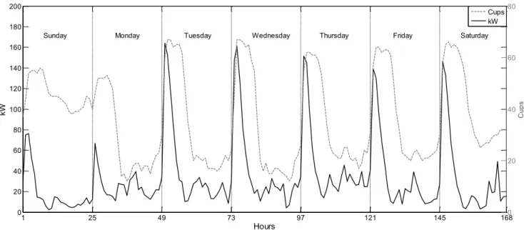
FIGURE 1. Typical week of electric vehicle power consumption (left y-axis) and number of cups (right y-axis).
until it is disconnected, regardless of its state of charge, is calledconnection attempt.
Charging stations are spread all over the geography in order to give service to the EV, whose limited autonomy is currently one of the main research objectives in the EV-development field. From the point of view of the power system, the dis-tributed charging points can influence the operation of the distribution networks.
In order to generate a proper time series, the connection attempt data set is filtered and accumulated by hour and geographical zone. Thus, in a geographical zone, for each hour of the year, there is a single calculated value, which is the measured EV power consumption.
Real data from different geographical zones have been aggregated in order to get a single time series, correspond-ing to the total energy consumption of all the Spanish EV. In particular, the real consumption data of the dif-ferent charging points available in Spain have been pro-vided by Spanish Public Grid (Red Eléctrica de España,in Spanish).
The resulting time series presents a weekly pattern, as shown in Fig. 1 (solid line), where the Spanish EV power consumption from Sunday 6th to Saturday 12th of March 2016 is represented (left y-axis). As can be seen, Sundays and Mondays present a different pattern than the rest of the days, in which a peak value appears during the first 6 hours of each day, this is, during the night hours. On the same graph, the right y-axis represents the number of cups that keep connected (dotted line), regardless the level of charge. By comparing both curves it can be observed that the consumption peaks decrease before the number of cups do, those last remaining high until 8 am during the working days, and during the Sundays. This means that a large number of EV remain connected after the charge is completed.
This behaviour can be explained since the EV are in use during the working hours of the week days (Mondays to Fridays), and they are usually recharged during the following night.
One of the particularities of this type of load is that it takes high values during the night hours, since the EV are put to recharge when they are not being used. The behaviour of this new massive electricity consumer is the opposite to that presented by the majority of electricity consumers.
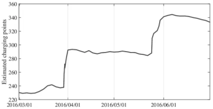
In Spain, the current time series of demands for electric vehicles is evolving given that the number of existing electric vehicles as well as the number of recharging points is in full growth. The tele-acquisition of data by the system operator is in full evolution and, for this reason, the time series presented by the integrated demand of EV at the Spanish level is non-stationary, which greatly complicates its characterization and, therefore, its prediction over time.
Figure2shows the number of charging points from which data has been received during the months of study. As can be observed, the trend of number of charging points in use is growing, but the series is not monotically increasing. This fast evolution in the amount of data available produces a non-stationary time series, continuously changing, which hinders the forecasts based on historic data.
IV. METHODOLOGY
In this paper, the power consumption of the Spanish electric vehicles is predicted using an ensemble composed of different approaches: PSF, ARIMA and GARCH algorithms.
First, the ARIMA, GARCH and PSF algorithms will be used to forecast the EV consumptions of months March to May 2016 in Spain. At each hour of each day during this period, predictions with a forecast horizon of 48 h will be made (from the hour after the time the prediction is
FIGURE 2. Estimated charging points.
executed onwards). For each simulation, a 1 year back histor-ical data will be available. The effect of updating the models of the algorithms based on time series (ARIMA and GARCH) will be evaluated.
Then, the results from the previous simulations will be compared to the result of combining the three algorithms in order to get a weighted prediction. To do so, an ensemble will be developed, which will weight the different algorithms comparing the predictions made during the previous week with respect to the real consumptions during that hours, through a weighted least squared process. A 1-week window is used for the comparison given the speed at which the time series is changing. The need of updating at each simulation the calculated coefficients will be evaluated, and the results will be compared with the option of averaging the predictions of the three algorithms.
The real consumption data of the different charging points available in Spain have been provided by REE, for the devel-opment of the CECOVEL project.
All simulations have been developed in Matlab environ-ment, version 2013, with the following Toolboxes included: Econometrics Toolbox (ver. 2.4) Financial Toolbox (ver. 5.2) Image Processing Toolbox (ver. 8.3) MATLAB Compiler (ver. 5.0) Neural Network Toolbox (ver. 8.1) Optimization Toolbox (ver. 6.4) and Statistics Toolbox (ver. 8.3).
In the following subsections, the methodology followed to implement each algorithm (SectionIV-Ato SectionIV-C) and the ensemble (SectionIV-D) is presented.
A. ARIMA
This model is based on three main pillars: the autoregressive model (AR), the moving average model (MA), and the differ-entiation of the time series.
An AR model of orderp predicts the value of a variable through a weighted sum of the p values previous to this variable:
AR(p)=Xt =81Xt−1+82Xt−2+. . .+8pXt−p+at (1)
This way, an AR model is defined by its orderp, and the values of the coefficients8i withi = 1, . . . ,p. Equation 1
shows that the value of the variable of interest at time instant t is obtained as the sum of the value of this variable in
the previous instant, multiplied by the coefficient81, plus the value of this variable in the two-times previous instant multiplied by82. . . , and so onptimes.
A MA model of order q predicts a variable through a weighted sum of theq previous values of the errorsai that
occurred when forecasting:
Xt =at−v1at−1−v2at−2−. . .−vqat−q (2)
The MA model is defined by its orderq, and the values of the coefficientsvi, withi=1, . . . ,q. Equation2shows that
the value of the variable at instanttis obtained as the sum of the error at the previous instant multiplied by coefficientv1, plus the value of the error two instants before multiplied by coefficientv2. . . , and so onqtimes.
An ARMA model has both the AR- and the MA- com-ponents. When using differentiated time series, the model is called ARIMA (Autoregressive Integrated Moving Average). As shown in Equation3, it combines an AR model (left-hand side term) with a MA model (right-hand side term), applying operator (1−Bd), which consists in differentiatingdunits the time series.
(1−81B−82B2−. . .−8pBp)(1−Bd)Xt
=(1−v1B−v2B2−. . .−vqBq)at (3)
Once a forecast is provided, the differentiation has to be undone in order to get the forecasted time series. A 1-week differentiation will be applied, given the weekly seasonality shown by the time series of electric vehicle power consumption.
B. GARCH
The GARCH model (Generalized Autoregressive Condi-tional Heteroskedasticity) assumes that the error of the vari-ance fits an ARMA process. A GARCH (p,q) is a model for conditioned variables, wherepis the order associated to the past variances,σ2, and q is the order of the ARCH terms associated to the squared innovations,2. A (p,q) GARCH model is given by: σ2 t =α0+α1t2−1+. . .+αq2t−q+β1σt2−1+. . .+βpα2t−p =α0+ q X i=1 αit2−i+ p X i=1 βiσt2−i (4)
Since this model is suitable for zero-mean processes, it will be applied to a 1-week differentiated time series. This way, a differentiated forecast will be obtained, which must be added to the recorded real data of the previous week in order to get the final forecasted time series.
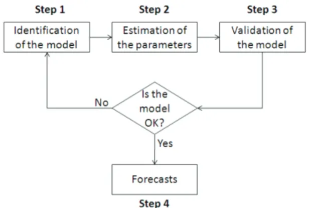
A flowchart of the ARIMA and GARCH methodology is shown in Figure3.
C. PSF
An initial version of the Pattern Sequence-based Forecasting algorithm (PSF) was proposed in [31], but it was not until 2011 when it was finally published [32]. An improvement can
FIGURE 3. ARIMA and GARCH flowchart.
be found in [33] and its implementation in R is available in [34], [35].
The main feature of PSF lies in its ability of predicting time series with arbitrary prediction horizons with robust performance regardless of how long the horizon is. Addi-tionally, it must be considered that this algorithm performs better when time series exhibits certain temporal patterns, since its development is directed towards the discovery of these patterns.
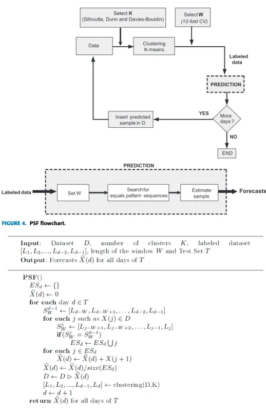
PSF consists of several clearly differentiated steps: 1) Data transformation. Data must be transformed into a
d ×h matrix, where d denotes the number of days considered andhthe number of hours. Note that PSF can be applied to data of any structure by, for simplicity, d×hvalues are assumed, as in the original work. 2) Clustering. The K-means algorithm is later applied to
such transformed matrix. That way, every day is identi-fied by a label (the one generated during the clustering process). Note that the election of the numbers of clus-ters is critical and a majority system vote is proposed within the original manuscript to determine the optimal value. Silhouette, Dunn and Davies-Bouldin are the indexes used.
3) Selecting the length of the pattern sequence or slid-ing window. The second key issue in PSF consists in determining how long the pattern sequence must be. In this particular case, the pattern sequence stands for the number of consecutive labels (those generated by clustering and identifying consecutive days in the historical data) that PSF must retrieve to search for it in the historical data. The optimal value for this parameter is calculated by means of 12-fold cross validation.
4) Prediction. Once the number of clusters and the length of the window are determined, the prediction can be made. To reach this goal, PSF searches for the pattern sequence within the historical data and, every time a hit is found, values for the nexthhours are picked. The prediction itself is the average value for all hits. Finally, the flowchart and pseudocode for PSF can be found in Figures4and5, respectively.
D. DEVELOPING OF THE ENSEMBLE MODEL
The predictions provided by the three methods have been combined in order to obtain a weighted forecast. With this objective, an ensemble module has been developed, which calculates the weighting coefficients to be applied to each method and each hour of the forecast horizon. Assuming a 48-hour forecast horizon, this means 48×3 coefficients to be calculated. The process implemented consists in a weighted least squares adjustment by comparing the predictions of the three algorithms obtained during the previous week (7×24 48-hour predictions for each method) with respect to the real power consumptions observed during the 48 h horizon corresponding for each simulation. This way, for each hourh of the forecast horizon, the three corresponding coefficients are obtained by solving the following equation:
Ach =b (5)
beingcha 3×1 column vector containing the three
coeffi-cients for hourhassociated with the three prediction methods;
Aa matrix with three columns, one per method, and whose rows are the 24×7 predictions associated to hourhprovided by the corresponding algorithm at each simulation, according to the past predictions history;bis a column vector containing the 24×7 samples of real power consumption at hourhof the horizon of prediction at each simulation.
This way, the weighted prediction consists in a linear com-bination of the three algorithms.
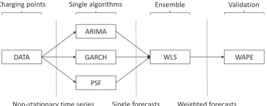
Finally, Figure 6 illustrates the proposed methodology. It can be observed that, firstly, data from charging points are collected. Since the number of these points is continuously growing, the time series generated are non-stationary. Such series serve as input for ARIMA, GARCH and PSF, which generate their own forecasts. Later, results for these three algorithms are combined by means of an ensemble, making use of WLS. The final output, the weighted forecasts for every single algorithm, is validated by means of a well-known metric: Weighted Absolute Percentage Error (WAPE). E. BENCHMARK ALGORITHMS
In order to show the effectiveness of the ensemble algorithm proposed, a set of five algorithms were added as benchmark to the experimentation carried out. These algorithms were trained and tested on the same data partitions and experi-mental setting used to test the proposed ensemble, for a fair comparison.
The benchmark algorithms were selected from the classic machine learning literature and are purposed to the super-vised learning task of regression. These algorithms were: Random Forests, including an ensemble of 10 trees for regression (RF10), Nearest Neighbors algorithm with k=1 (KNN1), Locally Weighted Learning algorithm (LWL), Sim-ple Regression Tree (SRT) and Multilayer Perceptron algo-rithm for artificial neural networks (MLP). Below is shown a brief description of them.
The algorithm RF10 is the classic random forests ensem-ble built on regression trees using the bagging technique
FIGURE 4. PSF flowchart.
FIGURE 5. PSF pseudocode.
proposed in [36]. The algorithm was configured to include 10 unpruned trees.
The KNN1 algorithm is the nearest neighbours approach applied to regression tasks as it was proposed in [37]. The algorithm was set for considering one nearest neighbour (k=1) and no distance weighting.
The LWL algorithm is a case-based reasoning approach that firstly assign weights to the input instances and then
does linear regression minimizing the mean-squared error weighted by the previous instance weights assignments. This algorithm were proposed in [38].
SRT is a algorithm that constructs a regression tree fol-lowing the procedure of the algorithm M5’ proposed in [39], using the default configuration described in such work.
The algorithm MLP constructs an artificial neural net-work using the multilayer perceptron classic algorithm [40].
FIGURE 6. Flowchart of the proposed methodology.
The algorithm produces a model that is a feed-forward back-propagation neural network using an stochastic gradi-ent descgradi-ent optimizer and an architecture that includes one hidden layer with (n+c)/2 neurons (wherenis the number of input features andcthe number of classes, which is 1 for regression).
V. RESULTS
The algorithms ARIMA, GARCH and PSF, described in the previous section, have been used to perform 48-hour day ahead predictions (48-hour forecast horizon) at each hour of the months March to May 2016. The election of this prediction horizon was made according to particular needs that REE requested.
For the ARIMA and the GARCH algorithms, the param-eters of the corresponding models have been calculated by using a one-year length electric vehicle power consumption observations. Given the patterns observed in the weekly time series, two models have been defined for each algorithm: one for Sundays and Mondays (SM models); and one for Tuesdays to Saturdays (TS models), which is also a common strategy in this scenario [41]. This implies that the differen-tiated time series is split into two subseries, one containing all Sundays and Mondays to calculate the SM models; and another containing the rest of the days for calculating the TS models. For the SM and the TS models, the (p,q) orders considered for both algorithms are (48, 48) and (120, 120) respectively.
In the PSF algorithm, the number of clusters,K, and the length of the window,W, are continuously recalculated for each simulation, as the historic of data increases in time. This update is automatically performed whenever the PSF simulation is required.
The rest of the section is structured as follows. SectionV-A
introduces the quality parameters used to compare the good-ness of each algorithm. The prediction accuracy individ-ually achieved by each algorithm (ARIMA, GARCH and PSF) is shown and explained in SectionV-B. The proposed ensemble were tested using different weighting schemes and results are shown in Section V-C. The proposed ensemble
with its best weighting scheme is compared with the set of benchmark algorithms in terms of effectiveness in SectionV-D. In V-E, the maximum and minimum errors obtained when applying the best combinations of models and weighting coefficients will be evaluated. The weighting coefficients obtained were analysed inV-F. Finally, the con-vergence of the error achieved by the proposed ensemble is analzsed in SectionV-G.
A. QUALITY PARAMETERS
The goodness of the predictions will be evaluated through the Weighted Absolute Percentage Error (WAPE) [42], which, for a 48-hour prediction performed at hour h, can be cal-culated as follows. Although relative errors could be used for this purpose as well, absolute errors are relevant in this context, since it is needed to know the deviation in MW for a better load generation planning. WAPE is defined as follows:
WAPE(h)= MAE(h) PMEAN(h)
(6) wherePMEAN(h) is the mean value of the real power
con-sumption during the 48-hour prediction horizon:
PMEAN(h)=mean(dsh) (7)
beingdshthe vector with the observations of the historical
data from hourh+1, with length 48; and the Mean Absolute Error (MAE(h)) for the prediction performed at hourh, which can be calculated as follows:
MAE(h)=mean(|dsh−ph|) (8)
beingph the 48-hour prediction vector, from hourh+1
onwards.
B. ENSEMBLE WITH ARIMA, GARCH AND PSF
For a simulation performed at hourh, historical data of elec-trical vehicle power consumptions up to hourhis considered available. The resulting predictions will cover from hourh+1 up to hourh+48.
Predictions at each hour of March, April and May 2016 have been obtained with the three methods. Two different
TABLE 1. Mean and std. of the WAPEs with ARIMA and GARCH models obtained at the end of February.
TABLE 2. Mean and std. of the WAPEs with model parameters of ARIMA and GARCH updated at the beginning of each month.
scenarios will be compared: 1) keeping fixed the models obtained at the end of February for the three-month simula-tions; 2) For each month, updating the ARIMA and GARCH models at the end of the previous month. Note that the PSF model is automatically updated. The WAPEs have been cal-culated for each simulation.
Table1shows the monthly mean values and standard devi-ations (Std.) of the WAPEs for the first scenario.
As can be observed, the ARIMA algorithm presents the largest WAPE values (both means and standard deviations). With the PSF approach the errors decrease with time, while with the ARIMA and the GARCH algorithms, which are based on time series, errors in April show to be lower than errors in presented in May. In all cases, March is the month with largest errors. Given the seasonality of the time series, the models calculated for predicting one month may become outdated for predicting the subsequent months.
Table 2 shows the mean and standard deviations of the WAPEs obtained in the second scenario.
As can be observed, the GARCH model doest not present a significant improvement as a consequence of the model updating, while the ARIMA algorithm improves its errors, specially during April. Despite the updated models, the errors presented in May are still larger than those presented in April.
C. WEIGHTING SCHEMES
The forecasts of the three algorithms have been weighted following three different approaches:
• 1/3 coefficients: Making a simple mean of the
pre-dictions, that is, using weighting coefficients equal to 1/3 for each method and each hour of the forecast horizon.
• Fixed coefficients: Through a weighted average,
cal-culating the 48x3 weighting coefficients at the begin-ning of each month using the ensemble presented in SectionIV-D, and keeping fixed these coefficients for all the simulations performed during that month.
• Updated coefficients: Through a weighted average, updating the 48x3 weighting coefficients at the begin-ning of each simulation.
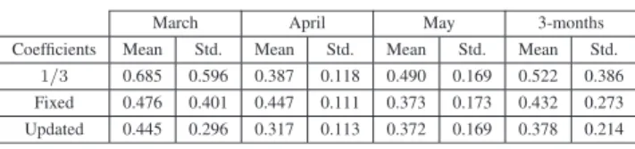
TABLE 3.Mean and std. of the WAPEs with weighted methods, with models updated at the beginning of each month.
Table3present the monthly mean and standard deviations of the WAPEs for the three approaches.
It can be observed that the lower errors are obtained when using updated weighted coefficients which, as explained in SectionIV-D, are based in a weighted least squared adjust-ment of the predictions performed during the previous week with respect to the corresponding real consumptions. Com-paring this result with respect to the best individual monthly solutions it can be found that the PSF model shows bet-ter means for March and May; and the GARCH algorithm shows a better standard deviation for May. At a first look, the weighted solution does not always give the best solution. Let’s analyse the average of the three monthly mean WAPEs and standard deviations for the best approach of the single algorithms (this is, with the models updated for each month) and the best approach of the weighted solu-tion (updated weighting coefficients). Table 4 shows these averages.
As can be seen, in a three-month average, the weighted solution gives in general better results than the individual algorithms. Although at one specific month or hour one of the algorithms may provide a better prediction, it is not possible to know in advance which method will give the best result. The weighted solution is better in long-term averages, as well as in deviations, which implies more robustness.
The increasing trend of the number of charging points (see Figure2) can affect the predictability of the EV con-sumption time series. For such aim, the proposed ensemble was designed, as it was explained before, with the ability to change dynamically the weight assigned to PSF, GARCH and ARIMA according to the most recent values of the series (updated coefficients). As result of such weighting scheme, the WAPE error, averaged for the three tested months, was improved from 1.148±0.7 (ARIMA), 0.394±0.26 (PSF) and 0.398±0.28 (GARCH) to 0.378±0.214 (ensemble with updated coefficients).
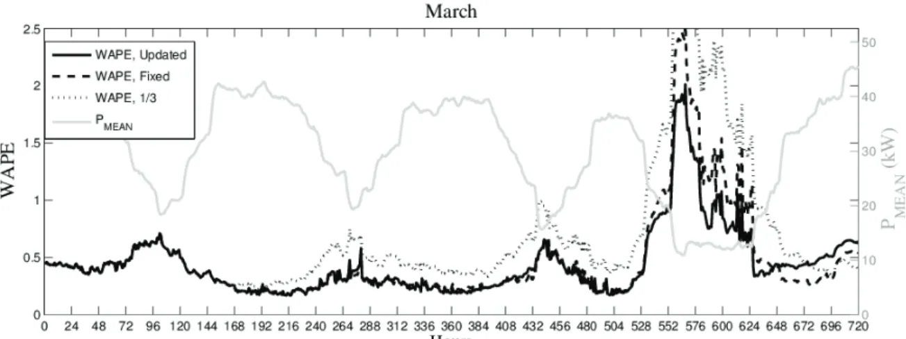
Figures7to9show the evolution of the WAPEs throughout each predicted month.
As can be observed, the WAPEs increase with the hours of lower mean power consumption, as expected from the WAPE definition.
D. COMPARISON WITH BENCHMARK ALGORITHMS The proposed ensemble with its updated weighting scheme was compared with the five benchmark algorithms described in sectionIV-E.
FIGURE 7. WAPEfor March 2016, using different approaches for weighting the different algorithms.
FIGURE 8. WAPEfor April 2016, using different approaches for weighting the different algorithms.
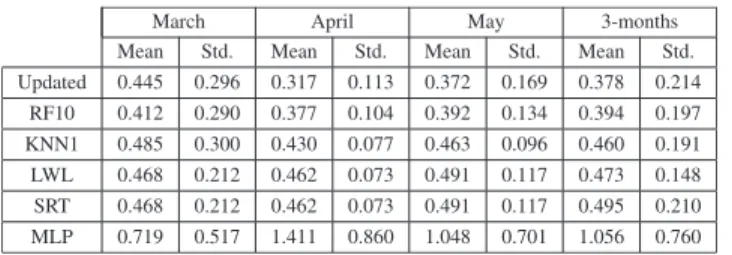
TABLE 4. Comparison of mean and std. of the WAPEs with respect to other algorithms.
The same hours of March, April and May 2016 using the same input data were predicted by benchmark algorithms for a fair effectiveness comparison with the proposed ensemble. In Table4the WAPE values achieved by both the ensemble and each benchmark algorithm are shown. The average and standard deviation of WAPE values are indicated for each month and for all three months averaged (column 3-months). As it can be seen in Table 4, the updated version of the proposed ensemble achieved the best predictions, in terms of the averaged WAPE for the mean of the 3 months.
It is also noticeable that our ensemble proposal was more effective than the random forests algorithm (RF10), which is an ensemble of regression trees, except for the month of March (0.412±0.290 versus 0.445±0.296). A possible rea-son could be that GARCH and PSF (algorithms included in the proposed ensemble) achieved better performance individ-ually (0.398±0.28 and 0.394±0.26, respectively in Table1) than the algorithm SRT (0.495±0.21 in Table4), which is basically the regression tree model aggregated by the random forests algorithm.
RF10 achieved similar results to GARCH and PSF, but it overcame ARIMA. In fact, all the five benchmark algo-rithms overcame ARIMA. For that reason, alternative ensem-bles were constructed replacing ARIMA for RF10, KNN1, LWL, SRT and MLP (five alternative ensembles in total) and keeping GARCH and PSF. Results achieved with these five ensembles did not present significant differences with the proposed ensemble with ARIMA, GARCH and PSF.
E. BEST AND WORST FORECASTS
The best and the worst forecasts obtained during the three-month hourly simulations are analysed. For these simulations, the updated models (at the beginning of each month) as well as the updated weighting coefficients (at the beginning of each simulation) are used, this is, the combination which has shown the best performance in the analyses performed during the previous sections.
Figure 10shows the 48-h prediction with largest errors, which has been performed on March 24th, 2016, at 14:00 h. The 48 hours represented correspond to national holidays: the Holy Thursday from 14:00 onwards; the Holy Friday; and some hours of the Holy Saturday, presenting a WAPE of 2.0131. During these days, the real electric vehicle power consumption is lower than expected.
FIGURE 10. Worst predicted day.
FIGURE 11. Best predicted day.
Figure11shows the prediction with lower errors, which has been performed on Monday, May 9th, 2016, at 12:00 h. The 48 hours represented correspond to conventional week days, presenting a WAPE of 0.146.
F. WEIGHTING COEFFICIENT ANALYSIS
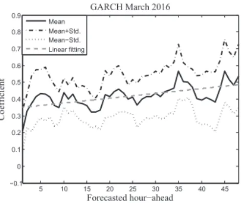
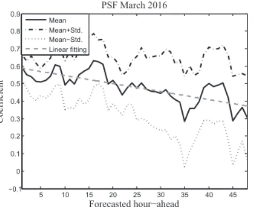
In this section, the monthly mean values and standard devia-tions of the 48 updated weighting coefficients calculated for each method are analysed (Figures12to20), where the black solid lines represent the monthly averages; the black dotted lines represent the± average standard deviations; and the grey dashed lines represent the linear fitting of the monthly averages.
As can be observed, the average hourly coefficients obtained for the simulations of each month corresponding to the ARIMA algorithm are lower than those obtained for the others. This makes sense given the ARIMA algorithm is the one presenting the largest errors. Its average coefficients are close to zero from hour 2 onwards, and present a very flat pattern.
The GARCH and PSF algorithms show coefficients with similar order of magnitude, and with larger standard devi-ations than the ARIMA algorithm. Therefore, these two methods have a similar performance. As can be observed,
FIGURE 12. Mean and standard deviation of the ARIMA coefficients for March 2016.
FIGURE 13. Mean and standard deviation of the ARIMA coefficients for April 2016.
FIGURE 14. Mean and standard deviation of the ARIMA coefficients for May 2016.
when the values of the coefficients of the GARCH method increase, those of the PSF decrease. During the weighting process, the weight falls on one or on the other algorithm, depending on who dominates at that time.
Looking at the linear fittings, it can be seen how the GARCH algorithm shows an increasing trend within the forecast horizon, while the PSF algorithm shows a decreasing trend. This means that, in average, during the first hours the PSF is the predominant method, while the GARCH algorithm takes over while progressing in time.
FIGURE 15. Mean and standard deviation of the GARCH coefficients for March 2016.
FIGURE 16. Mean and standard deviation of the GARCH coefficients for April 2016.
FIGURE 17. Mean and standard deviation of the GARCH coefficients for May 2016.
G. ERROR CONVERGENCE OF THE ENSEMBLE
The proposed ensemble with its updated weighting config-uration was deeply analysed, in order to determine its error distribution across the prediction horizon. Specifically, aver-age and standard deviation of MAE for each predicted hour-ahead are shown in Figures21(March 2016),22(April 2016) and23(May 2016), where x-axis ranges from hour 1 to 48 (48-hour prediction horizon).
As it can be observed in Figures21,22and23, the mean MAE is highly stable across the 48 hours of the prediction
FIGURE 18. Mean and standard deviation of the PSF coefficients for March 2016.
FIGURE 19. Mean and standard deviation of the PSF coefficients for April 2016.
FIGURE 20. Mean and standard deviation of the PSF coefficients for May 2016.
horizon and it converges to 10 kW. This behaviour is very desirable for a predictive model, because the error do not increases significantly when the predicted value is far from the last observed value. Moreover, the deviation of the does not increase either. In fact, such deviation also converges approximately to 10 kW.
In addition, the distribution of error were analysed for each equal-length interval of the predicted variable (electric load of the EV). Specifically, boxplots were used to show the MAE distribution for each interval of the electric load in Figure24. Furthermore, Figure25shows an histogram of WAPE errors for the same intervals. Both figures show the error distribution
FIGURE 21. Mean and standard deviation of the Updated MAEs for March 2016.
FIGURE 22. Mean and standard deviation of the Updated MAEs for April 2016.
FIGURE 23. Mean and standard deviation of the Updated MAEs for May 2016.
for each method: ARIMA, GARCH, PSF and the updated weighting ensemble.
According to the distribution shown in Figure24, it can be concluded that the error of the updated ensemble is distributed in a similar way to GARCH. In turn, GARCH showed the most balanced distribution of error across the range of values of the electric load. Moreover, it is relevant to highlight here that the averaged standard deviation of error of the ensemble (0.214) is lower than those of GARCH (0.28).
ARIMA showed a different distribution of errors with respect to the rest of the algorithms. The ARIMA errors does not converge to any specific value across all the intervals analysed. Namely, the error distribution was significantly different depending on the actual value of the electric load.
FIGURE 24. Boxplots of the MAE error distribution produced by ARIMA, GARCH, PSF and the proposed ensemble with updated weighting for each interval of the predicted variable (Load).
FIGURE 25. Histogram of the WAPE error distribution produced by ARIMA, GARCH, PSF and the proposed ensemble with updated weighting for each interval of the predicted variable (Load).
Figure 25confirms that the same behaviour occurs for the WAPE error.
VI. CONCLUSION
A new methodology has been developed for predicting the EV consumption in an environment in which the historical data is evolving due to the rapid evolution of the penetra-tion of this technology in the system. The study has been carried out with real data of the EV power consumption in Spain.
The algorithm developed has been implemented in the Electric Vehicle Control Center recently created by the Span-ish TSO (REE) for managing and integrating the EV in Spain. The proposal consists in a weighting average of the predic-tions provided by the ARIMA, GARCH and PSF algorithms, based on the weighted least squared technique. In order to evaluate the errors of the different scenarios, the WAPE errors have been used.
The results of the simulations performed show that, for the ARIMA algorithm, updating the models once a month is of
special importance, while the GARCH algorithm is not so sensible in this aspect and its results are not very affected if its model is outdated during a pair of months.
Given the time series is currently being acquired and it is continuously evolving, the identification of clear stationary patterns and repetitive trends for different months is not pos-sible. The PSF shows a better performance as time progresses, while the ARIMA and GARCH algorithms present better results in April than in May.
Regarding the results provided by the ensemble, the coeffi-cients obtained through the weighted least squared technique give the best results, and the updating of these parameters at each simulation considerably improves the results, decreas-ing the averages and increasdecreas-ing the robustness (decreasdecreas-ing the standard deviation) of the WAPEs with respect to those obtained with the individual algorithms. It has been observed that the weights obtained give a greater importance to the prediction of the PSF method during the first hours within the forecast horizon, while as time progresses within it, the GARCH algorithm takes over.
The need of model coefficients and weighting coefficients updating are given by the youth of the time series, with a non monotonically increasing amount of available data in time.
Future efforts will be focused on analysing the opti-mal updating frequency for the model parameters and for the weighting coefficients. Another interesting improvement could be a special treatment for the holidays in order to avoid big mistakes due to anomalous consumptions that could actu-ally be expected. The application of the proposed methodol-ogy to the time series obtained by aggregating the charging stations by type instead of aggregating by geographical zone could pose also an interesting research topic.
ABBREVIATIONS General terms
EU European Union EV Electric Vehicle PEV Plug-in Electric Vehicle PHEV Plug-in Hybrid Electric Vehicle TSO Transmission System Operator CECOVEL Control Center for the Electric Vehicle CECOEL Electricity Control Center
CECRE Control Centre of Renewable Energies REE Red Eléctrica de España
Algorithms
PSF Pattern Sequence Forecasting AR Autoregressive
MA Moving Average
ARIMA Autoregresive Integrated Moving Aver-age
GARCH Generalized AR Conditional Heteroskedasticity
RF Random Forests KNN K-Nearest Neighbors LWL Locally Weighted Learning MLP MultiLayer Perceptron
SRT Simple Regression Tree WLS Weighted Least Square
Variables
K Number of clusters W Length of the window
D Dataset
L Labeled dataset T Test set
h Prediction horizon
Metrics
MAE Mean Absolute Error
WAPE Weighted Absolute Percentage Error
ACKNOWLEDGMENT
The authors would like to thank Red Elétrica de España for providing data and interpretation of the results, under the project CECOVEL.
REFERENCES
[1] European Commission. (2014).Reducing CO2Emissions From Passenger Cars. [Online]. Available: https://goo.gl/wQ8QDF
[2] European Commission. (2015).Road Transport: Reducing CO2Emissions From Vehicles. [Online]. Available: https://goo.gl/ZrBA8H
[3] European Commission. (2011).New Study Looks Into Impacts of Electric Cars. [Online]. Available: https://goo.gl/4bxP7C
[4] Y. Yang, K. Arshad-Ali, J. Roelveld, and A. S. Emadi, ‘‘State-of-the-art electrified powertrains—Hybrid, plug-in, and electric vehicles,’’Int. J. Powertrains, vol. 5, no. 1, pp. 1–29, 2016.
[5] F. Un-Noor, S. Padmanaban, L. Mihet-Popa, M. N. Mollah, and E. Hossain, ‘‘A comprehensive study of key electric vehicle (EV) com-ponents, technologies, challenges, impacts, and future direction of devel-opment,’’Energies, vol. 10, no. 8, p. 1217, 2017.
[6] Z. Xu, W. Su, Z. Hu, Y. Song, and H. Zhang, ‘‘A hierarchical framework for coordinated charging of plug-in electric vehicles in China,’’IEEE Trans. Smart Grid, vol. 7, no. 1, pp. 428–438, Jan. 2016.
[7] A. F. Botero and M. A. Rios, ‘‘Demand forecasting associated with electric vehicle penetration on distribution systems,’’ inProc. IEEE Int. Conf. PowerTech, Jun./Jul. 2015, pp. 1–6.
[8] European Commission. (2011).Assessment of the Future Electricity Sec-tor. [Online]. Available: https://tinyurl.com/y48dolx3
[9] A. Esfandyari, B. Norton, M. Conlon, and S. J. McCormack, ‘‘Performance of a campus photovoltaic electric vehicle charging station in a temperate climate,’’Sol. Energy, vol. 177, pp. 762–771, Jan. 2019.
[10] P. Kádár and R. Lovassy, ‘‘Spatial load forecast for electric vehicles,’’ in
Proc. IEEE Int. Symp. Logistics Ind. Inform., Sep. 2012, pp. 163–168. [11] Z. Luo, Y. Song, Z. Hu, Z. Xu, X. Yang, and K. Zhan, ‘‘Forecasting
charging load of plug-in electric vehicles in China,’’ inProc. IEEE Power Energy Soc. Gen. Meeting, Jul. 2011, pp. 1–8.
[12] J. A. Schellenberg and M. J. Sullivan, ‘‘Electric vehicle forecast for a large west coast utility,’’ inProc. IEEE Power Energy Soc. Gen. Meeting, Jul. 2011, pp. 1–6.
[13] F. Xie, M. Huang, W. Zhang, and J. Li, ‘‘Research on electric vehicle charging station load forecasting,’’ inProc. Int. Conf. Adv. Power Syst. Autom. Protection, 2011, pp. 2055–2060.
[14] Z. Liu, S. Wang, X. Sun, M. Pan, Y. Zhang, and Z. Ji, ‘‘Midterm power load forecasting model based on kernel principal component analysis and back propagation neural network with particle swarm optimization,’’Big Data, vol. 7, no. 2, pp. 130–138, 2019.
[15] E. S. Xydas, C. E. Marmaras, L. M. Cipcigan, A. S. Hassan, and N. Jenkins, ‘‘Forecasting electric vehicle charging demand using support vector machines,’’ inProc. Int. Universities Power Eng. Conf., 2013, pp. 1–6.
[16] E. S. Xydas, C. E. Marmaras, L. M. Cipcigan, A. S. Hassan, and N. Jenkins, ‘‘Electric vehicle load forecasting using data mining methods,’’ inProc. IET Hybrid Electr. Vehicles Conf., 2013, pp. 1–6.
[17] M. Majidpour, C. Qiu, P. Chu, R. Gadh, and H. R. Pota, ‘‘A novel forecast-ing algorithm for electric vehicle chargforecast-ing stations,’’ inProc. Int. Conf. Connected Vehicles Expo, 2014, pp. 1035–1040.
[18] M. Majidpour, C. Qiu, P. Chu, R. Gadh, and H. R. Pota, ‘‘Modified pattern sequence-based forecasting for electric vehicle charging stations,’’ inProc. IEEE Int. Conf. Smart Grid Commun., Nov. 2014, pp. 710–715. [19] Z. Duan, B. Gutierrez, and L. Wang, ‘‘Forecasting plug-in electric vehicle
sales and the diurnal recharging load curve,’’IEEE Trans. Smart Grid, vol. 5, no. 1, pp. 527–535, Jan. 2014.
[20] L. Yang, J. Zhang, and H. V. Poor, ‘‘Risk-aware day-ahead scheduling and real-time dispatch for electric vehicle charging,’’IEEE Trans. Smart Grid, vol. 5, no. 2, pp. 693–702, Mar. 2014.
[21] M. B. Arias and S. Bae, ‘‘Electric vehicle charging demand forecast-ing model based on big data technologies,’’ Appl. Energy, vol. 183, pp. 327–339, Dec. 2016.
[22] Q. Sun, J. Liu, X. Rong, M. Zhang, X. Song, Z. Bie, and Z. Ni, ‘‘Charging load forecasting of electric vehicle charging station based on support vector regression,’’ inProc. IEEE Asia–Pacific Power Energy Conf., Oct. 2016, pp. 1777–1781.
[23] K. Lu, W. Sun, C. Ma, S. Yang, P. Zhao, X. Zhao, N. Xu, and Z. Zhu, ‘‘Load forecast method of electric vehicle charging station using SVR based on GA-PSO,’’ inProc. IOP Conf. Ser., Earth Environ. Sci., 2017, vol. 69, no. 1, pp. 11–17.
[24] B. Chokkalingam, S. Padmanaban, P. Siano, R. Krishnamoorthy, and R. Selvaraj, ‘‘Real-time forecasting of EV charging station scheduling for smart energy systems,’’Energies, vol. 10, no. 377, p. 377, 2017. [25] M. B. Arias, M. Kim, and S. Bae, ‘‘Prediction of electric vehicle
charging-power demand in realistic urban traffic networks,’’Appl. Energy, vol. 195, pp. 738–753, Jun. 2017.
[26] H. Moon, S. Y. Park, C. Jeong, and J. Lee, ‘‘Forecasting electricity demand of electric vehicles by analyzing consumers’ charging patterns,’’Transp. Res. D, Transp. Environ., vol. 62, pp. 64–79, Jul. 2018.
[27] M. S. Islam, N. Mithulananthan, and D. Q. Hung, ‘‘A day-ahead forecasting model for probabilistic EV charging loads at business premises,’’IEEE Trans. Sustain. Energy, vol. 9, no. 2, pp. 741–753, Apr. 2018.
[28] F. Aymen and C. Mahmoudi, ‘‘A novel energy optimization approach for electrical vehicles in a smart city,’’Energies, vol. 12, no. 5, pp. 929–940, 2019.
[29] C. Mahmoudi, A. Flah, and L. Sbita, ‘‘Smart database concept for power management in an electrical vehicle,’’Int. J. Power Electron. Drive Syst., vol. 10, no. 1, pp. 160–169, 2019.
[30] W. Ejaz and A. Anpalagan, ‘‘Internet of Things enabled electric vehicles in smart cities,’’ inInternet of Things for Smart Cities. Cham, Switzerland: Springer, 2019, pp. 39–46.
[31] F. Martínez-Álvarez, A. Troncoso, J. C. Riquelme, and J. S. Aguilar-Ruiz, ‘‘LBF: A labeled-based forecasting algorithm and its application to electricity price time series,’’ inProc. IEEE Int. Conf. Data Mining, Dec. 2008, pp. 453–461.
[32] F. Martínez-Álvarez, A. Troncoso, J. C. Riquelme, and J. S. Aguilar-Ruiz, ‘‘Energy time series forecasting based on pattern sequence similarity,’’
IEEE Trans. Knowl. Data Eng., vol. 23, no. 8, pp. 1230–1243, Aug. 2011. [33] I. Koprinska, M. Rana, A. Troncoso, and F. Martínez-Álvarez, ‘‘Combining pattern sequence similarity with neural networks for forecasting electric-ity demand time series,’’ inProc. IEEE Int. Joint Conf. Neural Netw., Aug. 2013, pp. 940–947.
[34] N. Bokde, G. Asencio-Cortés, and F. Martínez-Álvarez, ‘‘PSF: Forecasting of univariate time series using the pattern sequence-based forecasting (PSF) algorithm,’’ R Package Version 0.4, 2017.
[35] N. Bokde, G. Asencio-Cortés, F. Martínez-Álvarez, and K. Kulat, ‘‘PSF: Introduction to r package for pattern sequence based forecasting algo-rithm,’’R J., vol. 9, no. 1, pp. 324–333, 2017.
[36] L. Breiman, ‘‘Random forests,’’Mach. Learn., vol. 45, no. 1, pp. 5–32, 2001.
[37] D. W. Aha, D. Kibler, and M. K. Albert, ‘‘Instance-based learning algo-rithms,’’Mach. Learn., vol. 6, no. 1, pp. 37–66, 1991.
[38] C. G. Atkeson, A. W. Moore, and S. Schaal, ‘‘Locally weighted learning for control,’’ inLazy Learning. Dordrecht, The Netherlands: Springer, 1997, pp. 75–113.
[39] Y. Wang and I. H. Witten, ‘‘Induction of model trees for predicting con-tinuous classes,’’ Univ. Waikato, Hamilton, New Zealand, Dept. Comput. Sci., Working Paper 96/23, 1996.
[40] S. Singhal and L. Wu, ‘‘Training multilayer perceptrons with the extended Kalman algorithm,’’ inProc. Adv. Neural Inf. Process. Syst., vol. 1, 1989, pp. 133–140.
[41] F. Martínez-Álvarez, A. Schmutz, G. Asencio-Cortés, and J. Jacques, ‘‘A novel hybrid algorithm to forecast functional time series based on pat-tern sequence similarity with application to electricity demand,’’Energies, vol. 12, no. 1, pp. 94–101, 2019.
[42] C. W. Chase, Jr., ‘‘Innovations in business forecasting,’’J. Bus. Forecast-ing, vol. 33, no. 4, pp. 28–33, 2015.
CATALINA GÓMEZ-QUILES received the degree in electrical engineering from the Univer-sity of Seville, Spain, in 2006, the M.Eng. degree in electrical engineering from McGill University, Montreal, QC, Canada, in 2008, and the Ph.D. degree from the University of Seville, in 2012. Her research interests include mathematical and computer models for power system analysis and risk assessment in competitive electricity markets.
GUALBERTO ASENCIO-CORTÉS received the B.Sc. degree in computer science, the M.Sc. degree in software engineering, the M.Sc. degree in innovation, and the Ph.D. degree in computer science. Moreover, he has two years of experience in a private company as an AI Technology Man-ager and a Senior Data Scientist, managing data science projects focused in agronomics (decision farming, market forecast, and pest forecasting). He is currently an Assistant Professor with the Computer Science Department, Pablo de Olavide University of Seville. He is also a Senior Researcher with the Data Science and Big Data Research Group. He is also the author of 18 articles published in JCR journals and more than 20 articles in international conferences. His research interests include machine learning, data mining, artificial intelligence, and time series forecasting, since 2002, with applications in earthquake prediction, energy consumption, traffic congestion, protein structure prediction, and bioinfor-matics.
ADOLFO GASTALVER-RUBIO was born in Seville, Spain, in 1990. He received the B.E. and M.E. degrees (Hons.) in computer science and engineering and the M.Sc. degree (Hons.) in elec-trical engineering from the University of Seville, Seville, in 2012, 2013, and 2017, respectively, where he is currently pursuing the Ph.D. degree in electrical engineering. In 2013, he joined Ingelec-tus S.L., Seville, as a CS Engineer and the CIO. His research interests include renewable energy integration and the application of AI in electrical power systems.
FRANCISCO MARTÍNEZ-ÁLVAREZreceived the M.Sc. degree in telecommunications engineering from the University of Seville, and the Ph.D. degree in computer engineering from the Pablo de Olavide University. He has been with the Depart-ment of Computer Science, Pablo de Olavide University, since 2007, where he is currently an Associate Professor. His research interests include time series analysis, data mining, and big data analytics.
ALICIA TRONCOSOreceived the Ph.D. degree in computer science from the University of Seville, Spain, in 2005, where she was an Assistant Pro-fessor with the Department of Computer Science, from 2002 to 2005. She has been with the Depart-ment of Computer Science, Pablo de Olavide University, since 2005, where she is currently a Full Professor. Her research interests include time series forecasting, machine learning, and big data.
JOAN MANRESA is currently pursuing the degree in telecommunications engineering with the Polytechnic University of Catalonia and PDD, IESE. He began his professional career in the field of mobile telephony as a Radio Planning Engi-neer with AMENA, from 1999 to 2003. At the end of 2003, he joined Red Eléctrica de España, where he leads the deployment of projects related to energy management systems in the Balearic islands, SCADA, 24x7 operation systems mainte-nance, and grid telecommunications. In 2011, he joined the Smart Grids Department, where he develops smart grid’s initiatives related with the deployment of the electric vehicle in Spain and its consequences for the Span-ish TSO. Currently, he develops his activity in the Demand Side Management and smart Grids Department, where he also promotes and implements strate-gies for demand management and the Smart grids development, at the service of the operation of electrical system.
JOSÉ C. RIQUELMEreceived the M.Sc. degree in mathematics and the Ph.D. degree in computer sci-ence from the University of Seville, Spain. Since 1987, he has been with the Department of Com-puter Science, University of Seville, where he is currently a Full Professor. His research interests include data mining, machine learning techniques, and evolutionary computation.
JESÚS M. RIQUELME-SANTOS was born in Canarias, Spain, in 1967. He received the Ph.D. degree in electrical engineering in 1999. In 2002, he was an Associate Professor with the University of Seville, where he is currently a Full Profes-sor. He has been the author or coauthor of over 50 journal papers, 40 conference papers, and prin-cipal investigator and researcher in several indus-try, government-funded, and European research projects. His main research interests include active power optimization and control, power system analysis, and decision support tools for renewable energy production in competitive electricity markets.