HAL Id: hal-02290835
https://hal.archives-ouvertes.fr/hal-02290835
Submitted on 18 Sep 2019HAL is a multi-disciplinary open access archive for the deposit and dissemination of sci-entific research documents, whether they are pub-lished or not. The documents may come from teaching and research institutions in France or abroad, or from public or private research centers.
L’archive ouverte pluridisciplinaire HAL, est destinée au dépôt et à la diffusion de documents scientifiques de niveau recherche, publiés ou non, émanant des établissements d’enseignement et de recherche français ou étrangers, des laboratoires publics ou privés.
Complex-valued neural networks for fully-temporal
micro-Doppler classification
Daniel Brooks, Olivier Schwander, Frédéric Barbaresco, Jean-Yves Schneider,
Matthieu Cord
To cite this version:
Daniel Brooks, Olivier Schwander, Frédéric Barbaresco, Jean-Yves Schneider, Matthieu Cord. Complex-valued neural networks for fully-temporal micro-Doppler classification. 2019 20th Inter-national Radar Symposium (IRS), Jun 2019, Ulm, Germany. �10.23919/IRS.2019.8768161�. �hal-02290835�
Complex-valued neural networks for fully-temporal
micro-Doppler classification
Daniel A. Brooks∗†, Olivier Schwander†, Fr´ed´eric Barbaresco∗, Jean-Yves Schneider∗, Matthieu Cord†
∗Thales Air Systems, GBU LAS, Advanced Radar Concepts Limours, FRANCE
email: [email protected] †
Sorbonne Universit´e, CNRS, LIP6 - Laboratoire d’Informatique de Paris 6, F-75005 Paris, FRANCE
Abstract: Micro-Doppler analysis commonly makes use of the log-scaled, real-valued spectrogram, and recent work involving deep learning architectures for classification are no exception. Some works in neighboring fields of research directly exploit the raw temporal signal, but do not handle complex numbers, which are inherent to radar IQ signals. In this paper, we propose a complex-valued, fully temporal neural network which simultaneously exploits the raw signal and the spectrogram by introducing a Fourier-like layer suitable to deep architectures. We show improved results under certain conditions on synthetic radar data compared to a real-valued counterpart.
1. Introduction
In the context of an evermore diverse crowd of various Unmanned Aircraft Vehicles (UAVs), the task of UAV Traffic Management (UTM) is faced with a challenge which conventional surveil-lance may not hold up well against. The success of future UTM methods may rely upon robust and flexible classifiers. A current trend to this purpose is the development of deep learning meth-ods suited to micro-Doppler [4] classification [9] [3] [11] [5]. While the current art deals with real-valued spectrograms and their variants, this paper proposes to exploit the complex spec-trogram in a complex-valued neural network, based on the theoretical developments introduced by [10] in the context of image classification. Our approach differs from the models studied in [10] as it sources from architectures taylored for the heavily structured micro-Doppler radar data. More specifically, we build upon the work in [3] which proposes a fully-temporal convo-lutional network (FTCN) on spectrograms, and in turn develop a complex-valued counterpart. Our contributions are as follows:
1. A complex-valued, fully-temporal neural network for micro-Doppler signal classification; 2. A Fourier-like convolutional layer suited for deep learning;
3. Extensive experimentation on synthetic radar data validating architectural choices specific to the proposed model.
The 20th International Radar Symposium IRS 2019, June 26-28, 2019, Ulm, Germany 978-3-7369-9860-5 c2019 DGON
2. 2D representation of complex numbers
It is at first tempting to handle complex numbers in convolutional neural networks (CNNs) by simply considering a 2-channeled input containing the real and imaginary parts. One should however take care of respecting the inherent structure of complex numbers; both channels are neither independent nor interchangeable. In this section we describe how complex numbers can indeed be handled in a2-channel fashion given certain constraints and interactions.
2.1.CRcalculus
First, we establish the formal equivalence between complex numbers and 2D real vectors as developed by Wirtinger in 1927 [12] and rediscovered in [2] and [1]. The context of these orig-inal developments was the generalization of the complex gradient to non-holomorphic complex functions, to which the proper conceptualisation of complex differentiability is usually limited to. As such, the following equations also establish the complex gradient operators for non-holomorphic functions, which in turn may be used in the backpropagation phase of subsequent neural networks. The key idea equates the Taylor expansions of a functionf : z ∈C7→y∈R
with its counterpart, which by abuse of notation is also notedf : (u, v)T ∈
R2 7→y∈R; both
functions map to the same scalary. The Taylor expansion for both forms is written:
f(z)≈f(z0) +∇zfz0(z−z0) (1) f(u, v)≈f(u0, v0) + ∇uf ∇vf (u0,v0) u0 v0 (2)
We now introduce the2×2real-to-complex matrixT:
T :=
1 j
1 −j
such that: THT = 2I =T TH and T u v = u+jv u−jv = x x∗ :=x (3)
In the equation above,·∗
and·H denote the complex conjugate and transconjugate. We can now
rewrite the first-order moments of the vector functionf as a function on complex values:
∇uf ∇vf (u0,v0) u0 v0 = 1 2 ∇uf ∇vf (u0,v0)T H T u0 v0 := ∇xfx 0 x−x0 (4)
∇xfx 0 = ∇xfx0 ∇x∗fx0 =1 2(∇uf −j∇vf)(u0,v0) 1 2(∇uf +j∇vf)(u0,v0) (5)
The complex gradient is composed of the complex differential operator ∇x and the complex
conjugate differential operator∇x∗, which can then be inserted in the backpropagation
frame-work for any neural netframe-work using the formal representation of complex numbers as2D vectors. The following paragraph generalizes that correspondence to the convolution of multi-channel complex inputs with multi-channel complex filter banks.
2.2. Complex convolutional blocks
As such, a complex spectrogram can be represented as a 2-channeled real-valued image, pro-vided we respect the corresponding structure of complex numbers in upcoming calculations. More generally, aC-channeled complex image xis represented as a2C-channeled block, the first and second halves respectively containing the real and imaginary part, noted <xand=x. Furthermore, a C-channeled complex convolutional filter bank is represented as a couple of
C-channeled real-valued convolutional filter banks, respectively containing the real part and imaginary part. Then, the proper convolutional operation for a complex-valued CNN on an in-put block x ∈ R(2C,H,W) representing the complex z (batch size is omitted for clarity) of 2C channels (conceptually,Ccomplex channels) and of dimension(H∗W), byC0(real/imaginary) couples of convolutional blocks<Wand=W outputsx0 ∈R(N,2C0,H0,W0)representing the com-plexz0 as follows: ∀c0 ≤C0, zc00 = X c≤C z∗W ⇒ ( <x0c0 = P c≤C <x∗ <W − =x∗ =W =x0c0 = P c≤C <x∗ =W +=x∗ <W (6)
By slight abuse of notation, we indifferently refer to<zas<x. We name a network operating on this formalism, and composed of the complex layers described in the section below, aCRNet.
3. Complex layers for neural networks
This section details the complex layers involved in a complex network; specifically, it addresses weight initialization, rectification and batch normalization.
3.1. Weight initialization
Stochasticity being a fundamental property of neural networks, random centered Gaussian weight initialization schemes are standard in any conventional architecture; [7] introduced the
Glorot criterion, which provides a reasonable scaling of the variance insuring layer’s outputs and gradients to be of the same order of magnitude. Specifically, the criterion setsV ar[W] = n 2
i+no,
whereniandnoare the input and output number of channels. In the same line as [10], we
initial-ize the complex convolution weights to a complex Gaussian distribution respecting the Glorot criterion, only in practice we require to know the corresponding distributions of the real and imaginary part to fit the Wirtinger-inspired modeling of the complex network described above. The first step to this computation is the knowledge that the modulus of a complex Gaussian distribution follows a Rayleigh distributionR(· |σ),σdenoting the mode. Then, we can express the variance ofW in function of the moments of|W|as follows:
V ar[W] =E[W W∗]−(E[W])2 | {z } 0 =V ar[|W|] + (E[|W|])2 = 4−π 2 σ 2 + (σ r π 2) 2 = 2σ2 (7) Thus, we setσ= q V ar[W] 2 = 1 √
ni+no and sample|W|from the according Rayleigh distribution.
Since the variance ofW only depends on|W|, the phaseθis uniformly sampled in the periodic space. Finally, we can initialize the convolutional layer as follows:
( <W =|W|cos(θ) =W =|W|sin(θ) , with ( |W| ∼ R(· |√ 1 ni+no) θ∼ U[−π,π) (8)
3.2. Rectified linear unit
Three rectification function inspired from the rectified linear unit [13] (ReLU) are explored in [10]: modReLU(z) = ReLU(|z| + b) eiθz, zReLU(z) = z1
θz∈[0,π2), and
CReLU(z) = ReLU(<z) +iReLU(=z).
Experiments on various tasks proved theCReLU function to be vastly the most effective, which
leads our decision to adopt it as well. Furthermore, its complex form induces the most simple implementation in the double-channel Wirtinger framework:
CReLU(x) = ReLU(x) (9)
3.3. Batch normalization
Batch normalization [8] is a widely used regularization technique in modern networks; in essence, its purpose is the batch-wise centering and rescaling of data at each layer during train-ing to reduce the impact of internal covariate shift, ie variations in scale and bias at each layer,
which adversely affects training. The normalization of a batch is then followed by a learned re-scaling and re-shifting. The authors in [10] propose a batchnorm process for complex net-works, respecting the underlying structure of complex numbers. The main difference with the real-valued case is the normalization by the 2×2 covariance of the real and imaginary parts of the batch elements, instead of the scalar covariance. In summary, the complex form of the algorithm is shown in algorithm 1:
Algorithm 1Complex form of the batchnorm training scheme
Require: batch{xi}i≤N ofN data points;(Γ, β)∈ S+∗(2)×R2 trainable parameters
1: µB ← N1 Pi≤Nxi .batch norm 2: ΣB ← Cov(<x,<x) Cov(<x,=x) Cov(<x,=x) Cov(=x,=x) .batch covariance 3: ∀i≤N, x¯i ←Σ −12 B (xi−µB) .batch normalization
4: ∀i≤N, yi ←Γ¯xi+β .batch re-scaling and re-shifting
5: return{yi}i≤N
The inference phase, on the other hand, does not use batch-wise statistics, but rather dataset statistics. The most standard estimate of the latter are running mean and variance µD andΣD with momentumαusually set to0.9.µDandΣD are initialized at0and √12I2.
The rescaling parameterΓis no longer scalar, but a learnt covariance matrix of the space of2×
2 symmetric positive definite matricesS∗
+(2), parameterized with three scalars (Γ11,Γ12,Γ22) which are individually updated during training.
4. Experimental validation
In this section we validate the usage of a complex network rather than a real one. First we explore which architectural strategies and which data configuration seem to benefit from ex-ploiting complex values, then give results on synthetic radar data.
4.1. Model exploration
The main goal of model exploration in the context of CRNets is the comparison with a real-valued conterpart. In practice, we use the fully-temporal convolutional neural network (FTCN) introduced in [3], and simply replace the real-valued layers with the complex ones while ex-ploring the additional degrees of freedom and uncertainties induced by the complex nature of the model.
Number of parameters Intrinsicly, a complex network will have twice as many parameters as its real counterpart; in practice, it is not obvious how this increase would affect performance. For instance, neural networks tend to better generalize in the case of a large dataset when allowed
20*L-8 64 10 20*L-4 64 20*L 5 9 64 28 10*(L-1)+1 1 128 10*(L-5) 64 1 10*(L-1)+1 C 1 1 1 C
Global Average Pooling
5 9 3 9 5*1 1*1 1*1 1*1
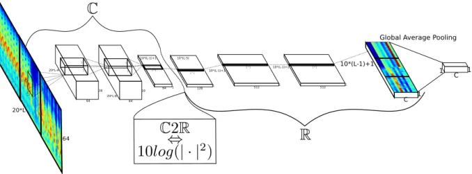
Figure 1: Illustration of the proposed partially complex CRNet architecture. The first1D convolutional layer is
omitted, as well as activations and normalization layers, and the real-valued spectrogram is shown for visual clarity, although the complex spectrogram serves as true input.
more parameters, but may also suffer from overfitting when a sufficient amount of diversified data is not met. A reasonable way to experiment on this interrogation is to allow half as many channels in the CRNet’S convolutional blocks and focussing experiments on small amounts
of data. Results show that keeping the same number of channels as in the real network still performs better, which is a conclusive statement as, while the practical number of parameters has doubled, the network did not suffer even when presented with few data. As a sanity check, doubling the number of channels in the complex network performs the worst of all cases.
Signal scaling and complex representation Raw radar data, along with their Fourier transforms, often exhibit major variations in scale, due to different intervening physical phenomena oper-ating in a variety of scales. This translates to the practical habit of converting spectrograms to a logarithmic scale, most often decibels, whether it be for visualization or further analysis. A real-valued network benefits from this rescaling from the start as the inputs are the decibel-spectrograms. In theCRNet however, the log-scale is ambiguously defined for complex values, which allows potentially harmful variations in scale to propagate within. Proper weight initial-ization and batchnorm explicitly combat this issue, but formally fail to recover a log-scale as they remain linear transformations. To this end, we propose a partially complex network for which the output complex representation is log-scaled after the passage to absolute value, and heuristically study the impact on performance of the complex-to-real (C2R(x) = 10log(|x|2|)) function’s position in the layer hierarchy. The conclusion is conceptually satisfying as it places theC2Rright after the final temporal representation layer, ie right before the convolutionalized fully-connected layers [6], as represented in figure 1; in practice the ante-penultimate convolu-tional layer of the network proposed in [3]. This result leads to a rather natural interpretation: while the complex spectral representation of the signal in a real-valued network stops at the Fourier transform, the latter in aCRNet explores a hierarchy of further filter banks in addition
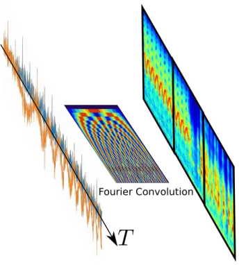
Fourier Convolution
Figure 2: Illustration of the proposed Fourier-like convolutional layer. The Fourier atoms are represented as sine waves of increasing frequency.
to the Fourier filtering.
Fourier convolution parameters The first layer of a CNN on spectrograms is conceptually pre-ceded by a windowed Fourier transform, which remains a fixed pre-processing. The CRNet however directly handles the raw complex data, and as such, its first layer is a1D convolution. While conventional initialization schemes such as [7] can be applied, we may benefit from ex-ploiting the spectral properties of the radar signal. Indeed, since the Fourier transform is essen-tially a convolution, we can initialize the filter bank weights to thenFourier atoms(e−2iπkn·)k≤n,
wheren represents the windowing applied to the signal, and corresponds to the 1D filter size; such a layer is represented in figure 2. Experiments show a consistent improvement when using such a Fourier-like convolutional layer. Similarly, the window overlap percentage or hop length of the Fourier transform corresponds to the convolution stride. In the context of learning the1D filter banks, a low stride (set to1in the experiments, ie maximum overlap) proved paramount to the network’s performance, regardless of initialization. On the other hand, real-valued counter-parts seemed much more robust to this hyperparameter. One interpretation of this phenomenon is that the passage from raw complex data to real-valued spectrograms averages through co-herent integration any potential added information from a higher overlap, while keeping both amplitude and phase sensitizes further processing to this added information. We call FourierNet aCRwhose first convolutional layer is initialized with the Fourier atoms.
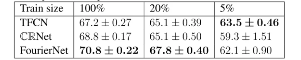
Table 1: Performance comparison of complex and real networks on radar data on various amount of noisy data.
Train size 100% 20% 5%
TFCN 67.2±0.27 65.1±0.39 63.5±0.46
CRNet 68.8±0.17 65.1±0.50 59.3±1.51
FourierNet 70.8±0.22 67.8±0.40 62.1±0.90
Quality and amount of data Throughout conducted experiments, a general trend seemed to
emerge: complex networks overpowered real networks when presented with a large yet compli-cated dataset. Specifically, we observed improvement forSN Rs on the IQ data close to zero or in the negatives, positiveSN Rs leading to insignificant improvements. Furthermore, when the amount of training data was kept relatively small (in our scenario, less than5minutes),CRNets performed poorly to worse than their real-valued counterpart.
4.2. Results
In this section we show experimental results on synthetic radar data, issued by the simulator in-troduced in [3]. Approximately20minutes of signal are generated for each of3different classes of drones; signals are passed through the models35ms at a time. The simulation configurations are set to an extremely noisy case, where the raw data is5dB below noise (SN R=−5dB). For reference, a coherent integration of20timesteps (which corresponds to the filter size of the first convolutional layer) would bring the spectrum8dBabove noise. A PRF of4kHzis used; at this frequency and with the considered drones, Doppler ambiguity is omnipresent. As stated above, we voluntarily chose a large amount of data in a very challenging configuration. We also give performance results for the models when trained on a fraction of the data to quantify the robust-ness of the models to lack of data. All models are run in a 5-fold cross-validation, holding out
50%of data for validation, using standard gradient descent. Three models are put to testing: the real-valued TFCN, the corresponding CRNet and the equivalent FourierNet. The architectural
choices described above are included in the complex models. Results are presented in table 1. The first observation is the improvement of the two complex networks over the real counterpart when given all 10minutes of training data (the50% training split of the total20minutes), the FourierNet being superior to theCRNet. Given20% of available training data (2minutes), the FourierNet still outperforms all models, but the CRNet starts decreasing towards the TFCN’s performance. Given only5% of training data (30seconds), all complex models begin to perform worse than the TFCN. Finally, we repeat the experiments on a cleaner dataset, by changing the
SN R from−5dB to5dB (we limit ourselves to the FTCN and FourierNet). Results shown in table 2 naturally exhibit better performances overall, but the FourierNet struggles to outperform the FTCN, which supports the argument of complex networks working noticeably better in challenging configurations only.
Table 2: Performance comparison of complex and real networks on radar data on various amount of less noisy data.
Train size 100% 20% 5%
TFCN 98.6±0.34 94.3±0.57 91.6±0.98
FourierNet 99.0±0.07 94.4±0.14 88.7±1.12
5. Conclusion
In conclusion, we have developed a fully-temporal, partially-complex convolutional neural net-work combining previous net-works on complex-valued neural netnet-works on the one hand, and fully-temporal networks for radar classification on the other hand. We have furthermore introduced a Fourier-like convolutional layer, which harvests the advantages of both the Fourier trans-form and of learning filter banks on the raw data, an intuition proved to be consistently true in practice. We performed extensive experimentation on synthetic data to isolate the cases where performance benefitted from complex values. The main conclusions obtained were, that above a certain amount of observed data (a couple of minutes for our datasets), in challenging config-urations (under5dB ofSN Rin our scenarios), complex-valued networks significantly outper-formed their real counterparts. These results initiate a hopeful stance on introducing complex values in deep learning-based classification methods on micro-Doppler radar data.
References
[1] A. v. d. Bos. Complex gradient and Hessian. IEE Proceedings - Vision, Image and Signal Process-ing, 141(6):380–383, Dec. 1994.
[2] D. H. Brandwood. A complex gradient operator and its application in adaptive array theory. IEE Proceedings H - Microwaves, Optics and Antennas, 130(1):11–16, Feb. 1983.
[3] D. A. Brooks, O. Schwander, F. Barbaresco, J. Schneider, and M. Cord. Temporal Deep Learning for Drone Micro-Doppler Classification. In2018 19th International Radar Symposium (IRS), pages 1–10, June 2018.
[4] V. C. Chen, F. Li, S.-S. Ho, and H. Wechsler. Micro-Doppler effect in radar: phenomenon, model, and simulation study. IEEE Transactions on Aerospace and electronic systems, 42(1):2–21, 2006. [5] J. J. M. De Wit, R. I. A. Harmanny, and P. Molchanov. Radar micro-Doppler feature extraction
using the singular value decomposition. InRadar Conference (Radar), 2014 International, pages 1–6. IEEE, 2014.
[6] R. Girshick. Fast R-CNN. arXiv:1504.08083 [cs], Apr. 2015. arXiv: 1504.08083.
[7] X. Glorot and Y. Bengio. Understanding the difficulty of training deep feedforward neural net-works. In Proceedings of the Thirteenth International Conference on Artificial Intelligence and Statistics, pages 249–256, Mar. 2010.
[8] S. Ioffe and C. Szegedy. Batch Normalization: Accelerating Deep Network Training by Reducing Internal Covariate Shift. arXiv:1502.03167 [cs], Feb. 2015. arXiv: 1502.03167.
[9] P. Molchanov, R. I. Harmanny, J. J. de Wit, K. Egiazarian, and J. Astola. Classification of small UAVs and birds by micro-Doppler signatures. International Journal of Microwave and Wireless Technologies, 6(3-4):435–444, June 2014.
[10] C. Trabelsi, O. Bilaniuk, Y. Zhang, D. Serdyuk, S. Subramanian, J. F. Santos, S. Mehri, N. Ros-tamzadeh, Y. Bengio, and C. J. Pal. Deep Complex Networks. arXiv:1705.09792 [cs], May 2017. arXiv: 1705.09792.
[11] R. P. Trommel, R. I. A. Harmanny, L. Cifola, and J. N. Driessen. Multi-target human gait classifica-tion using deep convoluclassifica-tional neural networks on micro-doppler spectrograms. In2016 European Radar Conference (EuRAD), pages 81–84, Oct. 2016.
[12] W. Wirtinger. Zur formalen Theorie der Funktionen von mehr komplexen Vernderlichen. Mathe-matische Annalen, 97(1):357–375, Dec. 1927.
[13] B. Xu, N. Wang, T. Chen, and M. Li. Empirical Evaluation of Rectified Activations in Convolu-tional Network. arXiv:1505.00853 [cs, stat], May 2015. arXiv: 1505.00853.