Diversity Assessment of Multi-Objective Evolutionary
Algorithms: Performance Metric and Benchmark Problems
Ye Tian, Institutes of Physical Science and Information Technology, Anhui University, Hefei, China
Ran Cheng, Shenzhen Key Laboratory of Computational Intelligence, University Key Laboratory of Evolving
Intelligent Systems of Guangdong Province, Department of Computer Science and Engineering, Southern
University of Science and Technology, Shenzhen, China
Xingyi Zhang, School of Computer Science and Technology, Anhui University, Hefei, China; State Key
Laboratory of Synthetical Automation for Process Industries, Northeastern University, Shenyang, China
Miqing Li, School of Computer Science, University of Birmingham, Birmingham, U.K.
Yaochu Jin, Department of Computer Science, University of Surrey, Guildford, U.K.
Abstract—Diversity preservation plays an important role in the design of multi-objective evolutionary algorithms, but the diversity performance assessment of these algorithms remains challenging. To address this issue, this paper proposes a per-formance metric and a multi-objective test suite for the diver-sity assessment of multi-objective evolutionary algorithms. The proposed metric assesses both the evenness and spread of a solution set by projecting it to a lower-dimensional hypercube and calculating the “volume” of the projected solution set. The proposed test suite contains eight benchmark problems, which pose stiff challenges for existing algorithms to obtain a diverse solution set. Experimental studies demonstrate that the proposed metric can assess the diversity of a solution set more precisely than existing ones, and the proposed test suite can be used to effectively distinguish between algorithms with respect to their diversity performance.
I. INTRODUCTION
During the last two decades, multi-objective evolutionary algorithms (MOEAs) have attracted an increasing interest in the evolutionary computation community [1]. An important reason for the prevalence of MOEAs is that they can obtain a set of solutions for a multi-objective optimization problem (MOP) in a single run, where the quality of a solution set is usually evaluated from three aspects, namely, convergence, evenness, and spread. The evenness and spread are also collectively known as the diversity. Note that in this paper, we focus on these properties of a solution set in the objective space rather than in the decision space, in spite of the equal importance of the latter one [2].
While many MOEAs aim at enhancing the convergence of a solution set [3], [4], there has been an increasing number of MOEAs focusing on preserving the diversity of a solution set in recent years, such as the diversity estimation based MOEAs [5], [6], the decomposition based MOEAs [7], [8], and the indicator based MOEAs [9], [10]. Diversity preservation is an important topic in MOEAs, since a solution set with better diversity can provide decision makers more information when Supplementary materials of this paper are available at https://www.researchgate.net/publication/332406734, source codes of CPF and IMOP1–IMOP8 have been embedded in PlatEMO and are available at https://github.com/BIMK/PlatEMO.
Corresponding Author: Xingyi Zhang (E-mail: [email protected])
f f o 3DUHWRIURQW *RRGHYHQQHVV SRRUVSUHDG 6ROXWLRQV
(a) Solution setS1
f f o 3DUHWRIURQW 3RRUHYHQQHVV JRRGVSUHDG 6ROXWLRQV (b) Solution setS2 f f o 3DUHWRIURQW *RRGHYHQQHVV JRRGVSUHDG 6ROXWLRQV (c) Solution setS3
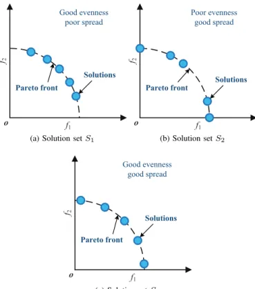
Fig. 1. Three solution sets for a bi-objective optimization problem. choosing their preferred solutions [11]. Moreover, some real-world applications naturally require a solution set with good diversity. For example, ensemble learning requires multiple models with sufficient differences [12].
Due to the importance of diversity in the obtained solution sets, some metrics have been designed for assessing the diversity performance of MOEAs, which can be divided into two categories, i.e., metrics assessing only diversity and met-rics assessing both convergence and diversity. However, most of these metrics have limitations. For the metrics assessing only diversity, some of them (e.g., Spacing [13]) bias the assessment of evenness, and some others (e.g., CLµ [14])
bias the assessment of spread, whereas few of them are able to assess both the evenness and spread of a solution set. Consider the three solution sets depicted in Fig. 1, where S1 has a
good evenness and a poor spread, S2 has a poor evenness
and a good spread, and S3 has a good evenness and a good
spread. Obviously, the diversity of S3 is significantly better
than S1 and S2. However, for the diversity metrics biasing
the assessment of evenness, they may identify S1 as the one
with the best diversity; similarly, the metrics biasing towards the assessment of spread may identify S2 as the one with the
best diversity. As for the metrics assessing both convergence and diversity (e.g., IGD [15]), it is difficult to merely assess diversity without considering convergence.
To address this issue, this paper proposes a new diversity metric that can effectively assess both the evenness and spread of a solution set obtained by MOEAs. To better compare the diversity performance of different MOEAs, this paper also proposes a multi-objective test suite containing various complex Pareto fronts, which poses stiff challenges for existing MOEAs in terms of diversity preservation. Specifically, the contributions of this paper consist of the following two aspects: • A performance metric is proposed for assessing the diversity of a solution set obtained by MOEAs. The proposed metric assesses both the evenness and spread of a solution set by projecting it to the (M − 1) -dimensional unit hypercube (M denotes the number of objectives), and calculating the “volume” of the projected solution set as its diversity. Both illustrative examples and experimental studies indicate that the proposed metric has better performance in diversity assessment than existing metrics.
• A multi-objective test suite is proposed for comparing the diversity performance of existing MOEAs, which contains eight bi- or three-objective MOPs with simple landscapes but various irregular Pareto fronts. The pro-posed test suite poses stiff challenges to existing MOEAs to obtain a set of solutions with good evenness and spread, thereby effectively distinguishing between the diversity performance of different MOEAs. According to the experimental results of five popular MOEAs on the proposed test suite, it turns out that the compared MOEAs exhibit significantly different diversity performance, and none of them is able to perform consistently well on all the proposed MOPs.
The rest of this paper is organized as follows. In Section II, existing metrics for diversity assessment are revisited and the proposed metric is detailed. In Section III, the effectiveness of the proposed metric is verified by comparing it with several metrics in assessing the diversity of solution sets obtained by five popular MOEAs. In Section IV, existing multi-objective test suites are reviewed, followed by a description of the proposed test suite and the performance verification. Finally, conclusions are drawn in Section V.
II. PROPOSEDMETRIC FORDIVERSITYASSESSMENT
A. Existing Metrics for Diversity Assessment
In general, the performance metrics in multi-objective opti-mization can be divided into those assessing only convergence (e.g., GD [16] and CM [17]), those assessing only diversity (e.g., Spacing [13] and PD [11]), and those assessing both
convergence and diversity (e.g., IGD [15] and HV [18]). A detailed list of most existing performance metrics can be found in [19]. In the following, we review the metrics assessing only diversity, which can be further grouped into three categories. The first category of metrics assesses the diversity by calculating the minimum Euclidean distance of each solution to the others in the solution set, such as Spacing [13] and∆
[20]. For example, the Spacing value of a solution setP can be calculated by Spacing(P) = v u u t 1 |P| −1 |P| ∑ i=1 (d−di)2, (1)
where di denotes the minimum distance of thei-th solution
to the others inP, andddenotes the mean of alldi. In short,
Spacing measures the standard deviation of the minimum distances of each solution to the others. Hence, this metric assesses the evenness of a solution set without considering its spread.
The second category assesses the diversity by dividing the objective space into grids and counting the grids having at least one solution, such asCLµ[14], DM [17], and DCI [19].
For example,CLµ divides the solutions in P into a number
of hypercubes and assesses the diversity ofP by
CLµ(P) = |P| N DCµ(P)
, (2)
whereN DCµ(P)is the number of hypercubes having at least
one solution, and µ is a parameter denoting the number of divisions on each objective. Obviously,CLµ mainly assesses
the spread of a solution set, since it does not consider the evenness of solutions within the same hypercube. Besides, according to (2), a solution set containing fewer solutions may have better (i.e., smaller) CLµ value.
The third category adopts the measures in other fields, such as experimental design [21], spatial informatics [22], and biology [23]. Taking the PD [11] used for measuring the biodiversity as an example, it calculates the diversity of a solution setP by
P D(P) = max
p∈P(P D(P\ {p}) +q∈minP\{p}∥f(p)−f(q)∥p),
(3) where ∥f(p)−f(q)∥p denotes the Lp-norm based distance
between solutions p and q in objective space. It should be noted that PD is designed for assessing the diversity of points filling a hypercube, whereas the Pareto optimal solutions for an MOP usually lie on an (M −1)-dimensional manifold in an M-dimensional objective space [24], so that the solutions far away from the Pareto front usually contribute more to the PD value. As a consequence, PD mainly considers the spread since the solutions with worse convergence usually have larger spread.
It is worth noting that the metrics assessing both conver-gence and diversity can also be used to distinguish between the diversity of two solution sets if they have similar convergence, such as IGD [15],∆p [25], and HV [18]. A set of reference
points uniformly sampled on the Pareto front is required for the calculation of IGD and ∆p, where IGD calculates the
0 0 0.5 f3 1 f 1 0.5 1 f 2 0.5 1 0
(a) Solution setP1
0 0 0.5 f3 1 f 1 0.5 1 f 2 0.5 1 0 (b) Solution setP2 0 0 0.5 f3 1 f 1 0.5 1 f 2 0.5 1 0 (c) Solution setP3 0 0 0.5 f 3 1 f 1 0.5 1 f 2 0.5 1 0 (d) Solution setP4
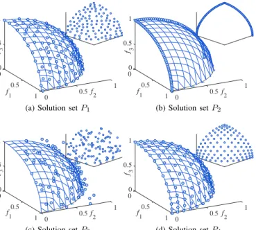
Fig. 2. Four solution sets with different distributions. The Pareto front is assumed to be a unit sphere in the first octant. Note that the diversity ofP4
is worse thanP1since the solutions on the border ofP4are more crowded
than those in the middle.
averaged minimum distance between each reference point and the solution set and ∆p calculates the averaged Hausdorff
distance between the reference point set and the solution set. Besides, a reference point is required for the HV metric to calculate the hypervolume of the area covered by a solution set with respect to it. It is worth noting that the reference point for the HV calculation is an anti-optimal point, which is different from the reference points used for the calculation of IGD or ∆p.
B. Limitations of Existing Metrics in Diversity Assessment
To illustrate the limitations of existing metrics in diversity assessment, we consider four solution sets shown in Fig. 2 with different distributions, where each set consists of 105 non-dominated solutions. The Pareto front is assumed to be a unit sphere in the first octant. It is clear that P1 has good
evenness and spread, whereasP2 merely concentrates on two
curves of the Pareto front, and most solutions in P3 do not
converge to the Pareto front.P4 is obtained by projecting the
solutions sampled by Das and Dennis’s method [26] to the unit sphere. Note that the spread of P4 is similar to P1, but
the evenness ofP4is worse thanP1since the solutions on the
border of P4 are obviously more crowded than those in the
middle.
In this example, Spacing, CLµ, PD, IGD,∆p, and HV are
employed to assess the diversity of the four solution sets. As suggested in the literature [7], [27], the reference points for calculating IGD and∆pare 9870 points obtained by the same
method asP4. Besides, the parameterµinCLµ is set to 10,
the parameter p in PD is set to 0.1, the parameter p in ∆p
is set to 2, and the reference point for calculating HV is set to (1.1,1.1,1.1). Note that smaller values of Spacing, CLµ,
IGD, and∆p and larger values of PD and HV indicate better
diversity.
TABLE I
THESPACING,CLµ, PD, IGD,∆p,ANDHV VALUES OF THEFOUR
SOLUTIONSETSSHOWN INFIG. 2. THEBESTMETRICVALUE INEACH
ROW ISHIGHLIGHTED.
Metric P1 P2 P3 P4
Spacing 2.4167e-2 4.4648e-3 5.6212e-2 5.2543e-2
CLµ 2.6923e+0 8.0769e+0 2.3864e+0 2.6923e+0
PD 1.8698e+5 2.9967e+3 2.0248e+5 6.0207e+4 IGD 5.1811e-2 2.5648e-1 9.1023e-2 5.0300e-2
∆p 5.1811e-2 2.5648e-1 9.1023e-2 5.0300e-2
HV 7.4797e-1 6.5432e-1 6.4469e-1 7.4938e-1
As shown in Table I, none of the metrics identifies P1 as
the one with the best diversity, despite that P1 has the best
diversity among the four solution sets. To be specific, Spacing merely calculates the standard deviation of the minimum distances between each solution and the others. Since the solutions inP2have smaller distances to each other than those
in the other solution sets,P2has the best Spacing value.CLµ
and PD consider spread much more important than evenness, soP3obtains the bestCLµand PD values. Since the reference
points for the IGD calculation and the solutions in P4 have
the same distribution, P4 has a better IGD value than the
other solution sets. In fact,P1andP4have similar spread, but
according to the Spacing values ofP1andP4, i.e., the standard
deviations of the minimum distances between solutions, the evenness of P1 is much better thanP4. Due to the relatively
good convergence of the four solution sets, the metric∆pwith p= 2 is equivalent to IGD [25], so that P4 has the best∆p
value as well. Lastly,P4 also has a better HV value than P1,
since the HV contributions of the solutions on the borders of concave surfaces (e.g., a sphere) become larger than those on the borders of convex surfaces, which leads the HV metric to present that bias.
To summarize, none of the six metrics makesP1obtain the
best diversity due to various limitations. Specifically, Spacing makesP2 have the best diversity since it merely assesses the
evenness of each solution set.CLµ and PD makeP3 achieve
the best diversity as they mainly emphasize on the spread. IGD and∆p enableP4to have the best evaluation result due to the
same distribution of the reference points toP4. And P4 also
has the largest HV value since it contains a large proportion of solutions nearby the border of a concave surface, which are biased by the metric. In order to overcome the limitations of these existing metrics, a diversity metric that can assess both the evenness and spread of a given solution set is proposed in the following.
C. The Proposed Diversity Metric
The main idea of the proposed metric is to project a solution set in an M-dimensional objective space to an (M −1) -dimensional space, and then assess the diversity of the pro-jected solution set. Such a projection has two advantages: First, since a solution set usually lies on an (M −1)-dimensional manifold in anM-dimensional objective space, there does not exist any solution in most area of the objective space. By contrast, the projected solution set fills an(M−1)-dimensional hypercube in an(M−1)-dimensional space, hence it is easier to assess the diversity in such a sufficiently sampled space.
Second, the projection eliminates the influence of convergence performance. As shown in Table I,CLµand PD makeP3have
the best diversity since the convergence of P3 is significantly
worse than the other solution sets, which means that the diversity assessment has been influenced by the convergence of the solution sets.
The proposed metric, termed coverage over the Pareto front (CPF), defines the diversity of a solution set as its coverage over the Pareto front in an (M −1)-dimensional hypercube. To begin with, the CPF projects all the solutions to the Pareto front to eliminate the effect of convergence performance. Since it is difficult to calculate the foot point of each solution on a complex Pareto front, a large number of reference points are sampled on the Pareto front, and each solution is replaced by its closest reference point. Thus, a new point set P′ can be constructed by
P′={argminr∈R∥r−f(x)∥ |x∈P}, (4)
where R denotes the set of reference points sampled on the Pareto front, P denotes the set of solutions to be assessed, and∥r−f(x)∥ denotes the Euclidean distance between point rand solutionxin objective space. Obviously,P′ is a subset ofR. Then each pointpinP′ andRis normalized according to the minimum and maximum objective values in R, i.e.,
pi=
pi−minr∈Rri maxr∈Rri−minr∈Rri
, fori= 1, . . . , M, (5) where pi denotes thei-th objective value of pandM is the
number of objectives. Afterwards, all the points inP′ andR
are projected to a unit simplex by the following three steps, i.e., projection, translation, and normalization:
1) For each pointpinP′andR,pi=pi+M1 −M1
∑M
j=1pj, i= 1, . . . , M;
2) For each point p in P′ and R, pi = pi−minr∈Rri, i= 1, . . . , M;
3) For each point pinP′ andR,pi =pi/
∑M
j=1pj,i= 1, . . . , M.
In this way, all the points in P′ and R are located on the unit simplex f1+. . .+fM = 1 and within [0,1]M. Taking
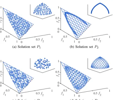
the solution sets shown in Fig. 2 as an example, the solution sets after being projected to the unit simplex are presented in Fig. 3, where the reference point set R is the same to that used in the IGD calculation in Table I.
It is worth noting that some MOEAs also assess the diversity by projecting the solutions to a simplex [28], [29], but these methods are different from that in the proposed CPF. Specifi-cally, the proposed CPF projects each pointpto its foot drawn to the simplex, whereas those MOEAs project each point p to the intersection of −→op and the simplex. In this way, the projection method in CPF fixes the parallel distances between points, whereas the projection method in existing MOEAs fixes the angles between points. As shown in Fig. 4, the points projected by CPF have a similar distribution to the original points; by contrast, the distribution of the points is highly distorted after being projected by existing MOEAs, where the points in the middle of the simplex become more crowded than those on the border. As illustration, Table II lists the Spacing values of the four solution sets shown in Fig. 2 as well as
0 0 0.5 f3 1 f 1 0.5 1 f 2 0.5 1 0
(a) Solution setP1
0 0 0.5 f3 1 f 1 0.5 1 f 2 0.5 1 0 (b) Solution setP2 0 0 0.5 f 3 1 f 1 0.5 1 f 2 0.5 1 0 (c) Solution setP3 0 0 0.5 f3 1 f 1 0.5 1 f 2 0.5 1 0 (d) Solution setP4
Fig. 3. The four solution sets given in Fig. 2 after being projected to a unit simplex. f f o 2ULJLQDOSRLQWV 3URMHFWHGSRLQWV (a) CPF f f o 2ULJLQDOSRLQWV 3URMHFWHGSRLQWV (b) Existing MOEAs Fig. 4. The projection methods in CPF and some existing MOEAs. those projected by the methods in CPF and existing MOEAs. It can be seen that P2 has the best evenness (i.e., smallest
Spacing value), which is followed by P1, P4 and P3. After
being projected by CPF, the rank of the four solution sets in terms of Spacing is not changed. But if the solution sets are projected by existing MOEAs,P4 and P1 will have the best
and the worst evenness, respectively. Therefore, the projection method in CPF can effectively reduce this distortion.
After projecting the points in P′ and R to the (M −1) -dimensional unit simplex in an M-dimensional objective space, they are further projected to an (M −1)-dimensional unit hypercube in an (M −1)-dimensional space, which is achieved by the mixture uniform design [21]. To be specific, for each projected point p′ = (p′1, . . . , p′M−1), the point p= (p1, . . . , pM)can be calculated by { pi= [1−(p′i) 1 M−i]∏i−1 j=1(p′j) 1 M−j, 1≤i < M pi= ∏i−1 j=1(p′j) 1 M−j, i=M . (6)
Therefore, we can obtain the point p′ in an (M − 1) -dimensional space by solving the above equations according to each pointp∈P′∪Rthat is in anM-dimensional objective space.
TABLE II
THESPACINGVALUES OF THEFOURSOLUTIONSETSSHOWN INFIG. 2
ANDTHOSEPROJECTED BY THEMETHODS INCPFANDEXISTING
MOEAS. Projection
P1 P2 P3 P4 Ascending
method order
Original 2.42e-2 4.46e-3 5.62e-2 5.25e-2 P2, P1, P4, P3
CPF 1.46e-2 2.56e-3 3.25e-2 2.65e-2 P2, P1, P4, P3
Existing
3.48e-2 8.37e-3 3.45e-2 7.71e-7 P4, P2, P3, P1
MOEAs
After the projection of the points inP′ andR, the diversity of the projected point setP′ is assessed as the diversity of the original solution set P. In the proposed CPF, the diversity is defined as the coverage ofP′ over the reference point set R, i.e., the ratio of the “volume” ofP′ to the “volume” ofR. To this end, the monopolized hypercube is defined on each point in P′ and R, which measures the “volume” of a point set by considering both evenness and spread. The monopolized hypercube of each point p in P′ is defined as a hypercube centered at p, where the side length lp of the monopolized hypercube is obtained by
lp= min
q∈P′\{p}i=1max,...,M−1|pi−qi|. (7)
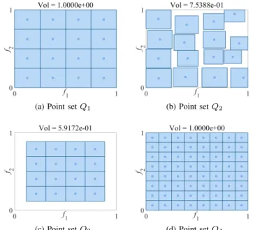
Consequently, each monopolized hypercube never intersects the others, and it can have a side length as large as possible. Fig. 5 plots the monopolized hypercubes of the points in four sets, where three properties of the monopolized hypercube can be observed from the figure:
• As shown in Fig. 5 (a), the monopolized hypercubes of all the points do not intersect each other, and the “volume” of the point set P′ is defined as the summation of the volumes of all the monopolized hypercubes, i.e.,
V ol(P′) = ∑ p∈P′
lMp−1. (8)
In particular, a point set with perfect diversity has the maximum “volume” of 1.
• As shown in Fig. 5 (b) and (c), the point set with either poor evenness or poor spread has a small “volume”, hence it considers both the evenness and spread of the point set. • As shown in Fig. 5 (a) and (d), the “volume” is indepen-dent of the number of points, so the diversity of two point sets with different sizes is comparable. This property is very important to CPF since it calculates the ratio of the “volume” of the projected point set P′ to the “volume” of the reference point set R, where R is usually much larger thanP′.
Note that the outliers in P′ may have extremely large monopolized hypercubes, hence the side length lp of each pointpinP′ is further restricted by
lp= min{lp,(V ol(R) |P′| )
1
M−1}. (9)
In this way, the “volume” of P′ will be always smaller than or equal to the “volume” of R. Besides, the monopolized hypercubes of extreme points in P′ and R should be further shrunk to make them always located inside the unit hypercube,
(a) Point setQ1 (b) Point setQ2
(c) Point setQ3 (d) Point setQ4
Fig. 5. The monopolized hypercubes (shown in gray regions) of the points in four sets, where the “volume” (i.e., diversity) of each point set is defined as the summation of the volumes of all the monopolized hypercubes.
(a) Solution setP1 (b) Solution setP2
(c) Solution setP3 (d) Solution setP4
Fig. 6. The monopolized hypercubes of the solutions given in Fig. 2, where the “volume” (i.e., diversity) of each solution set is defined as the summation of the volumes of all the monopolized hypercubes.
i.e.,
lpi = min(1, pi+lp/2)−max(0, pi−lp/2), (10)
wherelpi denotes the size length ofpin thei-th dimension. In
this case, the monopolized hypercube of a point is no longer centered at the point.
Considering the four solution sets given in Fig. 2, the monopolized hypercubes of the solutions in these sets are shown in Fig. 6, where the “volumes” ofP1,P2,P3andP4are
3.9703e-1, 4.9094e-2, 2.0352e-1 and 3.8653e-1, respectively. Besides, the reference point set has a “volume” of 5.4996e-1. Therefore, the CPF values of the four solution sets, i.e., the ratios of the “volumes” of the four solution sets to the
Algorithm 1: Procedure of the proposed CPF
Input:P (solution set),R (reference point set)
Output:CP F (CPF value ofP)
1 P′← Replace each solution inP by its closest reference
point inR;
2 Normalize the points in P′ andRby (5); 3 Project the points in P′ andR to a unit simplex; 4 Project the points in P′ andR to a unit hypercube; 5 Calculate the side length of each monopolized hypercube
inR by (7);
6 Shrink the size length of each monopolized hypercube in
R by (10);
7 V ol(R)←Calculate the “volume” ofRby (8);
8 Calculate the side length of each monopolized hypercube
inP′ by (7);
9 Restrict the side length of each monopolized hypercube
inP′ by (9);
10 Shrink the size length of each monopolized hypercube in
P′ by (10);
11 V ol(P′)←Calculate the “volume” ofP′ by (8); 12 CP F ←V ol(P′)/V ol(R);
“volume” of the reference point set, are 7.2193e-1, 8.9269e-2, 3.7006e-1 and 7.0283e-1, respectively, where the CPF value of P1 is better than the others and thus correctly reflects the
diversity of the four solution sets. It is worth noting that the CPF value of any solution set is within [0,1] and not monotonic with the number of solutions, which means that a solution set to which some solution have been added may have smaller CPF value than the same solution set without the additional solutions. Therefore, if the density of the solution set is considered as an important property, an additional metric should be adopted to take it into account.
Algorithm 1 summarizes the procedure of the proposed CPF. As can be seen, the time complexity of CPF is mainly determined by the calculation of the “volume” of R, since there are a much larger number of points in R than in P. According to (7), the time complexity of CPF is O(M N2),
whereM andNdenote the number of objectives and reference points in R, respectively.
D. Similarity and Difference Between CPF and Other Metrics
1) CPF vs. Spacing: Spacing calculates the distances
be-tween solutions, which can only assess the evenness of a solution set. By contrast, the proposed CPF calculates the “volume” of a solution set, which can assess both evenness and spread.
2) CPF vs. CLµ: Both CLµ and CPF are based on a
number of hypercubes. However, the CLµcounts the number
of hypercubes having at least one solution, which mainly assesses the spread of a solution set. Moreover, according to the definition of CLµ, a solution set with fewer solutions
may have a better metric value. By contrast, due to the third property of monopolized hypercube, the diversity of two solution sets with different sizes is comparable when using CPF.
(a)P D= 2.6667e+0 (b)P D= 2.4236e+2 Fig. 7. Two solution sets with different distributions. The “volume” of the left set is larger than the “volume” of the right set, but the PD value of the left set is much worse than the PD value of the right set.
3) CPF vs. PD: Both PD and the monopolized hypercube
in CPF are designed for assessing the diversity of a point set filling in a unit hypercube. As mentioned before, the diversity assessment in PD may be influenced by the convergence of a solution set, whereas CPF can eliminate such an influence by projecting the solution set to a lower-dimensional space. In addition, as illustrated by the example shown in Fig. 7, even for two solution sets with similar convergence, PD may misjudge their diversity due to the outlier in the solution set. In contrast to PD, the monopolized hypercube is not influenced by the outlier due to the restriction of the size length.
4) CPF vs. IGD & ∆p: IGD, ∆p, and CPF require a set
of reference points sampled on the Pareto front to work. As mentioned before, the diversity assessment in IGD and∆p is
sensitive to the distribution of the reference point set, since they determine the closest solution of each reference point. By contrast, since the proposed CPF is similar to GD [16] that projects solutions to the Pareto front by finding the foot point of each solution, more reference points can lead to a more accurate projection, where the reference points do not need to have an even distribution.
5) CPF vs. HV: As mentioned before, since the HV
contributions of the solutions on the borders of concave surfaces become larger than those on the centers, a solution set with more/fewer crowded solutions on the borders of concave/convex surfaces may obtain a larger HV value than a solution set with even distribution. By contrast, the proposed CPF projects the solution set to a unit simplex in advance, such that it is not influenced by the curvature of the solution set.
Since Spacing, CLµ, PD, and HV do not require a set of
reference points sampled on the Pareto front, they are able to assess the diversity of solutions for real-world MOPs whose Pareto fronts are unknown. By contrast, IGD and ∆p cannot
work without a set of reference points. It is worth noting that the proposed CPF can also assess the diversity of solutions without any reference point. In this case, CPF first projects the solutions to an (M −1)-dimensional unit simplex, such that the effect of convergence can be eliminated. Then it projects the solutions to an(M −1)-dimensional unit hypercube and calculates the “volume” of the projected solutions as the metric value. As a consequence, the proposed CPF can also be applied to real-world MOPs by performing Steps 3, 4, 8, 10, and 11 in Algorithm 1.
III. EXPERIMENTALRESULTS ON THEPROPOSEDMETRIC In order to verify the effectiveness of the proposed CPF in diversity assessment, five selected MOEAs are investigated on the DTLZ test suite [30], and the experimental results are analyzed by several diversity metrics including the proposed CPF. We also consider a real-world problem CWDV (i.e., crash-worthiness design of vehicles for complete trade-off front) [31] to verify the effectiveness of CPF without any reference point, and a many-objective optimization problem ML-DMP (i.e., multi-line distance minimization problem) [32] to verify the effectiveness of CPF in high-dimensional space. All the experiments are implemented on PlatEMO [33].
A. MOEAs under Comparison
Five promising MOEAs are involved in the experiments, namely, SPEA2 [34], IBEA [35], NSGA-III [7], BCE-IBEA [36], and SMS-EMOA [37], most of which have been demon-strated to exhibit a good diversity performance on benchmark MOPs. A brief introduction to the five MOEAs is given in the following.
1) SPEA2 uses the truncation method as the main strategy in environmental selection, which can obtain a popu-lation with good diversity. Although SPEA2 has been published for more than ten years, it is one of the most effective MOEAs in diversity preservation so far. 2) IBEA is one of the representative indicator based
MOEAs. It defines the optimization goal in terms of a binary indicator and then directly uses this indicator in environmental selection. Since the indicator considers both convergence and diversity, IBEA is expected to obtain a population with good convergence and diversity. 3) NSGA-III first sorts the solutions by non-dominated sorting [38], then selects one solution for each reference point. By adopting the advantages of both Pareto dom-inance based MOEA and decomposition based MOEA, NSGA-III shows competitive performance on many MOPs.
4) BCE-IBEA embeds the Pareto criterion in IBEA by an external archive storing well-distributed non-dominated solutions obtained during the evolution process. It was evidenced that the population obtained by BCE-IBEA has much better diversity than that obtained by IBEA. 5) SMS-EMOA is an MOEA based on HV. It is a
steady-state algorithm that generates one new solution at each generation, then the solution with the least contribution to the HV of the population is replaced with the newly generated one. By doing so, it is expected to obtain a population with a good HV value.
The optimal parameter settings of the compared MOEAs are adopted. Specifically, the fitness scaling factor in IBEA and BCE-IBEA is set to 0.0001 for DTLZ1 and DTLZ3, and 0.005 for the remaining MOPs. The population size N
of all the compared MOEAs is set to 100, 105, and 156 for the MOPs with two, three, and eight objectives, respectively. The maximum number of generations is set to 300, which is enough for the MOEAs to converge. As for the genetic operators, all the compared MOEAs adopt simulated binary
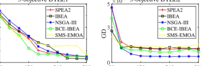
30 120 210 300 Generations 10-4 10-1 101 GD 3-objective DTLZ1 SPEA2 IBEA NSGA-III BCE-IBEA SMS-EMOA 30 120 210 300 Generations 0 3 5 GD 10-33-objective DTLZ2 SPEA2 IBEA NSGA-III BCE-IBEA SMS-EMOA
Fig. 8. Convergence profiles of GD values obtained by SPEA2, IBEA, NSGA-III, BCE-IBEA, and SMS-EMOA on 3-objective DTLZ1 and DTLZ2 crossover (SBX) [39] and polynomial mutation [40], where the probabilities of crossover and mutation are set to 1 and 1/D
(Ddenotes the number of decision variables), respectively, and the distribution index of both SBX and polynomial mutation is set to 20.
B. Results and Analysis
Fig. 8 shows the convergence profiles of GD values obtained by SPEA2, IBEA, NSGA-III, BCE-IBEA, and SMS-EMOA on DTLZ1 and DTLZ2, averaged over 30 runs. It can be seen that all the MOEAs exhibit a good convergence performance, hence the difference between their performance mainly lies in diversity. The non-dominated solution sets obtained in one run of the five MOEAs on 3-objective DTLZ1–DTLZ7, CWDV, and 8-objective ML-DMP are plotted in Fig. 1 in the Supplementary Materials. It can be found from the figure that SPEA2, NSGA-III, and BCE-IBEA exhibit a good diversity performance on DTLZ1–DTLZ4, SPEA2, IBEA, and BCE-IBEA can obtain a population with good diversity on DTLZ5– DTLZ7 and CWDV, and the diversity performance of IBEA is significantly better than the others on ML-DMP.
To quantitatively compare the diversity performance of the compared MOEAs, the obtained non-dominated solution sets in objective space are assessed by seven performance metrics, namely, Spacing, CLµ, PD, IGD,∆p, HV, and the proposed
CPF. The parameters in these metrics are set to the same as introduced in Section II-B. Besides, for IGD, ∆p, and CPF,
roughly 10,000 reference points on the Pareto front of each MOP are sampled using the methods in [41]; for HV, the reference point is set to(1.1, . . . ,1.1)and the objective values are normalized by the nadir point of the Pareto front. Besides, the Wilcoxon rank sum test with a significance level of 0.05 is also adopted to analyze the result, where ’+’, ’−’ and ’≈’ indicate that the result is significantly better, significantly worse, and statistically similar to that obtained by the result in the last column (i.e., SMS-EMOA), respectively.
The metric values of Spacing,CLmu, PD, IGD,∆p, and HV
are listed in Table I in the Supplementary Materials. Note that the∆p values are totally the same to the IGD values since all
the compared MOEAs have good convergence performance, where ∆p is equivalent to IGD in this case. It can be seen
from the table that each metric indicates a totally different observation. In fact, according to the results plotted in Fig. 1 in the Supplementary Materials, all the metrics shown in Table I in the Supplementary Materials are counter-intuitive to some extent. To be specific, SPEA2 obtains the best Spacing value on DTLZ7 and CWDV, but the solution set obtained by SPEA2
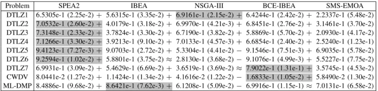
TABLE III
CPF VALUESOBTAINED BYSPEA2, IBEA, NSGA-III, BCE-IBEA,ANDSMS-EMOAON3-OBJECTIVEDTLZ1–DTLZ7, CWDV,AND8-OBJECTIVE
ML-DMP, AVERAGEDOVER30 RUNS. THEBESTRESULT INEACHROW ISHIGHLIGHTED.
Problem SPEA2 IBEA NSGA-III BCE-IBEA SMS-EMOA
DTLZ1 6.5305e-1 (2.25e-2)+ 5.6315e-1 (3.35e-2)+ 6.9161e-1 (2.15e-2)+ 6.4244e-1 (2.42e-2)+ 2.2337e-1 (5.48e-2) DTLZ2 7.0532e-1 (2.60e-2)+ 4.0179e-1 (3.18e-2)+ 6.9970e-1 (4.21e-3)+ 6.8451e-1 (2.76e-2)+ 3.1461e-1 (3.70e-2) DTLZ3 7.3148e-1 (2.33e-2)+ 3.7824e-1 (3.30e-2)+ 6.7190e-1 (3.82e-2)+ 5.8869e-1 (5.70e-2)+ 2.0930e-1 (4.17e-2) DTLZ4 7.1266e-1 (3.30e-2)+ 3.9213e-1 (9.10e-2)+ 7.0133e-1 (4.57e-3)+ 6.6854e-1 (2.40e-2)+ 2.5240e-1 (1.23e-1) DTLZ5 9.4123e-1 (7.27e-3)+ 9.0703e-1 (2.72e-2)+ 5.3304e-1 (4.41e-2)− 9.1546e-1 (7.51e-3)+ 6.9035e-1 (5.78e-2) DTLZ6 9.2594e-1 (1.02e-2)+ 5.8801e-1 (3.75e-2)≈ 2.8130e-1 (3.68e-2)− 9.1076e-1 (4.99e-3)+ 5.5227e-1 (7.75e-2) DTLZ7 6.9931e-1 (3.09e-2)+ 5.4629e-1 (6.69e-2)+ 3.6519e-1 (3.69e-2)≈ 7.9022e-1 (1.31e-1)+ 3.5745e-1 (4.53e-2) CWDV 8.0441e-2 (1.27e-2)+ 1.1424e-1 (1.34e-2)+ 4.1616e-2 (1.22e-2)− 1.6833e-1 (1.05e-2)+ 5.8490e-2 (1.30e-2) ML-DMP 8.4886e-1 (9.68e-2)+ 8.6421e-1 (7.62e-3)+ 6.1208e-1 (5.09e-2)− 6.9916e-1 (1.15e-1)≈ 7.0131e-1 (6.58e-2)
is less uniform than that obtained by BCE-IBEA. NSGA-III and SMS-EMOA obtain the bestCLµ values on DTLZ5 and
DTLZ6, respectively, as they obtained fewer solutions than the other MOEAs on DTLZ5 and DTLZ6. However, it is obvious that the solution sets obtained by SPEA2 and BCE-IBEA have better diversity. Similarly, IBEA obtains the best PD value on DTLZ5 and DTLZ6, which is due to the outliers (i.e., extreme solutions) in the solution sets. NSGA-III obtains the best IGD and ∆p values on DTLZ2 and DTLZ4, since the reference
points have the same distribution as the solution set obtained by NSGA-III. In fact, the solution sets obtained by SPEA2 and BCE-IBEA have better evenness than those obtained by NSGA-III on DTLZ2 and DTLZ4. NSGA-III also obtains the best HV values on DTLZ2 and DTLZ4, which is attributed to the fact that most solutions obtained by it are on the border, which are biased by the HV metric. To summarize, none of the above metrics can accurately reflect the diversity performance of the compared MOEAs on DTLZ1–DTLZ7, CWDV, and ML-DMP.
By contrast, according to Table III, it can be found that the CPF values are consistent with the observations obtained from Fig. 1 in the Supplementary Materials. Specifically, NSGA-III has the best diversity performance on DTLZ1, SPEA2 has the best diversity performance on DTLZ2–DTLZ4, SPEA2 and BCE-IBEA have similar diversity performance on DTLZ5– DTLZ6, BCE-IBEA has the best diversity performance on DTLZ7 and CWDV, and IBEA has the best diversity perfor-mance on ML-DMP. Moreover, the box plots of the above seven metric values are shown in Fig. 2 in the Supplementary Materials. It can be seen that the variance of the CPF values is low, and each MOEA has significantly different CPF values. By contrast, the variance of other metric values are relatively high on some test instances, and all the MOEAs have very similar metric values on some other test instances. Therefore, the effectiveness of the proposed CPF in diversity assessment is confirmed.
On the other hand, it can be observed from Fig. 1 in the Supplementary Materials that the difference between the diversity performance of SPEA2 and BCE-IBEA is negligible on most MOPs. This is mainly due to the fact that most of the test MOPs have simplex-like Pareto fronts, making it easy for MOEAs to obtain a diverse solution set once they converge to the Pareto front. In order to better compare the diversity performance of different MOEAs, a multi-objective test suite containing various complex Pareto fronts is proposed in the
next section.
IV. PROPOSEDMULTI-OBJECTIVETESTSUITE
A. Existing Multi-Objective Test Suites
ZDT is one of the first multi-objective test suites [42], which contains six bi-objective MOPs. The Pareto fronts of ZDT3 and ZDT5 are discontinuous and discrete, respectively, and the Pareto fronts of all the others are continuous curves. In general, many existing MOEAs (e.g., NSGA-II [20] and MOEA/D [43]) are capable of obtaining a set of solutions with good diversity on the Pareto fronts of ZDT problems.
DTLZ and WFG are the two most widely used test suites [30], [44], which are scalable with respect to both decision variables and objectives. DTLZ contains seven unconstrained MOPs and two constrained MOPs, and WFG contains nine unconstrained MOPs. The Pareto fronts of DTLZ5, DTLZ6, DTLZ8, DTLZ9, and WFG3 are mostly degenerate, the Pareto fronts of DTLZ7 and WFG2 are discontinuous, and the Pareto fronts of all the others are simplex-like surfaces. In addition, several variants of DTLZ problems have been proposed for improving the difficulty in diversity preservation [7], [45]. Nevertheless, some state-of-the-art MOEAs (e.g., BCE-IBEA [36] and AR-MOEA [9]) show satisfactory diversity perfor-mance on most DTLZ and WFG problems.
Recently, the MaF test suite was proposed for the CEC 2017/2018 competition on evolutionary many-objective opti-mization [46]. MaF contains 15 scalable MOPs with various Pareto fronts, and introduces difficulty for MOEAs to obtain a set of diverse solutions in high-dimensional space. However, such difficulty is highly alleviated when the number of objec-tives is just two or three.
Apart from the above multi-objective test suites, there also exist a number of test suites in the literature [3], [47], [48]. However, these test suites mainly focus on testing the convergence performance of MOEAs, and most benchmark MOPs in these test suites have simplex-like Pareto fronts. Therefore, in order to better compare the diversity performance of different MOEAs, a multi-objective test suite containing various complex Pareto fronts is proposed in the following.
B. The Proposed Test Suite
In order to make an MOP focus on testing the diversity performance of MOEAs, the following two principles are followed:
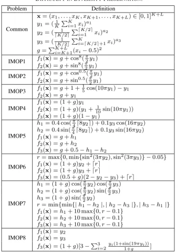
TABLE IV
DEFINITION OF THEPROPOSEDMULTI-OBJECTIVETESTSUITE, WHERE
KANDLAREPARAMETERSCONTROLLING THELENGTH OFDECISION
VARIABLES,ANDa1,a2,ANDa3AREPARAMETERSCONTROLLING THE
DIFFICULTY INDIVERSITYPRESERVATION.
Problem Definition Common x= (x1, . . . , xK, xK+1, . . . , xK+L)∈[0,1]K+L y1= (K1 ∑Ki=1xi)a1 y2= (⌈K/12⌉∑i⌈=1K/2⌉xi)a2 y3= (⌊K/12⌋∑Ki=⌈K/2⌉+1xi)a3 g=∑Ki=+KL+1(xi−0.5)2 IMOP1 f1(x) =g+ cos 8(π 2y1) f2(x) =g+ sin8(π2y1) IMOP2 f1(x) =g+ cos 0.5(π 2y1) f2(x) =g+ sin0.5(π2y1) IMOP3 f1(x) =g+ 1 + 1 5cos(10πy1)−y1 f2(x) =g+y1 IMOP4 f1(x) = (1 +g)y1 f2(x) = (1 +g)(y1+101 sin(10πy1)) f3(x) = (1 +g)(1−y1) IMOP5
h1= 0.4 cos(π4⌈8y2⌉) + 0.1y3cos(16πy2)
h2= 0.4 sin(π4⌈8y2⌉) + 0.1y3sin(16πy2)
f1(x) =g+h1
f2(x) =g+h2
f3(x) =g+ 0.5−h1−h2
IMOP6
r= max{0,min{sin2(3πy2),sin2(3πy3)} −0.05}
f1(x) = (1 +g)y2+⌈r⌉ f2(x) = (1 +g)y3+⌈r⌉ f3(x) = (0.5 +g)(2−y2−y3) +⌈r⌉ IMOP7 h1= (1 +g) cos(π2y2) cos(π2y3) h2= (1 +g) cos(π2y2) sin(π2y3) h3= (1 +g) sin(π2y2) r= min{min{|h1−h2|,|h2−h3|},|h3−h1|} f1(x) =h1+ 10 max{0, r−0.1} f2(x) =h2+ 10 max{0, r−0.1} f3(x) =h3+ 10 max{0, r−0.1} IMOP8 f1(x) =y2 f2(x) =y3 f3(x) = (1 +g)[3−∑3i=2 yi(1+sin(19πyi)) 1+g ]
• The Pareto front should be complex enough, which can pose stiff challenges for MOEAs in diversity preservation. Meanwhile, it should be possible to sample a set of uniformly distributed reference points on the Pareto front for performance assessment.
• It should be easy to obtain solutions on the Pareto front, which enables MOEAs to quickly obtain a set of well-converged solutions and thus spend most computational resources in diversifying these solutions for better diver-sity.
Following the above two principles, we design a multi-objective test suite consisting of three bi-multi-objective MOPs and five three-objective MOPs with irregular Pareto fronts, namely, IMOP1–IMOP8. The definitions of the eight MOPs are given in Table IV, where x denotes a solution and
f1(x), f2(x), . . . denote its objective values. In general, a
solution x = (x1, . . . , xK+L) consists of two parts, where x1, . . . , xK determine the position of the solution on the Pareto
front and xK+1, . . . , xK+L determine the distance from the
solution to the Pareto front. A solution is on the Pareto front only if it satisfies g= 0, i.e., xK+1, . . . , xK+L= 0.5; hence
the Pareto optimal set satisfies Ω ⊆ [0,1]K × {0.5}L. As a result, it is fairly easy to obtain well-converged solutions for the eight proposed MOPs. More importantly, since there is no linkage between the decision variables, it is possible to
diversify well-converged solutions to any part of the Pareto fronts.
Nevertheless, obtaining a set of solutions with a good evenness and spread for these MOPs is still difficult. On one hand, the decision variables determining the positions of solutions on the Pareto fronts are biased by parameters a1,
a2 anda3, which has been recognized as a major factor that
makes the solutions difficult to maintain a proper diversity [49]. Note that the values of a1, a2 and a3 should be larger
than zero, and an extremely small or large value indicates a great difficulty in diversity preservation. On the other hand, the Pareto fronts of all the eight proposed MOPs are highly irregular, which is also a challenge to most existing MOEAs [50].
As shown in Fig. 9, the Pareto fronts of IMOP1 and IMOP2 are one-dimensional convex and concave curves with sharp tails, respectively, where the extreme solutions are difficult to be preserved by MOEAs. The Pareto front of IMOP3 is a one-dimensional discontinuous curve, where MOEAs are likely to miss some parts of the Pareto front. Similarly, the Pareto fronts of IMOP4–IMOP8 are all irregular surfaces in three-dimensional space. To be specific, the Pareto front of IMOP4 is a wavy line, the Pareto front of IMOP5 consists of eight circles, the Pareto front of IMOP6 is separated into several grids, and the Pareto front of IMOP7 is a part of a unit sphere in the first octant. It is worth noting that the Pareto front of IMOP8 contains 100 discontinuous subregions and each subregion contains infinite points, although it looks like a continuous plane. As a consequence, the Pareto front shapes of IMOP1–IMOP8 are considerably different from those in existing test suites, and some of them can represent real-world scenarios. For example, according to the non-dominated solutions obtained on real-world MOPs, some Pareto fronts of real-world MOPs are curves with sharp tails like IMOP1 [51], some Pareto fronts contain several disconnected parts like IMOP5 [31], and some Pareto fronts are degenerated surfaces in three-dimensional space like IMOP4 [52].
It is worth noting that a set of uniformly distributed ref-erence points sampled on the Pareto front are needed for the calculation of many performance metrics (e.g., IGD and∆p).
Generally, it is not an easy task to sample uniformly distributed reference points on irregular Pareto fronts, and so far no much research has been done to address this issue [41], [53]–[55]. In order to better use the proposed test suite in assessing the performance of MOEAs, the mathematical formulations of the Pareto fronts as well as the methods for sampling a set of uniformly distributed reference points on the Pareto fronts are given in Supplementary Materials II.
C. Experimental Results on the Proposed Test Suite
This subsection verifies the effectiveness of the proposed test suite in distinguishing between the diversity performance of MOEAs. To this end, the five MOEAs compared in Sec-tion III are tested on the proposed test suite with the same parameter settings. Besides, the parameters K,L,a1,a2 and
a3 in IMOP1–IMOP8 are set to 5, 5, 0.05, 0.05 and 10,
0 f 1 1 0 1 f2 IMOP1 0 f 1 1 0 1 f2 IMOP2 -0.1 f 1.2 1 0 0.9 f 2 IMOP3 0 0 0 f 3 IMOP4 f 1 f2 1 1 1 -0.2 -0.5 -0.5 f3 IMOP5 f 2 f1 1.2 0.5 0.5 0 0 0 IMOP6 f3 f 1 f 2 1 1 1 0 0 0 f 3 IMOP7 f 1 f 2 1 1 1 -0.9 0 0 IMOP8 f 3 f 1 f 2 3 1 1
Fig. 9. The Pareto fronts of the proposed multi-objective test suite.
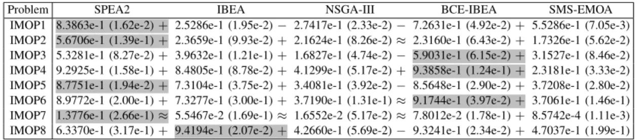
TABLE V
CPF VALUESOBTAINED BYSPEA2, IBEA, NSGA-III, BCE-IBEA,ANDSMS-EMOAONIMOP1–IMOP8, AVERAGEDOVER30 RUNS. THEBEST
RESULT INEACHROW ISHIGHLIGHTED.
Problem SPEA2 IBEA NSGA-III BCE-IBEA SMS-EMOA
IMOP1 8.3863e-1 (1.62e-2)+ 2.5286e-1 (1.95e-2)− 2.7417e-1 (2.33e-2)− 7.2631e-1 (4.92e-2)+ 5.5286e-1 (7.05e-3) IMOP2 5.6706e-1 (1.39e-1)+ 2.3659e-1 (9.93e-2)+ 2.1624e-1 (8.26e-2)≈ 2.3160e-1 (6.43e-2)+ 1.7326e-1 (5.62e-2) IMOP3 5.3281e-1 (8.27e-2)+ 3.9632e-1 (1.21e-1)+ 1.6827e-1 (4.74e-2)− 5.9031e-1 (6.15e-2)+ 3.1527e-1 (8.46e-2) IMOP4 9.2925e-1 (1.58e-1)+ 8.4805e-1 (8.78e-2)+ 4.1299e-1 (5.17e-2)+ 9.3858e-1 (1.24e-1)+ 2.3181e-1 (3.33e-2) IMOP5 8.7751e-1 (1.94e-2)+ 7.3104e-1 (3.75e-2)+ 3.4081e-1 (3.92e-2)− 8.5648e-1 (2.90e-2)+ 3.7208e-1 (2.80e-2) IMOP6 8.9772e-1 (2.00e-1)+ 7.3277e-1 (3.00e-1)+ 3.7190e-1 (1.31e-1)≈ 9.1744e-1 (3.97e-2)+ 3.7061e-1 (1.46e-1) IMOP7 1.3776e-1 (2.66e-1)≈ 5.5467e-2 (1.69e-1)≈ 1.6552e-2 (5.17e-2)≈ 7.8012e-2 (1.78e-1)+ 8.5742e-4 (1.11e-3) IMOP8 6.3370e-1 (3.17e-1)+ 9.4194e-1 (2.07e-2)+ 4.2660e-1 (5.69e-2)− 9.3241e-1 (2.34e-2)+ 4.7037e-1 (1.99e-1)
The non-dominated solution sets obtained by SPEA2, IBEA, NSGA-III, BCE-IBEA, and SMS-EMOA on IMOP1–IMOP8 are presented in Fig. 3 in the Supplementary Materials. From the figure, it can be observed that the five compared MOEAs exhibit significantly different diversity performances on the eight MOPs. To be specific, for IMOP1–IMOP4 whose Pareto fronts are irregular curves in bi- or three-dimensional space, SPEA2 shows the best diversity performance on IMOP1 and IMOP2, while the solution set obtained by BCE-IBEA has the best diversity on IMOP3 and IMOP4. For IMOP5 whose Pareto front contains eight circles, all the compared MOEAs are able to find a set of solutions covering the whole Pareto front, but the solutions obtained by NSGA-III and SMS-EMOA are of poor distribution. For IMOP6 whose Pareto front consists of several grids, SPEA2, IBEA, and BCE-IBEA show better diversity performance than the other MOEAs. IMOP7 is quite challenging to the compared MOEAs, such that none of solution sets obtained by all the MOEAs can cover the whole Pareto front. As for IMOP8, the diversity performance of IBEA and BCE-IBEA is significantly better than that of the other MOEAs.
Table V lists the CPF values of the obtained solution sets, and the box plots of the CPF values are depicted in Fig. 4 in the Supplementary Materials. The reference point set used in the CPF calculation contains roughly 10,000 reference points on the Pareto front of each MOP. According to Table V, SPEA2 has the best diversity performance on IMOP1, IMOP2, IMOP5, and IMOP7, BCE-IBEA has the best diversity per-formance on IMOP3, IMOP4, and IMOP6, and IBEA has
the best diversity performance on IMOP8. Therefore, it can be concluded that SPEA2, IBEA, and BCE-IBEA have better overall diversity performance than the other compared MOEAs on the proposed test suite.
To summarize, we can conclude from the above experi-mental results that the compared MOEAs show significantly different diversity performances on the proposed test suite; however, none of them is able to obtain a solution set with satisfactory diversity on all the eight MOPs. Therefore, it is confirmed that the proposed test suite can distinguish between the diversity performance of MOEAs, and pose challenges for them to obtain a solution set with good diversity.
V. CONCLUSIONS
This paper has proposed a performance metric and a multi-objective test suite for diversity assessment in evolutionary multi-objective optimization. The proposed metric assesses both the evenness and spread of a given solution set by projecting it to a lower-dimensional hypercube and calculating the “volume” of it. The proposed metric has been empirically demonstrated to be superior over existing metrics in diversity assessment. The proposed test suite contains eight MOPs with irregular Pareto fronts, which is verified to be capable of distinguishing between the diversity performance of MOEAs, and posing tough challenges for MOEAs to obtain a set of solutions with satisfactory diversity.
While the proposed metric CPF focuses on assessing the diversity of a given solution set, it is interesting to enhance the
proposed metric CPF to assess both convergence and diversity. On one hand, CPF can be combined with some metrics assess-ing only convergence like GD [16], where the metric value can be defined as a weighted sum of the original CPF value and the GD value of each solution. On the other hand, it is desirable to extend CPF to the assessment of both convergence and diversity by monopolized hypercube. In addition, since the difficulty of diversity preservation increases rapidly with the number of objectives, test problems involving more objectives can be designed to pose challenges for MOEAs to obtain diverse solutions in a high-dimensional space.
ACKNOWLEDGEMENT
This work was supported in part by the National Nat-ural Science Foundation of China under Grant 61672033, 61822301, U1804262, Anhui Provincial Natural Science Foundation for Distinguished Young Scholars under Grant 1808085J06, State Key Laboratory of Synthetical Automation for Process Industries under Grant PAL-N201805, and Shen-zhen Peacock Plan under Grant KQTD2016112514355531. The work of Y. Jin was supported in part by the U.K. EPSRC under Grant EP/M017869/1.
REFERENCES
[1] A. Zhou, B.-Y. Qu, H. Li, S.-Z. Zhao, P. N. Suganthan, and Q. Zhang, “Multiobjective evolutionary algorithms: A survey of the state of the art,”Swarm and Evolutionary Computation, vol. 1, no. 1, pp. 32–49, 2011.
[2] T. Ulrich, “Pareto-set analysis: Biobjective clustering in decision and objective spaces,”Journal of Multi-Criteria Decision Analysis, vol. 20, no. 5-6, pp. 217–234, 2013.
[3] Q. Zhang, A. Zhou, and Y. Jin, “RM-MEDA: A regularity model-based multiobjective estimation of distribution algorithm,”IEEE Transactions on Evolutionary Computation, vol. 12, no. 1, pp. 41–63, 2008. [4] X. Zhang, Y. Tian, R. Cheng, and Y. Jin, “A decision variable
clustering-based evolutionary algorithm for large-scale many-objective optimiza-tion,”IEEE Transactions on Evolutionary Computation, vol. 22, no. 1, pp. 97–112, 2018.
[5] M. Li, S. Yang, and X. Liu, “Shift-based density estimation for Pareto-based algorithms in many-objective optimization,”IEEE Transactions on Evolutionary Computation, vol. 18, no. 3, pp. 348–365, 2014. [6] C. He, Y. Tian, Y. Jin, X. Zhang, and L. Pan, “A radial space division
based evolutionary algorithm for many-objective optimization,”Applied Soft Computing, vol. 61, pp. 603–621, 2017.
[7] K. Deb and H. Jain, “An evolutionary many-objective optimization algorithm using reference-point based non-dominated sorting approach, part I: Solving problems with box constraints,”IEEE Transactions on Evolutionary Computation, vol. 18, no. 4, pp. 577–601, 2014. [8] R. Cheng, Y. Jin, M. Olhofer, and B. Sendhoff, “A reference vector
guided evolutionary algorithm for many-objective optimization,”IEEE Transactions on Evolutionary Computation, vol. 20, no. 5, pp. 773–791, 2016.
[9] Y. Tian, R. Cheng, X. Zhang, F. Cheng, and Y. Jin, “An indicator based multi-objective evolutionary algorithm with reference point adaptation for better versatility,”IEEE Transactions on Evolutionary Computation, vol. 22, no. 4, pp. 609–622, 2018.
[10] Y. Sun, G. G. Yen, and Z. Yi, “IGD indicator-based evolutionary algo-rithm for many-objective optimization problems,”IEEE Transactions on Evolutionary Computation, vol. 23, no. 2, pp. 173–187, 2019. [11] H. Wang, Y. Jin, and X. Yao, “Diversity assessment in many-objective
optimization,”IEEE Transactions on Cybernetics, vol. 47, no. 6, pp. 1510–1522, 2017.
[12] L. K. Hansen and P. Salamon, “Neural network ensembles,” IEEE Transactions on Pattern Analysis & Machine Intelligence, vol. 12, no. 10, pp. 993–1001, 2002.
[13] J. R. Schott, “Fault tolerant design using single and multicriteria genetic algorithm optimization,” Master’s thesis, Department of Aeronautics and Astronautics, Massachusetts Institute of Technology, 1995.
[14] J. Wu and S. Azarm, “Metrics for quality assessment of a multiobjective design optimization solution set,” Journal of Mechanical Design, vol. 123, no. 1, pp. 18–25, 2001.
[15] A. Zhou, Y. Jin, Q. Zhang, B. Sendhoff, and E. Tsang, “Combining model-based and genetics-based offspring generation for multi-objective optimization using a convergence criterion,” inProceedings of the 2006 IEEE Congress on Evolutionary Computation, 2006, pp. 892–899. [16] D. A. V. Veldhuizen and G. B. Lamont, “Multiobjective evolutionary
algorithm research: A history and analysis,” Department of Electrical and Computer Engineering. Graduate School of Engineering, Air Force Inst Technol, Wright Patterson, Tech. Rep. TR-98-03, Tech. Rep., 1998. [17] K. Deb and S. Jain, “Running performance metrics for evolutionary multi-objective optimization,” Indian Institute of Technology, KanGAL Technical Report 2002004, Tech. Rep., 2002.
[18] L. While, P. Hingston, L. Barone, and S. Huband, “A faster algorithm for calculating hypervolume,”IEEE Transactions on Evolutionary Com-putation, vol. 10, no. 1, pp. 29–38, 2006.
[19] M. Li, S. Yang, and X. Liu, “Diversity comparison of Pareto front approximations in many-objective optimization,”IEEE Transactions on Cybernetics, vol. 44, no. 12, pp. 2568–2584, 2014.
[20] K. Deb, A. Pratap, S. Agarwal, and T. Meyarivan, “A fast and elitist multi-objective genetic algorithm: NSGA-II,” IEEE Transactions on Evolutionary Computation, vol. 6, no. 2, pp. 182–197, 2002.
[21] K. Fang and C. Ma,Orthogonal and Uniform Experimental Design. Science and Technology Press, Beijing, 2001.
[22] C. Luo, “Point spatial analyses–fractal dimension and uniform index,”
Science & Technology Review, vol. 10, pp. 51–54, 2004.
[23] A. Solow, S. Polasky, and J. Broadus, “On the measurement of biolog-ical diversity,”Journal of Environmental Economics and Management, vol. 24, no. 1, pp. 60–68, 1993.
[24] C. A. Coello Coello, G. B. Lamont, and D. A. Van Veldhuizen, Evo-lutionary Algorithms for Solving Multi-Objective Problems. Springer, 2007.
[25] O. Sch¨utze, X. Esquivel, A. Lara, and C. A. C. Coello, “Using the averaged hausdorff distance as a performance measure in evolutionary multiobjective optimization,”IEEE Transactions on Evolutionary Com-putation, vol. 16, no. 4, pp. 504–522, 2012.
[26] I. Das and J. E. Dennis, “Normal-boundary intersection: A new method for generating the Pareto surface in nonlinear multicriteria optimization problems,”SIAM Journal on Optimization, vol. 8, no. 3, pp. 631–657, 1998.
[27] K. Li, K. Deb, Q. Zhang, and S. Kwong, “Combining dominance and decomposition in evolutionary many-objective optimization,”IEEE Transactions on Evolutionary Computation, vol. 19, no. 5, pp. 694–716, 2015.
[28] R. Denysiuk, L. Costa, and I. E. Santo, “Clustering-based selection for evolutionary many-objective optimization,” in Proceedings of the International Conference on Parallel Problem Solving from Nature, 2014, pp. 538–547.
[29] J. Cheng, G. Yen, and G. Zhang, “A many-objective evolutionary algorithm with enhanced mating and environmental selections,” IEEE Transactions on Evolutionary Computation, vol. 19, pp. 592–605, 2015. [30] K. Deb, L. Thiele, M. Laumanns, and E. Zitzler, “Scalable test problems for evolutionary multiobjective optimization,” inEvolutionary Multiob-jective Optimization, 2005, pp. 105–145.
[31] X. Liao, Q. Li, X. Yang, W. Zhang, and W. Li, “Multiobjective optimization for crash safety design of vehicle using stepwise regression model,”Struct Multidisc Optim, vol. 35, pp. 561–569, 2007.
[32] M. Li, C. Grosan, S. Yang, X. Liu, and X. Yao, “Multiline distance minimization: A visualized many-objective test problem suite,” IEEE Transactions on Evolutionary Computation, vol. 22, no. 1, pp. 61–78, 2018.
[33] Y. Tian, R. Cheng, X. Zhang, and Y. Jin, “PlatEMO: A MATLAB platform for evolutionary multi-objective optimization,”IEEE Compu-tational Intelligence Magazine, vol. 12, no. 4, pp. 73–87, 2017. [34] E. Zitzler, M. Laumanns, and L. Thiele, “SPEA2: Improving the strength
Pareto evolutionary algorithm for multiobjective optimization,” in Pro-ceedings of the Fifth Conference on Evolutionary Methods for Design, Optimization and Control with Applications to Industrial Problems, 2001, pp. 95–100.
[35] E. Zitzler and S. K¨unzli, “Indicator-based selection in multiobjective search,” inProceedings of the 8th International Conference on Parallel Problem Solving from Nature, 2004, pp. 832–842.
[36] M. Li, S. Yang, and X. Liu, “Pareto or non-Pareto: Bi-criterion evolution in multi-objective optimization,” IEEE Transactions on Evolutionary Computation, vol. 20, no. 5, pp. 645–665, 2016.
[37] N. Beume, B. Naujoks, and M. Emmerich, “SMS-EMOA: Multiobjec-tive selection based on dominated hypervolume,”European Journal of Operational Research, vol. 181, no. 3, pp. 1653–1669, 2007. [38] X. Zhang, Y. Tian, R. Cheng, and Y. Jin, “An efficient approach to
non-dominated sorting for evolutionary multi-objective optimization,”IEEE Transactions on Evolutionary Computation, vol. 19, no. 2, pp. 201–213, 2015.
[39] K. Deb,Multi-Objective Optimization Using Evolutionary Algorithms. New York: Wiley, 2001.
[40] K. Deb and M. Goyal, “A combined genetic adaptive search (GeneAS) for engineering design,”Computer Science and Informatics, vol. 26, no. 4, pp. 30–45, 1996.
[41] Y. Tian, X. Xiang, X. Zhang, R. Cheng, and Y. Jin, “Sampling reference points on the Pareto fronts of benchmark multi-objective optimization problems,” inProceedings of the 2018 IEEE Congress on Evolutionary Computation, 2018, in press.
[42] E. Zitzler, K. Deb, and L. Thiele, “Comparison of multiobjective evolutionary algorithms: Empirical results,”Evolutionary Computation, vol. 8, no. 2, pp. 173–195, 2000.
[43] Q. Zhang and H. Li, “MOEA/D: A multi-objective evolutionary al-gorithm based on decomposition,”IEEE Transactions on Evolutionary Computation, vol. 11, no. 6, pp. 712–731, 2007.
[44] L. B. S. Huband, P. Hingston and L. While, “A review of multiobjective test problems and a scalable test problem toolkit,”IEEE Transactions on Evolutionary Computation, vol. 10, no. 5, pp. 477–506, 2006. [45] H. Jain and K. Deb, “An evolutionary many-objective optimization
algorithm using reference-point based nondominated sorting approach, part II: Handling constraints and extending to an adaptive approach,”
IEEE Transactions on Evolutionary Computation, vol. 18, no. 4, pp. 602–622, 2014.
[46] R. Cheng, M. Li, Y. Tian, X. Zhang, S. Yang, Y. Jin, and X. Yao, “A benchmark test suite for evolutionary many-objective optimization,”
Complex & Intelligent Systems, vol. 3, no. 1, pp. 67–81, 2017. [47] R. Cheng, Y. Jin, M. Olhofer, and B. Sendhoff, “Test problems for
large-scale multiobjective and many-objective optimization,”IEEE Transac-tions on Cybernetics, vol. 47, no. 12, pp. 4108–4121, 2017.
[48] H.-L. Liu, F. Gu, and Q. Zhang, “Decomposition of a multiobjective optimization problem into a number of simple multiobjective subprob-lems,”IEEE Transactions on Evolutionary Computation, vol. 18, no. 3, pp. 450–455, 2014.
[49] K. Deb, “Multi-objective genetic algorithms: Problem difficulties and construction of test problems,”Evolutionary computation, vol. 7, no. 3, pp. 205–230, 1999.
[50] H. Ishibuchi, Y. Setoguchi, H. Masuda, and Y. Nojima, “Performance of decomposition-based many-objective algorithms strongly depends on Pareto front shapes,”IEEE Transactions on Evolutionary Computation, vol. 21, no. 2, pp. 169–190, 2017.
[51] J. Brankea, M. Stein, K. Deb, and H. Schmeck, “Portfolio optimization with an envelope-based multi-objective evolutionary algorithm,” Euro-pean Journal of Operational Research, vol. 199, no. 3, pp. 684–693, 2009.
[52] X. Zhang, F. Duan, L. Zhang, F. Cheng, Y. Jin, and K. Tang, “Pattern rec-ommendation in task-oriented applications: A multi-objective perspec-tive [application notes],”IEEE Computational Intelligence Magazine, vol. 12, no. 3, pp. 43–53, 2017.
[53] G. Rudolph, H. Trautmann, S. Sengupta, and O. Sch¨utze, “Evenly spaced Pareto front approximations for tricriteria problems based on triangulation,” inProceedings of the 7th International Conference on Evolutionary Multi-Criterion Optimization, vol. 7811, 2013, pp. 443– 458.
[54] C. Dominguez-Medina, G. Rudolph, O. Schutze, and H. Trautmann, “Evenly spaced Pareto fronts of quad-objective problems using PSA partitioning technique,” inProceedings of the 2013 IEEE Congress on Evolutionary Computation, 2013, pp. 3190–3197.
[55] H. Trautmann, G. Rudolph, C. Dominguez-Medina, and O. Sch¨utze, “Finding evenly spaced Pareto fronts for three-objective optimization problems,” inEVOLVE - A Bridge between Probability, Set Oriented Numerics, and Evolutionary Computation II. Advances in Intelligent Systems and Computing, vol. 175, 2013, pp. 89–105.