Evolutionary Game Theoretic Multi-Objective Optimization Algorithms and Their Applications

(1)

University of Massachusetts Boston

ScholarWorks at UMass Boston

Graduate Doctoral Dissertations Doctoral Dissertations and Masters Theses

5-31-2017

Evolutionary Game Theoretic Multi-Objective

Optimization Algorithms and Their Applications

Yi Ren Cheng

University of Massachusetts Boston

Follow this and additional works at:https://scholarworks.umb.edu/doctoral_dissertations

Part of theComputer Sciences Commons

Recommended Citation

Ren Cheng, Yi, "Evolutionary Game Theoretic Multi-Objective Optimization Algorithms and Their Applications" (2017).Graduate Doctoral Dissertations. 340.

(2)

EVOLUTIONARY GAME THEORETIC MULTI-OBJECTIVE OPTIMIZATION ALGORITHMS AND THEIR APPLICATIONS

A Dissertation Presented by

YI REN CHENG

Submitted to the Office of Graduate Studies, University of Massachusetts Boston,

in partial fulfillment of the requirements for the degree of

Doctor of Philosophy

May 2017

(3)

(4)

EVOLUTIONARY GAME THEORETIC MULTI-OBJECTIVE OPTIMIZATION ALGORITHMS AND THEIR APPLICATIONS

A Dissertation Presented by

YI REN CHENG

Approved as to style and content by:

Junichi Suzuki, Associate Professor Chairperson of Committee

Dan A. Simovici, Professor Member

Ding Wei, Associate Professor Member

Alfred G. Noel, Professor Member

Dan A. Simovici, Program Director Computer Science Program

Peter Fejer, Chairperson Computer Science Department

(5)

ABSTRACT

EVOLUTIONARY GAME THEORETIC MULTI-OBJECTIVE OPTIMIZATION ALGORITHMS AND THEIR APPLICATIONS

May 2017

Yi Ren Cheng,

B.A., University of Ramon Llull, Spain M.E., University of Ramon Llull, Spain M.S., University of Massachusetts Boston Ph.D., University of Massachusetts Boston

Directed by Associate Professor Junichi Suzuki

Multi-objective optimization problems require more than one objective functions to be optimized simultaneously. They are widely applied in many science fields, including engi-neering, economics and logistics where optimal decisions need to be taken in the presence of trade-offs between two or more conflicting objectives. Most of the real world multi-objective optimization problems are NP-Hard problems. It may be too computationally costly to find an exact solution but sometimes a near optimal solution is sufficient. In these cases Multi-Objective Evolutionary Algorithms (MOEAs) provide good approximate solutions to problems that cannot be solved easily using other techniques. However Evo-lutionary Algorithm is not stable due to its random nature, it may produces very different results every time it runs. This dissertation proposes an Evolutionary Game Theory (EGT) framework based algorithm (EGTMOA) that provides optimality and stability at the same

(6)

to form a novel and promising algorithm to solve multi-objective optimization problems. This dissertation studies three different multi-objective optimization applications, Cloud Virtual Machine Placement, Body Sensor Networks, and Multi-Hub Molecular Commu-nication along with their proposed EGTMOA framework based algorithms. Experiment results show that EGTMOAs outperform many well known multi-objective evolutionary algorithms in stability, performance and runtime.

(7)

ACKNOWLEDGEMENTS

It is a long journey to complete this dissertation. I can not accomplish it without all your helps. Here, I would like to deliver my most sincerely gratitude to the following.

My advisor Prof. Junichi Suzuki, for the continuous support of my Ph.D study and related research, for his patience, motivation, guidance and immense knowledge.

Dr. Dan Simovici, Dr. Wei Ding, and Dr. Alfred Noel for their insightful comments and encouragement. And thank you for being part of my thesis committee.

Computer Science Department faculty, for their tutoring with excellent courses and for providing useful academic resources. Computer Science staff, for their great help in my academic administration and guidance.

My friends Thamer Altuwaiyan, Nada Attar, Dung Phan, Ting Zhang, Quynh Vo, Tong Wang, Kaixun Hua for their accompany, friendship and support through all my academic years in UMASS Boston.

A big thanks to my parents (Jianwei Ren and Xinguang Cheng) and my parents in law (Guanghui Xiao and Hong Wang), for their giving love without any returns and for their constantly support and guidance in my entire life.

My daughter Jana Ren, for well behaved and being a good kid supporting her father during all these time.

In the end I would like to specially thanks my wife Wen Xiao Ren, for being an excellent life partner, a responsible and patient mother, a lovely and brilliant wife. Your love is the fuel that allows me to do the impossible.

(8)

4.5. AGEGT . . . 53

4.6. Cielo-LP . . . 69

5. Body Sensor Network . . . 101

5.1. Introduction . . . 101

5.2. State of the art . . . 102

5.3. Problem Formulation . . . 103 5.4. BitC . . . 110 5.5. Experiment . . . 115 5.6. Conclusion . . . 121 6. Molecular Communication . . . 133 6.1. Introduction . . . 133 6.2. Problem Formulation . . . 135 6.3. EMMCO . . . 140 6.4. Experiment . . . 142 6.5. Conclusion . . . 144 7. Conclusion . . . 149 8. Future Directions . . . 150 8.1. Noise Handling . . . 150 8.2. Speeding Up . . . 150 8.3. Fairness . . . 151

8.4. Cloud simulator extension . . . 151

(10)

LIST OF TABLES

Table Page

1. Message Arrival Rate and Message Processing Time . . . 81

2. Cielo Simulation Settings . . . 81

3. P-states in Intel Core2 Quad Q6700 . . . 82

4. Cielo Execution Time Comparison . . . 82

5. Performance of Cielo, FFA and BFA . . . 83

8. Parameter Settings for AGEGT . . . 87

9. Constraint Combinations . . . 87

10. Impacts of Distribution Index Values on Hypervolume (HV) Per-formance in AGEGT . . . 88

11. Convergence Speed of AGEGT, EGT-GLS, EGT and NSGA-II . . 88

12. Comparison of AGEGT and NSGA-II with Distance Metrics . . . 88

13. Comparison of AGEGT, NSGA-II, FFA and BFA in Objective Values 89 14. Stability of Objective Values in AGEGT and NSGA-II . . . 90

(11)

18. Constraint Combinations . . . 93 19. Impacts of Distribution Index Values on Hypervolume (HV)

Per-formance in Cielo-LP . . . 93

20. Impacts of LP Rates on the Execution Time Performance . . . 93

21. Performance Improvement of Cielo-LPs against Cielo-BASE . . . 98

22. Comparison of Objective Values and Execution Time betweenCielo−

LP_{W S}and Linear Programming . . . 98

23. Comparison of Convergence Speed between Cielo-BASE andCielo−

LP_{W S} . . . 98

24. Comparison of Objective Values amongCielo−LP_{W S}, NSGA-II,

FFA and BFA . . . 99

25. Stability of Objective Values inCielo−LP_{W S}and NSGA-II . . . . 100

26. Body Sensor Networks Simulation Settings . . . 126 27. Energy Harvesting Configurations . . . 127 28. Constraint Combinations . . . 127 29. Impacts of Distribution Index Values on Hypervolume (HV) . . . . 128

30. Comparison of BitC’s Variants in Hypervolume . . . 128

31. Comparison of BitC-HV and NSGA-II . . . 128

32. Stability of Objective Values in BitC-HV and NSGA-II . . . 129

33. Objective Values of BitC-HV under Different Constraint Combi-nations . . . 129 34. Comparison of BitC-HV and NSGA-II in BSN Lifetime and Data

(12)

35. Notation table . . . 132 36. Molecular Communication Simulation Settings . . . 147 37. Performance comparison of EMMCO and Random Search . . . 148

(13)

LIST OF FIGURES

Figure Page

1. A multi-objective optimization problem: buying a used car . . . 1

2. Example of a Pareto curve and Pareto front of two objective functions 3 3. Geometrical representation of the weight-sum approach in the non-convex Pareto curve case . . . 4

4. Geometrical representation of the ε-constraints approach in the non-convex Pareto curve case . . . 5

5. An example of multi-objective optimization problem with two con-flicting objectives . . . 11

6. Search spaces in multi-objective optimization problems . . . 12

7. Three Pareto solutions for data center problem . . . 13

8. A concise work flow of Evolutionary Algorithm . . . 14

9. EA is highly unstable, it may produces very different results in each run. . . 15

10. Prisoner’s Dilemma . . . 17

11. Evolution process in Evolutionary Game Theory . . . 22

12. Dividing the entire whole multi-objective problem intoMsub prob-lems. . . 24

13. Evolution workflow of a population in Baseline EGTMOA algo-rithm. . . 25

(14)

16. An example of polynomial mutation with 6 decision variables. . . . 29

17. Three-Tiered Application Architecture . . . 39

18. Example of Cielo Deployment Strategies . . . 46

19. Cielo Pareto Dominance . . . 52

20. Cielo Hypervolume . . . 53

21. Cielo Hypervolume & Pareto Dominance . . . 54

22. Cielo Hypervolume Comparison . . . 55

23. AGEGT Example Deployment Strategies . . . 57

24. Objective Values of AGEGT under Two Constraint Combinations . 64 25. Objective Values of EGT-GLS under Two Constraint Combinations 65 26. Objective Values of EGT under Two Constraint Combinations . . . 66

27. Comparison of AGEGT, EGT-GLS and EGT in Hypervolume (HV) 67 28. Trajectory of AGEGT’s Solution through Generations . . . 68

29. Cielo-LP Example Deployment Strategies . . . 71

30. Cielo-BASE’s Objective Values with and without Constraints (C_M andC_∞ . . . 94

31. Cielo−LP_{W S}’s Objective Values w/ & w/o Constraints (C_M and C_∞). LP rate: 0.5% . . . 95

32. Cielo−LPW S’s Objective Values w/ & w/o Constraints (CM and C_∞). LP rate: 5% . . . 96

33. Cielo−LP_{W S}’s Objective Values w/ & w/o Constraints (CM and C_∞). LP rate: 10% . . . 97

(15)

34. Trajectory of Cielo-LP’s Solution through Generations . . . 100

35. A Push-Pull Hybrid Communication in BitC . . . 105

36. Virtual sensor communication diagram . . . 106

37. Local Search Comparison . . . 118

38. Three-dimensional Objective Spaces . . . 119

39. 20 BSNs and 100 BSNs performance comparison . . . 131

40. Diffusive communication . . . 136

41. Directional communication . . . 136

42. Stop-and-Wait Automatic Repeat Request communication protocol 137 43. Illustration of a multi-hub intra-body molecular communication . . 139

44. Objective Values of EMMCO with distance between transmitter and receiver 30µm . . . 144

(16)

CHAPTER 1

INTRODUCTION

Many real world problems are often require to satisfy multiple criterion at the same time. Those problems are called multi-objective optimization problems where more than one objective are presented and need to be optimized simultaneously. We could find those kind of problems everywhere in the world, and anytime around our ordinary life. For instance buying a used car we may consider minimizing the cost and mileage while maximizing the MPH (mileage per hour), or designing an aircraft that need to satisfy hundreds of criteria (speed, capacity, energy consumption, acquisition cost, assembly hours, etc...).

(17)

Multi-objective optimization problems often deal with multiple conflicting objectives and may subject to many constraints. In the case of buying a used car Fig. 1, we could have several constraints such as our budget, acceptable mileage, manufacture years, car brand and model, so on. Due to its computational complexity and the huge solution space presented, it has always been a challenge solving multi-objective optimization problems.

In fact, most of real-life multi-objective optimization problems are often of exponential size, a straightforward reduction from the knapsack problem shows that they are NP-hard to compute. Thus, it is computationally too costly to find an exact optimal solution if one exists. And most of the time in real applications it is quite hard for the decision maker to have all the information to correctly and completely formulate them. Therefore, in such sit-uations finding a near optimal solution is a practical approach that fits into multi-objective optimization problems.

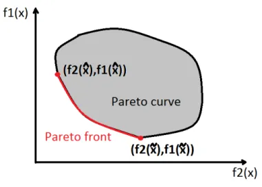
The set of all feasible solutions is called Pareto curve or surface Fig. 2 which represents the solution space of the multi-objective optimization problem. Due to conflicting objec-tives and constraints multi-objective optimization problems lead to not a single optimal solution, but a set of non-dominated solutions which is called Pareto front Fig. 2. More details about Pareto optimal solutions will be given in section 2.1.

Numerous researches have been studied with many different methods proposed to solve multi objective optimization problems. In the next section we are going to review a little what historically have done and what the current state of the art is in question.

1.1 Related works

Many techniques to solve multi-objective optimization problems were proposed in the past. In the following we will start revising some of the most relevant techniques described in

(18)

Figure 2: Example of a Pareto curve and Pareto front of two objective functions

• The Weighted-sum method

The basic idea is to combine multiple objectives into one single-objective scalar function in order to solve a multi-objective problem. This approach is also know as weighted-sum or scalarization method. The goal is to minimize a positively weighted sum of the objectives.

min n

∑

i=1 γi·fi(x) n

∑

i=1 γi=1 γi>0,i=1, ...,n x∈S

After combining multiple objectives into one single objective we have a new opti-mization problem with an unique objective function. Two main drawbacks are pre-sented in this approach. The first one is the possibly huge computation time involved

(19)

by considering different weight values. And when the Pareto curve is non-convex Fig. 3 there is a set of points that cannot be reached for any combination of the weight vector.

Figure 3: Geometrical representation of the weight-sum approach in the non-convex Pareto curve case

• ε-constraints Method

The decision maker chooses one objective out ofnto be minimized, and the

remain-ing objectives are constrained to be less than or equal to given target values.

min fj(x)

f_i(x)≤εi,∀i∈ {1, ...,n} \ {j} x∈S

One advantage of theε-constraints method is that it is able to achieve efficient points in a non-convex Pareto curve. In Fig. 4, when f2(x) =ε2,f1(x)is an efficient point

(20)

Figure 4: Geometrical representation of the ε-constraints approach in the non-convex Pareto curve case

The drawback of this method is that the decision maker has to choose appropriate

upper bounds εi values for the constraints. Moreover, the method is not efficient if

the number of objective functions is greater than two. • Multi-level Programming

Multi-level programming aims to find one optimal point in the entire Pareto surface.

Multi-level programming optimizes the nobjectives in a predefined order. It firstly

minimizes the first objective function, and then it searches for minimizing the sec-ond most important objective, and so on until all the objective function have been optimized.

It works if the order among objectives is meaningful and user is not interested in the continuous trade off among the functions. The main drawback is that the less impor-tant objective functions tend to have no influence on the overall optimal solution. • Goal Programming

(21)

Goal Programming attempts to find specific meta values of these objectives. In fact, it does not solve directly a multiple objectives optimization problem, it tries to find a solution that accomplishes a specific goal. An example is shown below.

f1(x)≥v1

f₂(x) =v₂ f₃(x)≤v₃

x∈S

• Evolutionary Algorithm

Most recent studies focus on evolutionary algorithms (EA) which shown to be a promising method solving multi-objective optimization problems with conflicting objectives by approximating the Pareto solution set. EA is inspired by biological evolution, it uses biologic mechanisms such as reproduction, mutation, crossover, and selection. More details will be given later in section 2.2.

The main advantage is that EAs are metaheuristic algorithms, they do not make any assumption about the underlying fitness landscape. Therefore EA often perform well approximating solutions to all types of problems in many diverse fields as engineer-ing, biology, economics, marketengineer-ing, social sciences, so on.

Some of the most well known EAs are

– Genetic Algorithm: Probably this is the most popular type of EA. GAs are

commonly used to generate high quality solution set by relying on biological inspired operators such as mutation, crossover and selection. Non-dominated Sorting Genetic Algorithm - II known as NSGA-II and Strength Pareto

(22)

Evolu-tionary Algorithm 2 also known as SPEA-2 are well known variants of GA that have become as GA standard approaches.

– Differential Evolution: DE optimizes a problem by maintaining a population of

candidate solutions and to create new candidate solutions by combining existing ones using a differential equation. And then keeping the solution with the best fitness value on the optimization problem at hand.

The main drawback of EA is that it relies heavily on stochastic mechanism, due to its random nature EA is highly unstable in general. Unstable here means under the same problem setting EA could give a very different performance result for each run.

1.2 Contributions

The main goal of this dissertation is to propose a novel algorithm Evolutionary Game Theo-retic Multi-Objective Algorithms (EGTMOA) Chapter 3 that aims to solve multi-objective optimization problems considering stability, optimality and running time. EGTMOA is an Evolutionary Game Theory framework based Evolutionary Algorithm. It combines the sta-bility property from EGT and the optimality notion from EA together to form a new type of metaheuristic algorithm that guarantees to deliver a stable and high quality solution in a reasonable running time. Main contributions are listed as follow.

1. Evolutionary Game Theoretic Multi-Objective Algorithms (EGTMOA): a new meta-heuristic algorithm framework EGTMOA is proposed to solve multi-objective opti-mization problems in a stable, optimal and fast manner.

2. Cloud Virtual Machine Deployment: Formulation of a new multi-objective optimiza-tion problem with four objectives and four constraints that is designed to describe the resource allocation problem in a Cloud Data Center.

(23)

3. Cielo, AGEGT, and Cielo-LP: Description of three EGTMOA framework based al-gorithms that are aimed to solve the formulated Cloud Virtual Machine Deployment multi-objective optimization problem. Their evaluation are performed and studied through different experiments.

4. Body Sensor Network: Creating a new multi-objective optimization problem that attempting to formulate a constrained data transmitting scheduling problem for in-body sensor networks environment

5. BitC: Another EGTMOA framework based algorithm that is designed to solve the Body Sensor Network problem. Evaluation of EGTMOA is performed and studied through different experiments.

6. Molecular Communication: It simulates an in-body Multi-Hub Molecular Commu-nication environment, and formulates a new non-constrained two objective optimiza-tion problem to improve its communicaoptimiza-tion performance and efficiency

7. EMMCO: A variant of EGTMOA algorithm that is proposed to solve the Multi-Hub Molecular Communication problem. Evaluation of EMMCO is performed and studied through different experiments.

1.3 Workflow

The rest of dissertation is organized as follow: Chapter 2 provides an overview of related concepts that lays foundation for this dissertation. Chapter 3 gives in detail all the compo-nents of the proposed approach EGTMOA. In Chapter 4, 5 and 6 I describe three different multi-objective optimization applications, Cloud Virtual Machine Deployment, Body Sen-sor Network, and Multi-Hub Molecular Communication with their respective proposed

(24)

the main contributions of this dissertation, and Chapter 8 discusses potential future research directions originated from this thesis.

(25)

CHAPTER 2

BACKGROUND

2.1 Multi-Objective Optimization

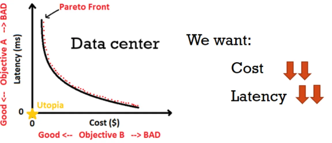
Many classical optimization problem consists of optimizing a single objective, for instance finding the shortest path from an origin to a destination in a network is one of the most classical optimization problems in transportation and logistic. However most of real-life problems in nature have several and possibly conflicting objectives to be satisfied simul-taneously. Fig. 5 shows an example of a multi-objective optimization problem with two conflicting objectives, where we try to find an optimal solution that minimizing the cost of a data center while reducing its data transmission latency. Here in this example the cost could be money that is spent on Internet connection, data center power consumption, hard-ware equipments, so on. And it is not hard to conclude that more money we spent better equipments and connectivity we have, thus as consequence faster the data transmission is and less latency we could have. Since our objective is to minimize the cost and latency, it is clear that these two objectives are conflicting with each other. The utopia point represents the best ideal solution to the formulated problem that usually is not possible to be reached. In this case it is(0,0)which means it costs 0$ to have a latency of 0ms, and of course this is not possible.

(26)

Figure 5: An example of multi-objective optimization problem with two conflicting objec-tives

In mathematical terms, a multi-objective optimization problem can be formulated as follow.

min(f₁(x),f₂(x), ...,f_k(x)) s.t. x∈_X

Wherex∈_Rn_{is a vector of}_n_{decision variables which represent the values to be chosen}

in the optimization problem. _X⊆_Rn_{denotes the feasible set that is implicitly determined}

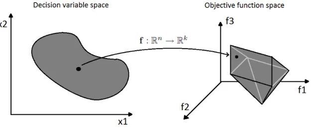
by a set of equality and inequality constraints. f :_Rn →_Rk _{is a vector of} _k _objective

functions that mapndecision variables tokobjective values Fig. 6. In multi-objective

op-timization, the sets_Rnand_Rkare known as decision variable space and objective function

space respectively.

The ultimate goal in a multi-objective optimization problem is to find an optimal so-lution that satisfy simultaneously all the objectives, however multi-objective optimization problems often do not exist a single solution that optimizes each objective at the same time

(27)

Figure 6: Search spaces in multi-objective optimization problems

because of conflicting objectives. In this case, there exists a number of Pareto optimal solutions.

2.1.1 Pareto Optimal Solutions

The set of all feasible solutions is called Pareto curve or surface Fig. 2 which represents the solution space of the multi-objective optimization problem. A solution is called Pareto optimal, if none of the objective functions can be improved in value without degrading some of the other objective values. And the set of Pareto optimal solutions forms Pareto front, where all solution are non-dominated with each other.

Considering the data center example in Fig. 5 let’s give three solutions with respective objective values {S1= (30ms,420K$),S2= (15ms,380K$),S3= (10ms,400K$)}Fig. 7. It is clear thatS2 outperformsS1 in both objectives latency and cost. HoweverS2is better thanS₃in cost objective value, but worst in latency. ThereforeS₂andS₃are non-dominated with each other, and they both belong to the Pareto front set.

(28)

Figure 7: Three Pareto solutions for data center problem

2.2 Multi-Objective Evolutionary Algorithms

Many real world multi-objective optimization problem are NP-Hard Problems. It is not feasible to use brute force search for solving those problems due to the huge amount of computation involved. It is too computationally costly to find an exact solution but some-times a near optimal solution is sufficient. In these cases MOEAs provide good approxi-mate solutions to problems that cannot be solved easily using other techniques. EA uses biological evolution inspired mechanisms, such as mutation, crossover, and selection. Fig.

8 shows a concise work flow of Evolutionary Algorithm whereX_nis the vector of decision

variables andY_mis the vector of objectives.

MOEAs are stochastic search and optimization methods that lead a population of can-didate solutions toward the Pareto front through evolutionary mechanism and biological operators. Algorithm 2.2.1 shows steps that a traditional EA follows. Candidate solutions also called individuals in EA term are set of different decision variable vectors that are randomly generated initially (Line 2). EAs uses mutation and crossover operators to

(29)

gen-Figure 8: A concise work flow of Evolutionary Algorithm

erate new offspring solutions from the original population (Line 5). Later these solutions are evaluated by fitness functions which are objective functions defined by the optimization problem (Line 6). And based on the quality or fitness values of solutions EAs uses selection operator to chose the best non-dominated solution set to form a new population (Line 7). This whole process iterates many times or generations until it satisfies the termination con-dition.

MOEAs presents many advantages over traditional multi-objective approaches:

• MOEAs attempts to search the whole Pareto front instead of one single Pareto opti-mal solution in each run.

• MOEAs do not require any domain knowledge about the problem to be solved • MOEAs do not make any assumption about the Pareto curve.

MOEAs do not guarantee to find the true Pareto optimal set, but instead aim to generate a good approximation of such set in a reasonable computational time. The main drawback

(30)

Algorithm 2.2.1:Evolutionary Algorithm Pseudo-code

1: t←0;

2: InitPopulation[P(t)]; (Initializes the population)

3: EvalPopulation[P(t)]; (Evaluates the population)

4: whilenot terminationdo

5: P0(t)←Variation[P(t)](Creation of new individuals)

6: EvalPopulation[P0(t)]; (Evaluates the new individuals)

7: P(t+1)←ApplyGeneticOperators[P0(t)]; (Creation of next generation population)

8: t←t+1;

9: end while

here means, despite of initial condition, the algorithm always could reach to the same or similar solution in the end if ones exists. Under the same problem setting, EA may produces very different results every time Fig. 9. Therefore researchers usually take the average result across different runs to evaluate MOEAs performance, which is not reliable since we could never guarantee its performance every time we run it.

(31)

In order to overcome EAs stability issue, we will borrow the stability property from Evolutionary Game Theory which is described in the next section 2.3.

2.3 Game Theory

Game Theory is a study of strategic decision making of conflict and cooperation among intelligent rational decision makers. It is an interactive decision theory which means in a game, given a set of strategies, each player strives to find a strategy that optimizes its own payoff depending on the others strategy decisions. Game theory seeks such strategies for all players as a solution, called Nash equilibrium (NE), where no players can gain extra payoff by unilaterally changing his strategy.

2.3.1 Nash equilibrium

Nash equilibrium is a solution concept in which no player has anything to gain by changing only their own strategy. In a two player game, it is a strategy pair. LetE(S,T)represent

the payoff for playing strategy S against strategy T. The strategy pair (S,S) is a Nash

equilibrium in a two player game if and only if this is true for both players and for all

T 6=S.

E(S,S)≥E(T,S)

To illustrate the concept of Game Theory and Nash Equilibrium, let’s take a look at the classical well known Prisoner’s Dilemma Fig. 10. In this game there are two players, prisoner A and B. Each of them has two strategy to chose confess or remain silent. The point is depending on each prisoner’s choice they would have different sentences.

(32)

2. If A confess but B remains silent, then A will be set free and B will serve 20 years in prison (and vice versa).

3. If A and B both confess, then each of them serves 5 years in prison

Figure 10: Prisoner’s Dilemma

In the case 1, prisoner A or B would go free if they switch their own strategy while another one remains the same. In the case 2, prisoner A or B would serve 15 less years if they switch their own strategy while another one remains the same. Therefore by definition both case 1 and 2 are not Nash equilibrium solution. The only Nash equilibrium in this game is the case 3, where none of prisoners could gain extra payoff by switching their own strategy.

(33)

2.4 Evolutionary Game Theory

Evolutionary Game Theory is an application of Game Theory to biological contexts for analyzing population dynamics and stability in biological systems. In EGT, each player maintains a population which is formed by a set of strategies and games are played repeat-edly by strategies randomly drawn from the population. In general, EGT considers two major components, Evolutionarily stable strategies (ESS), and Replicator Dynamics (RD).

2.4.1 Evolutionary Stable Strategy

An Evolutionary Stable Strategy (ESS) is anequilibrium refinementof theNash equilibrium. It is a Nash equilibrium that is evolutionarilystable: once it appearsin a population,natural selectionalone is sufficient to prevent alternative (mutant) strategies from invading success-fully. ESS specifies two conditions for a strategySto be an ESS, for allT 6=S, either

E(S,S)>E(T,S)or

E(S,S) =E(T,S)andE(S,T)>E(T,T)

The first condition is called a strict Nash equilibrium. The second condition means that although strategyT is neutral with respect to the payoff against strategyS, the population

of players who continue to play strategyShas an advantage when playing againstT.

Suppose all players in the initial population are programmed to play a certain (incum-bent) strategyk. Then, let a small population share of players,x∈(0,1), mutate and play

a different (mutant) strategy `. When a player is drawn for a game, the probabilities that

its opponent playskand` are 1−xandx, respectively. Thus, the expected payoffs for the player to play kand ` are denoted asU(k,x`+ (1−x)k)andU(`,x`+ (1−x)k), respec-tively.

(34)

Definition 1 A strategy k is said to be evolutionarily stable if, for every strategy`6=k, a certainx¯∈(0,1)exists, such that the inequality

U(k, x`+ (1−x)k)>U(`, x`+ (1−x)k) (2.1)

holds for all x∈(0,x¯).

If the payoff function is linear, Equation 2.1 derives:

(1−x)U(k,k) +xU(k, `)>(1−x)U(`,k) +xU(`, `) (2.2)

Ifxis close to zero, Equation 2.2 derives either

U(k,k)>U(`,k)or U(k,k) =U(`,k)and U(k, `)>U(`, `) (2.3)

This indicates that a player associated with the strategykgains a higher payoff than the ones associated with the other strategies. Therefore, no players can benefit by changing

their strategies fromkto the others. This means that an ESS is a solution on a Nash

equi-librium. An ESS is a strategy that cannot be invaded by any alternative (mutant) strategies that have lower population shares.

2.4.2 Replicator Dynamics

The replicator dynamics is a model of evolution that describes how population shares as-sociated with different strategies grows over time [TJ78]. Replicator dynamics assumes infinite population size, continuous infinite time, and complete mixing. Complete mixing means pairwise strategies are completely random chosen from the population.

(35)

Letλk(t)≥0 be the number of players who play the strategyk∈K, whereK is the set

of available strategies. The total population of players is given byλ(t) =∑_k|K₌|₁λ_k(t). Let

x_k(t) =λk(t)/λ(t)be the population share of players who playkat timet. The population

state is defined by X(t) = [x₁(t),· · ·,x_k(t),· · ·,x_K(t)]. Given X, the expected payoff of

playing k is denoted byU(k,X). The population’s average payoff, which is same as the

payoff of a player drawn randomly from the population, is denoted byU(X,X) =∑_k|K₌|₁xk· U(k,X).

In the replicator dynamics, the dynamics of the population share x_k is described as

follows. ˙x_k is the time derivative ofx_k.

˙

xk=xk·[U(k,X)−U(X,X)] (2.4)

This equation states that players increase (or decrease) their population shares when their payoffs are higher (or lower) than the population’s average payoff.

Theorem 2.4.1 If a strategy k is strictly dominated, then x_k(t)t→∞→0.

A strategy is said to be strictly dominant if its payoff is strictly higher than any oppo-nents. As its population share grows, it dominates the population over time. Conversely, a strategy is said to be strictly dominated if its payoff is lower than that of a strictly dominant strategy. Thus, strictly dominated strategies disappear in the population over time.

There is a close connection between Nash equilibria and the steady states in the repli-cator dynamics, in which the population shares do not change over time. Since no players change their strategies on Nash equilibria, every Nash equilibrium is a steady state in the replicator dynamics. As described in Section 2.4.2, an ESS is a solution on a Nash

(36)

equi-librium. Thus, an ESS is a solution at a steady state in the replicator dynamics. In other words, an ESS is the strictly dominant strategy in the population on a steady state.

In a conventional game, the objective of a player is to choose a strategy that maximizes its payoff. In contrast, evolutionary games are played repeatedly by all players until a steady point where each player finds their strictly dominant strategy. The strictly dominant strategy in the population is an ESS which is a solution on a Nash Equilibrium that is evolutionarily stable. The Evolutionary game model is illustrated in Fig. 11 and described as follow.

1. The evolution model deals with a Population (G) at generation n. Competition hap-pens among strategies within the population and it is represented by the Game. 2. N/2 Games are performed in each generation. Each Game tests the strategies in

pairwise under the rules of the game. These rules produce different objective payoffs. 3. Based on the payoff the winner replaces the loser in each game.

4. This overall process then produces a new Population (G+1). And the new population then takes the place of the previous one and the cycle begins again (and never stops). 5. It is aniterative process, over time only one strictly dominant strategy will stands in the population, which cannot be invaded by any new mutant strategies. And it is by definition an Evolutionary Stable Strategy (ESS).

(37)

(38)

CHAPTER 3

EVOLUTIONARY GAME THEORETIC MULTI-OBJECTIVE ALGORITHMS (EGTMOA)

Evolutionary Game Theoretic Multi-Objective Algorithms is an Evolutionary Multi-Objective Algorithm designed to follow Evolutionary Game Theory scheme with the goal to seek for a global optimal evolutionarily stable solution. EGTMOA combines the stability property from Evolutionary Game Theory and optimality notion from Evolutionary Algorithms to-gether to form a new metaheuristic multi-objective algorithm that seeks for a set of strict dominant strategies as a global optimal and stable solution through evolution mechanism in a reasonable running time. It has follow properties.

• Optimality: Seeking for a set of strict dominant strategies as a global optimal solu-tion.

• Stability: Providing a stable solution by minimizing oscillations in decision mak-ings.

• Metaheuristic: Just like MOEAs, EGTMOA does not make any assumption about the solution space, and it does not require any domain knowledge about the problem to be solved.

EGTMOA does not guarantee to find a true optimal solution, but instead it provides a high quality stable approximation solution to multi-objective problems at the end.

(39)

3.1 Baseline Algorithm

EGTMOA is an evolutionary algorithm in which the payoff of a strategy is evaluated based on their interactions with other strategies. EGTMOA divides the entire multi-objective

problem intoM sub problems Fig. 12. Each sub problem is handled by an agent or player

that maintains a population of N strategies. And each player seeks a strictly dominant

strategy that maximize its payoff interacting with other players through generations.

Figure 12: Dividing the entire whole multi-objective problem intoM sub problems.

A baseline EGTMOA algorithm is described in Algorithm 3.1.1 and the evolution of a population is illustrated in Fig. 13. EGTMOA has following main steps.

1. Initially random generateNstrategies (decision variables) for each population (Line 2). 2. Random shuffle the order of populations to compute (Line 6).

3. For each population perform N/2 pairwise game evaluation (Line 6-16). A game is carried out based on the superior-inferior relationship between given two strategies and their feasibility (performGame() in Algorithm 3.1.2).

4. Winner duplicates itself, loser is deleted from the population (Line 10,14,15). 5. The duplicated winner has a probability to be mutated (Line 11-13).

(40)

7. Take the feasible strategy with the greatest population share as dominant strategyd_i

(Line 18-22).

8. Return the dominant strategyd_i of each population as a global solution for the

for-mulated Multi-Objective Optimization Problem (Line 26).

Figure 13: Evolution workflow of a population in Baseline EGTMOA algorithm.

3.2 Quality Indicators

From each population we randomly choseN/2 pairwise strategies to play the game

Algo-rithm 3.1.2. In each game a winner and a loser will be determined based on their solution quality. Thus, a game is performed by comparing the fitness values of the chosen pair strategies. These fitness values are computed through objective functions that are defined by multi-objective problems formulation. Since we are dealing with two or more objectives we need a mechanism that helps us to determine the winner and loser in a multi-objective

(41)

point of view. And this mechanism is handled by quality indicator, for the baseline EGT-MOA algorithm we use the Pareto Dominance (PD) notion as our primary quality indicator [SD95]..

3.2.1 Pareto Dominance

Pareto Dominance guarantees the optimality of one strategy over another. It is often called strict dominance quality indicator, because a strategy must have equal or better fitness value in all the objectives in order to become the winner. A strategys₁is said to dominate another strategys₂if both of the following conditions hold:

• s₁’s objective values are superior than, or equal to,s₂’s in all objectives. • s₁’s objective values are superior thans₂’s in at least one objectives.

The dominating strategy wins a game over the dominated one. If two strategies are non-dominated with each other, the winner is randomly selected. To illustrate better the concept of Pareto Dominance, let’s take a look at Fig. 14. Considering a two objective

minimization problem we try to find the best solution among s1,s2 and s3 using Pareto

Dominance notion. From the Fig. 14 we can easily conclude thats2 performs better than

s3 in one objective and worse in another one. Therefores2 ands3 are non-dominated with

each other. And it is clear that s1 performs better in all two objectives than other two

solutions. So we say s1 dominates both s2 ands3. Thus, s1 is the winner after playing

game againsts2 ands3.

3.2.2 Hypervolume

(42)

Figure 14: Quality comparison with two objectives using Pareto Dominance.

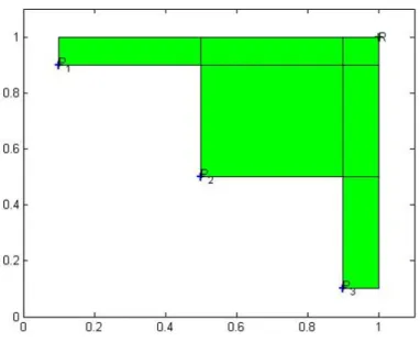
In this case we employ a Hypervolume metric [ZT98] based quality indicator. It measures the volume that a given strategy (s) dominates in the objective space:

HV(s) =Λ

_[

{x0|sx0x_r} (3.1)

Λdenotes the Lebesgue measure.xris the reference point placed in the objective space.

i.e. in Fig. 15 we have three solution points in the objective spaceP1,P2andP3. Rrepresents the reference point, it usually takes the maximum value that each objective function could reach. Now we compute each solution’s Hypervolume value as the rectangle area that is formed by each of the solution point with the reference point. A higher Hypervolume value

means that a solution is more optimal. Thus, P₂is the winner after playing game against

P₂andP₃. It should be noted that before we compute the Hypervolume value, we have to

(43)

Figure 15: Quality comparison with two objectives using Hypervolume.

3.3 Constraints handling

Multi-objective optimization problems often present many constraints which make the problem more realistic, but harder to be solved. Those constraints are defined by a set of equality and inequality functions. EGTMOAs take constraints into account every time a game is performed Algorithm 3.1.2.

If a feasible strategy and an infeasible strategy participate in a game, the feasible one always wins the game. If both strategies are feasible, they are compared using a quality indicator.

If both strategies are infeasible in a game, then they are compared based on their con-straint violation. Concon-straint violation is computed as the difference between the concon-straint value and its cap limit value. An infeasible strategys₁wins a game over another infeasible strategys₂if both of the following conditions hold:

(44)

• s₁’s constraint violation is lower than, or equal to,s₂’s in all constraints. • s₁’s constraint violation is lower thans₂’s in at least one constraints.

3.4 Mutation

After each game the winner duplicates itself and loser is deleted from the population. Due to this dominance notion EGTMOA some time may converges very fast into a local optimal point. In order to prevent the mentioned problem, we need to keep a certain diversity in the population that helps us to move toward a global optimal solution. In this case mutation does the job, it helps us to jump out from a local optimal point. Mutation is a biological operator that is applied with a certain probability to the winner of each game shown in Algorithm 3.1.1 (Line 11-13). Te baseline EGTMOA algorithm uses Polynomial Mutation which is described in the next Section 3.4.1.

3.4.1 Polynomial Mutation

Figure 16: An example of polynomial mutation with 6 decision variables.

In polynomial mutation each decision variable has a probability of 1/v to be mutated,

(45)

within the same range as the original decision variable value. i.e. in Fig. 16v=6, so each decision variable mutates with a probability of 1/6.

3.5 Termination

EGTMOA performs iterative evolution process through generations seeking for the set of strictly dominant strategy as a global optimal solution. In theory the evolution process assumes infinite population size, and continuous infinite time. However in practice this is not feasible, we have to stop the algorithm in some point. Therefore we need to define a termination criteria that tells us when we should stop running our EGTMOA and to get the final solution result. EGTMOA provides two different approaches for defining the termination condition.

• Static termination: Chose a fixed maximum number of generations G based on experiments and empirical results.

• Dynamic termination: EGTMOA ends if the dominant strategy does not improve

more than X% of performance within Y number of generations. Or the dominant

strategy has a population share greater thanZ%. It should be noted that the value of

X,Y andZcome from experiments and empirical results.

Thanks to EGTMOA’s stability property, its convergence curve, speed and performance

are stable as well across different runs which makes the choice of proper X,Y,Z and G

values more reliable. In the next Section 3.6 we are going to see a stability analysis of the proposed algorithm EGTMOA.

(46)

3.6 Stability Analysis

This section analyzes EGTMOA’s stability (i.e., reachability to at least one of Nash equi-libria) by proving the state of each population converges to an evolutionarily stable equil-librium. The proof consists of three steps: (1) designing a set of differential equations that describe the dynamics of the population state (or strategy distribution), (2) proving an strat-egy selection process has equilibria and (3) proving the the equilibria are asymptotically stable (or evolutionarily stable) . The proof uses the following terms and variables.

• Sdenotes the set of available strategies. S∗denotes a set of strategies that appear in the population.

• X(t) ={x1(t),x2(t),· · ·,x|S∗_|(t)}denotes a population state at time t where x_s(t) is the population share of a strategys∈S. ∑s∈S∗(xs) =1.

• F_s is the fitness of a strategys. It is a relative value determined in a game against an opponent based on the dominance relationship between them. The winner of a game earns a higher fitness than the loser.

• ps_k=x_k·φ(Fs−Fk)denotes the probability that a strategysis replicated by winning

a game against another strategyk. φ(Fs−Fk)is the probability that the fitness ofsis

higher than that ofk.

The dynamics of the population share ofsis described as follows.

˙ x_s=

∑

k∈S∗_,_k₆₌_s {xspsk−xkpks}=xs

∑

k∈S∗_,_k₆₌_s x_k{φ(Fs−Fk)−φ(Fk−Fs)} (3.2)

Note that ifsis strictly dominated,x_s(t)t→∞→0.

(47)

Proof It is true that different strategies have different fitness values. In other words, only one strategy has the highest fitness among others. Given Theorem 2.4.1, assuming that F₁ >F₂ >· · ·>F_|_S∗_|, the population state converges to an equilibrium: X(t)_t_→_∞=

{x1(t),x2(t),· · ·,x|S∗|(t)}t→∞={1,0,· · ·,0}.

Theorem 3.6.2 The equilibrium found in Theorem 3.6.1 is asymptotically stable.

Proof At the equilibriumX={1,0,· · ·,0}, a set of differential equations can be downsized by substitutingx1=1−x2− · · · −x|S∗_| ˙ z_s=z_s[c_s₁(1−z_s) + |s∗|

∑

k=2,k6=s z_k·c_sk], s,k=2, ...,|S∗| (3.3)

wherec_sk≡φ(Fs−Fk)−φ(Fk−Fs))andZ(t) ={z2(t),z3(t),· · ·,z|S∗_|(t)}denotes the cor-responding downsized population state. Given Theorem 2.4.1,Z_t_→_∞=Z_eq={0,0,· · ·,0}

of (|S∗| −1)-dimension.

If all Eigenvalues of Jaccobian matrix ofZ(t)has negative real parts,Z_eqis asymptoti-cally stable. The Jaccobian matrixJ’s elements are

(48)

J=         c₂₁ 0 · · · 0 0 c₃₁ · · · 0 .. . ... . .. ... 0 0 · · · c_|_S∗_|₁         (3.5)

(49)

Algorithm 3.1.1:Evolutionary Game Theoretic Multi-Objective Algorithm

1: g= 0

2: Randomly generate the initialNpopulations:P={P₁,P2, ...,PN}

3: whilenot terminationdo

4: foreach populationPirandomly selected fromPdo

5: P_i0← /0

6: for j=1 to|Pi|/2do

7: s1←randomlySelect(Pi)

8: s2←randomlySelect(Pi)

9: winner←performGame(s₁,s₂)

10: replica←replicate(winner)

11: ifrandom()≤Pmthen

12: replica←mutate(winner)

13: end if 14: Pi\ {s1,s2} 15: P_i0∪ {winner,replica} 16: end for 17: Pi←Pi0 18: di←argmaxs∈_Pixs 19: whilediis infeasibledo 20: Pi\ {di} 21: di←argmaxs∈_Pixs 22: end while 23: end for 24: g=g+1 25: end while 26: returnd={d1,d2, ...,dN}

(50)

Algorithm 3.1.2:Game between Strategies - performGame()

Require: s₁ands₂: Strategies to play a game

Ensure: Winner of the game

1: ifs1ands2are feasiblethen

2: ifs₁s₂then 3: return s1 4: end if 5: ifs2s1then 6: return s2 7: end if 8: return randomlySelect({s1,s2}) 9: end if

10: ifs1is feasible ands2is infeasiblethen

11: return s1

12: end if

13: ifs2is feasible ands1is infeasiblethen

14: return s2

15: end if

16: ifs1ands2are infeasiblethen

17: return argmins∈{s1,s2}c

v s

(51)

CHAPTER 4

VIRTUAL MACHINE DEPLOYMENT ON CLOUD DATA CENTER

4.1 Introduction

It is a challenging issue for cloud operators to place applications so that the applications can satisfy given constraints in performance (e.g. response time) while maintaining their re-source utilization (CPU and network bandwidth utilization) and power consumption. The operators are required to dynamically place applications by adjusting their locations and resource allocation according to various operational conditions such as workload and re-source availability. In order to address this challenge, this Chapter investigates three dif-ferent application placement schedulers, Cielo, AGEGT, and Cielo-LP which exhibit the following properties:

• Self-optimization: allows applications to autonomously seek their optimal place-ment configurations (i.e., locations and resource allocation) according to operational conditions (e.g., workload and resource availability), as adaptation decisions, under given optimization objectives and constraints.

• Self-stabilization: allows applications to autonomously seek stable adaptation de-cisions by minimizing oscillations (or non-deterministic inconsistencies) in decision making.

(52)

Cielo, AGEGT, and Cielo-LP are EGTMOA framework based algorithms that approach the self-optimization and self-stabilization properties with Evolutionary Algorithm (EA) and Evolutionary Game Theory (EGT), respectively. In general, EGTMOAs are robust problem-independent search methods that seek optimal solutions (adaptation decisions) with reasonable computational costs by maintaining a small ratio of search coverage to the entire search space [Eib02, Deb01]. EGTMOAs employ EGT as a means to mathematically formulate adaptive decision making and theoretically guarantee that each decision making process converges to an evolutionarily (or asymptotically) stable equilibrium where a spe-cific (stable) adaptation decision is deterministically made under a particular set of opera-tional conditions. EGTMOAs allow applications to seek the solutions to optimally adapt their locations and resource allocation and operate at equilibria by making evolutionarily stable decisions for application placement.

4.2 State of the art

Numerous research efforts have been made to study heuristic algorithms for application placement problems in clouds (e.g., [LQL13, MLL12, GP13, CSV12, LWY09, KBK13, CJH10, WKL10]). Most of them assume a single-tier application architecture and consid-ers a single optimization objective. For example, in [LWY09, KBK13, CJH10, WKL10], only power consumption is considered as the objective. In contrast, I assume a multi-tier application architecture (i.e., three tiers in an application) and considers multiple objec-tives. It is designed to seek a trade-off solution among conflicting objecobjec-tives.

Game theoretic algorithms have been used for a few aspects of cloud computing; for example, application placement [KA09b, WVZ09, DDL07], task allocation [SZL08] and data replication [KA09a]. In [KA09b, WVZ09, DDL07], greedy algorithms seek equilibria

(53)

in application placement problems. This means they do not attain the stability property to reach equilibria as EGTMOAs do.

Several genetic algorithms (e.g., [WSY12, TEC08]) and other stochastic optimization algorithms (e.g., [GGQ13, CWJ13]) have been studied to solve application placement prob-lems in clouds. They seek the optimal placement solutions; however, they do not consider stability. In contrast, EGTMOAs aid applications to seek evolutionarily stable solutions and stay at equilibria.

This study is novel in that EGTMOAs integrate optimization and stabilization processes to seek optimal and stable solutions. Optimization and stabilization have been studied largely in isolation, but few attempts have been made so far to integrate and facilitate them simultaneously, except in a very limited number of work (e.g., [KL03]).

Evolutionary algorithms and other stochastic search algorithms often focus on opti-mization and fail to seek stable solutions [MF04, Kun99, MW96]. As a result, they can inconsistently yield different sets of solutions in different runs/trials with the same prob-lem settings, especially when a given probprob-lem’s search space is large [TD08, YKK08, LZW08, LP07]. Conversely, EGTMOAs are often dedicated to seek stable solutions (i.e., equilibria), which are not necessarily optimal [Wei96, Now06, NRT07].

4.3 Problem Statement

This section formulates an application placement problem to place N applications onM

hosts available in a cloud data center. Each application is designed with a set of server software, following a three-tier application architecture [UPS05, SH06] (Fig. 17).

Using a certain hypervisor such as Xen [BDF03], each server is assumed to run on a virtual machine (VM) atop a host. A host can operate multiple VMs. They share resources

(54)

available on their local host. Each host is assumed to be equipped with a multi-core CPU that supports DVFS in each core.

Each message is sequentially processed from a Web server to a database server through an application server. A reply message is generated by the database server and forwarded in the reverse order toward a user. (Fig. 17). It is assumed that different applications utilize different sets of servers. (Servers are not shared by different applications.) And each host runs multi cores processor to allocate different applications.

Figure 17: Three-Tiered Application Architecture

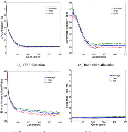
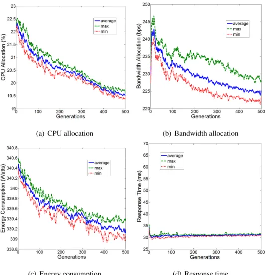
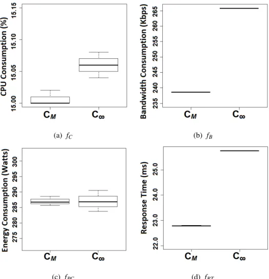
The goal of this problem is to find evolutionarily stable strategies that deployN applica-tions (i.e.,N×3 VMs) onMhosts so that the applications adapt their locations and resource allocation to given workload and resource availability with respect to the four objectives described below. Every objective is computed on an application by application basis and is to be minimized.

• CPU allocation(f_C): A certain CPU time share (in percentage) is allocated to each VM. (The CPU share of 100% means that a CPU core is fully allocated to a VM.) It represents the upper limit for the VM’s CPU utilization. This objective is computed as the sum of CPU shares allocated to three VMs of an application.

f_C= 3

∑

t=1

c_t (4.1)

(55)

• Bandwidth allocation(f_B): A certain amount of bandwidth (in bits/second) is allo-cated to each VM. It represents the upper limit for the VM’s bandwidth consumption. This objective is computed as the sum of bandwidth allocated to three VMs of an ap-plication. f_B= 3

∑

t=1 b_t (4.2)

b_tdenotes the amount of bandwidth allocated to thet-th tier server in an application. • Response time (f_RT): This objective indicates the time required for a message to

travel from a web server to a database server:

fRT =Tp+Tw+Tc (4.3)

Tp denotes the total time for an application to process an incoming message from

a user at three servers. Tw is the waiting time for a message to be processed at

servers. Tc denotes the total communication delay to transmit a message between

servers. Tp, Tw andTc are estimated with the M/M/M queuing model, in which

message arrivals follow a Poisson process and a server’s message processing time is exponentially distributed.

Tpis computed as follows whereT_tpdenotes the time required for thet-th tier server to process a message. Tp= 3

∑

t=1 T_tp (4.4) Twis computed as follows.

(56)

Tw = 1 λ 3

∑

t=1 ρ0 aO_t O! ρt (1−ρt)2 (4.5) wherea_t=λt T_tp c_t·q_t/q_max, ρt= a_t O, ρ0= O−1

∑

n=0 ρ_tn n! + ρ_tO O! 1 1−ρt/O !−1

λ denotes the message arrival rate for an application (i.e., the number of messages

the application receives from users in the unit time). Note thatλ = 1₃∑3_t=1λt where λt is the message arrival rate for the t-th tier server in the application. Currently,

λ =λ1=λ2=λ3. ρt denotes the utilization of a CPU core that thet-th tier server

resides on. q_max is is the maximum CPU frequency. q_t is the frequency of a CPU

core that the t-th tier server resides on. O is the total number of cores that a CPU

contains. Tcis computed as follows. Tc= 2

∑

t=1 T_tc_→_t₊₁≈ 3

∑

t0₌₂ B·λt+1 bt (4.6)

Bis the size of a message (in bits). T_tc_→_t₊₁denotes the communication delay to trans-mit a message from thet-th to(t+1)-th server. bt denotes the bandwidth allocated

to thet-th tier server (bits/second).

• Power Consumption (f_PC): This objective indicates the total power consumption (in Watts) by the CPU cores that operate three VMs in an application.

f_PC= 3

∑

t=1 Pqt idle+ (P qt max−P qt idle)·ct· q_t qmax (4.7)

(57)

Pqt

idleandP

qt

max denote the power consumption of a CPU core that thet-th tier server

resides on when its CPU utilization is 0% and 100% at the frequency ofq_t,

respec-tively.

Four constraints are considered.

• CPU core capacity constraint (C_C): The upper limit of the total share allocation on each CPU core. c_i,o ≤CC for all O cores on all M hosts whereci,o is the total

share allocation on theo-th core of thei-th host. The violation of this constraint is computed as: g_C= M

∑

i=1 O

∑

o=1 I_iC_,_o·(ci,o−CC) (4.8) I_iC_,_o=1 ifo_i>C_C. Otherwise,IC_i_,_o=0.

• Bandwidth capacity constraint (CB): The upper limit of bandwidth consumption

allocated to each host. b_i≤C_B for allM hosts whereb_i is the total amount of band-width allocated to thei-th host. The violation of this constraint is computed as:

gB= M

∑

i=1 I_iB·(bi−CB) (4.9) I_iB=1 ifb_i>C_B. Otherwise,I_iB=0.

• Response time constraint (C_RT): The upper limit of response time for each appli-cation. f_RTi ≤CRT for all applications where f_RTi is the response time of the i-th

application. The violation of this constraint is computed as:

g_RT = N

∑

i=1

(58)

• Power consumption constraint(C_PC): The upper limit of power consumption for

each application. f_PCi ≤C_PC for all N applications where f_PCi is the power

con-sumption of thei-th application. The violation of power consumption constraint is

computed as: g_PC= N

∑

i=1 I_iPC·(f_PCi −CPC) (4.11) I_iPC=1 if f_PCi >C_PC. Otherwise,I_iPC=0.

In this Chapter three different variants of EGTMOA based framework are studied, Cielo, AGEGT, and Cielo-LP. Each of them occupies a Section in this Chapter, and it is organized starting with a brief introduction, following by the algorithm description and it ends with experiment results and conclusions.

4.4 Cielo

This section studies a EGTMOA framework for application placement in clouds that sup-port a power capping mechanism (e.g., Intel’s Runtime Average Power Limit–RAPL) for CPUs. Given the notion of power capping, power can be treated as a schedulable resource in addition to traditional resources such as CPU time share and bandwidth share. The pro-posed algorithm is called Cielo (Sky in Spanish), aids cloud operators to schedule resources (e.g., power, CPU and bandwidth) to applications and place applications onto particular CPU cores in an adaptive and stable manner according to the operational conditions in a cloud, such as workload and resource availability. This study evaluates Cielo through a theoretical analysis and simulations. It is theoretically guaranteed that Cielo allows each application to perform an evolutionarily stable deployment strategy, which is an equilib-rium solution under given operational conditions. Simulation results demonstrate that Cielo

(59)

allows applications to successfully leverage the notion of power capping to balance their response time performance, resource utilization and power consumption.

4.4.1 Introduction

Dynamic Voltage and Frequency Scaling (DVFS) is a major method of choice for inves-tigating the trade-off between power consumption and performance in cloud applications. Power capping is an emerging alternative to DVFS [RAS]. Instead of managing the CPU’s frequency directly, the user simply specifies a time window and a power consumption bound. The CPU guarantees that its average power consumption will not exceed the speci-fied could over each window. Both the window size and bound can be modispeci-fied at runtime. This mechanism treats power as a schedulable resource and allows cloud operators to con-trol the exact amount of power that each CPU consumes.

Given the current availability of power capping mechanisms from major CPU manu-facturers, such as Intel’s Runtime Average Power Limit (RAPL), Cielo focuses on an ap-plication placement problem for cloud operators to schedule resources (e.g., power, CPU and bandwidth) to applications and place applications onto particular CPU cores according to the operational conditions in a cloud, such as workload and resource availability.

Cielo is a variant of EGTMOA framework for adaptive and stable application place-ment in clouds that support a power capping mechanism for CPUs. This section describes its design and evaluates its optimality and stability. In Cielo, each application maintains a set (or a population) of deployment strategies, each of which indicates the location of and resource allocation for that application. Cielo theoretically guarantees that, through a series of evolutionary games between deployment strategies, the population state (i.e., the distribution of strategies) converges to an evolutionarily stable equilibrium, which is al-ways converged to regardless of the initial state. (A dominant strategy in the evolutionarily

(60)

stable population state is called anevolutionarily stable strategy.) In this state, no other strategies except an evolutionarily stable strategy can dominate the population. Given this theoretical property, Cielo aids each application to operate at equilibria by using an evolu-tionarily stable strategy for application deployment in a deterministic (i.e., stable) manner. Simulation results verify this theoretical analysis. Applications seek equilibria to per-form evolutionarily stable deployment strategies and adapt their locations and resource allocations to given operational conditions. Cielo allows applications to successfully lever-age the notion of power capping and balance their response time performance, resource utilization and power consumption. In comparison to existing heuristics, Cielo outper-forms two well-known heuristics algorithm first-fit and best-fit algorithms (FFA and BFA), which have been widely used for adaptive cloud application deployment [LQL13, MLL12, GP13, CSV12].

4.4.2 Algorithm

Cielo maintainsN populations,{P1,P2, ...,PN}, forNapplications and performs games

among strategies in each population. A strategysis defined to indicate the locations of and resource allocation for three VMs in an application:

s(ai) =

[

t∈1,2,3

(hi,t,ci,t,ui,t,bi,t,pi,t), 1<i<N (4.12)

aidenotes thei-th application. hi,tis the ID of a host that operatesai’st-th tier VM.ci,t

is the ID of the core inside the hosth_i,t. ui,t andbi,t are the CPU and bandwidth allocation

(61)

Figure 18: Example of Cielo Deployment Strategies

tier VM. This power cap is translated later to CPU p-state based on the table 3. Each core operates at the highest p-state required by its allocated VMs.

Fig. 18 shows two example strategies for two applications (a1anda2) (N=2 andM= 2). a₁’s strategy (s(a₁)) places the first-tier VM on host 1 core 3(h_1,1=1,c_1,1=3), which

caps power to 90 Watts p1,1=90and consumes 30% CPU share and 80 Kbps bandwidth for

the VM (c_1,1=30 andb_1,1=80). The second-tier VM is placed on host 1 core 3(h_1,2=1,

c1,2=3), which caps power to 100 Watts (p1,2=100) and consumes 30% CPU share and

85 Kbps bandwidth for the VM (c1,2=30 andb1,2=85). The third-tier VM is placed on

host 2 core 3 (h_1,3=2, c_1,3=3), which caps power to 83 Watts p_1,3=83 and consumes

45% CPU share and 120 Kbps bandwidth for the VM (c1,3=45 and b1,3=120). Given

s(a₁), a₁’s objective values for CPU allocation and bandwidth allocation are 105% (30 + 30 + 45) and 285 kbps (80 + 85 + 120).

Algorithm 4.4.1 shows how Cielo seeks an evolutionarily stable strategy for each appli-cation through evolutionary games. In the 0-th generation, strategies are randomly

(62)

gener-ated for each population (Line 2). In each generation (g), a series of games are carried out on every population (Lines 4 to 24). A single game randomly chooses a pair of strategies (s₁ands₂) and distinguishes them to the winner and the loser with respect to the objectives described in Section 4.3 (Lines 7 to 9). The loser disappears in the population. The winner

is replicated to increase its population share and mutated with a certain rate Pm (Lines 10

to 15). Mutation randomly chooses one of three VMs in the winner and alters itsh_i_,_t, c_i_,_t

andbi,t values at random (Line 12).

Once all strategies have played games in the population, Cielo identifies a feasible strategy whose population share (xs) is the highest and determines it as a dominant strategy

(d_i) (Lines 18 to 22). A strategy is said to be feasible if it never violate the CPU and

bandwidth capacity constraints (cv=0 in Eq. 4.8 and bv=0 in Eq. 4.9). It is said to be infeasible ifcv>0 orbv>0. Cielo deploys three VMs for an application in question based on the dominant strategy.

A game is carried out based on the superior-inferior relationship between given two strategies and their feasibility (performGame() in Algorithm 4.4.1). If a feasible strategy and an infeasible strategy participate in a game, the feasible one always wins over its op-ponent. If both strategies are feasible, they are compared with one of the following three schemes to select the winner.

• Pareto dominance (PD): This scheme is based on the notion of dominance

citesrini-vas95multiobjective, in which a strategy s₁ is said to dominate another strategy s₂

(denoted bys1s2) if both of the following conditions hold:

– s₁’s objective values are superior than, or equal to,s₂’s in all objectives. – s₁’s objective values are superior thans₂’s in at least one objectives.

(63)

The dominating strategy wins a game over the dominated one. If two strategies are non-dominated with each other, the winner is randomly selected.

• Hypervolume (HV): This scheme is based on the hypervolume metric [ZT98]. It measures the volume that a given strategy (s) dominates in the objective space:

HV(s) =Λ

_[

{x0|sx0xr}

(4.13)

Λ denotes the Lebesgue measure. xr is the reference point placed in the objective

space. A higher hypervolume means that a strategy is more optimal. Given two strategies, the one with a higher hypervolume value wins a game. If both have the same hypervolume value, the winner is randomly selected.

• Hybrid of Pareto comparison and hypervolume (PD-HV): This scheme is a com-bination of the above two schemes. First, it performs the Pareto dominance (PD) comparison for given two strategies. If they are non-dominated, the hypervolume (HV) comparison is used to select the winner. If they still tie with the hypervolume metric, the winner is randomly selected.

If both strategies are infeasible i