Multi-output structured learning

(1)

(2)

MULTI-OUTPUT STRUCTURED LEARNING

BY

ABNER GUZMAN RIVERA

DISSERTATION

Submitted in partial fulfillment of the requirements

for the degree of Doctor of Philosophy in Computer Science

in the Graduate College of the

University of Illinois at Urbana-Champaign, 2014

Urbana, Illinois

Doctoral Committee:

Professor Rob A. Rutenbar, Chair, Director of Research

Professor David Forsyth

Professor Dan Roth

Assistant Professor Dhruv Batra, Virginia Tech

(3)

Abstract

Real-world applications of Machine Learning (ML) require modeling and reasoning about complex, heterogeneous and high-dimensional data. Probabilistic Inference and Structured-Output Prediction (SOP) are frameworks within ML, which enable systems to learn and reason about complex output spaces by exploiting conditional independence assumptions. SOP systems are capable of coping with exponentially large numbers of possibilities,e.g., all segmen-tations of an image (i.e., labelings of every pixel with a semantic category); all English translations of a Chinese sentence; or all 3D configurations of a fixed-length sequence of (a priori unknown) amino acids. Indeed, SOP has led to state-of-the-art results in applications from various fields [Bakir et al., 2007].

Despite their success and generality, the application of SOP systems to real-world tasks is most severely limited by intractability issues. In brief, intractability is a consequence of high-order interactions in real-world phenomena. For this reason, researchers adopt performance-limiting simplifying assumptions (e.g., of conditional independence) within their models and forgo optimality guarantees in their inference algorithms. Learning SOP models from data is also intractable in general and thus, further approximations are introduced in the learning task. Additionally,labeled training data, is expensive and most often limited and biased. As a consequence of all of these difficulties, the SOP systems used in practice are plagued with limitations and inaccuracies.

Further complicating the above is the fact thatuncertaintyis inherent to real-world applications for SOP,e.g., the data input to SOP systems is noisy, incomplete or otherwise ambiguous – in some cases, the input-output mapping is in effect one-to-many. As a result, the distributions over outputs we are interested to model are in general multi-modal. In this work, we propose to increase the expressivity and performance of SOP models by specifying and training models to producefixed-size tuples of structured-outputs. We achieve this by constructing “portfolios” of structured prediction models that make independent predictions at test-time but that are trained jointly to produce sets ofrelevant and diversehypotheses.

In some sense, the motivation fordecompositionin this thesis is akin to the spirit of mixture models or ensemble approaches. However, in this work we dispense with component weights and delay commitment to single predictions. In doing so, we advocate for pipelined approaches where multiple hypotheses are fed forward for refinement,

(4)

aggre-gation, simulation, etc. or as inputs to increasingly complex predictive tasks. In these settings, it is often practical and advantageous for certain stages to be informed by higher order features (e.g., inter-hypothesis features), additional information available at test-time (e.g., generative procedure, temporal or textual context) or a user/expert in the loop. We show that our methods lead to predictions of higher accuracy compared to current methods and that we are able to leverage multiple predictions to outperform the state-of-the-art in end-to-end applications.

(5)

(6)

Acknowledgments

I gladly take this opportunity to thank every person I encountered during my PhD. Simply, I wouldn’t be the person I am without you and I am grateful to and for each one of you.

Above all, I thank my God, Jesus, for the gift of life and for unrelenting grace and patience. I thank Jesus for His ongoing redeeming work; for being the model of love and humility; and for the hope offered to everyone.

While I couldn’t make individual mentions of everyone I’ve referred to above, I would like to acknowledge some of the people that were directly involved with the research in this thesis:

I’m grateful to my PhD adviser, Rob Rutenbar, for believing I could get the work done when it wasn’t at all clear this was the case; for giving me all freedom to pursue my personal research interests; and for providing funding to make this work happen.

I’m grateful to my collaborators Dhruv Batra and Pushmeet Kohli for the opportunity to associate with them and for the many things they taught me. Clearly, I could not have completed this work without them.

I thank Rob Rutenbar, David Forsyth, Dan Roth, Dhruv Batra and Pushmeet Kohli for serving in my doctoral committee.

I thank Julie Gustafson and Karen Stahl for assisting me many times with administrative and other random matters. I thank my parents, Abelardo and Magdalena, for unconditional and unfaltering love and support. I thank my brother, Abelardo, for his support and for taking care of the family while I’ve been away.

I thank my many roommates and hosts for their hospitality and for keeping living arrangements interesting. Thanks to Abulgasem Shommakhi, Corinne Tellier, Larry Jackson, Rafael Pi˜neiro, Dorothy Brownfield Carlson, James More-land, Andres Velarde, Devin Ruthstrom, and Adam and Alecia Hollinger.

I also thank Daniel Bauer, Jaesik Choi, Jungwook Choi, Glenn Ko and Shang-nien Tsai for their friendship and different forms of assistance through the past few years.

(7)

List of Tables

6.1 DivMCuts with caching on f-b segmentation. . . 75 6.2 DivMCuts with caching on protein side-chain prediction. . . 76

(10)

List of Figures

1.1 Example Structured Prediction tasks. . . 3

1.2 Multi-Output Structured Prediction for the foreground-background segmentation task in Fig. 1.1a. . . 5

1.3 Increased expressivity from learning a “portolio” of predictors (blue) compared to a single predictor (red). . . 6

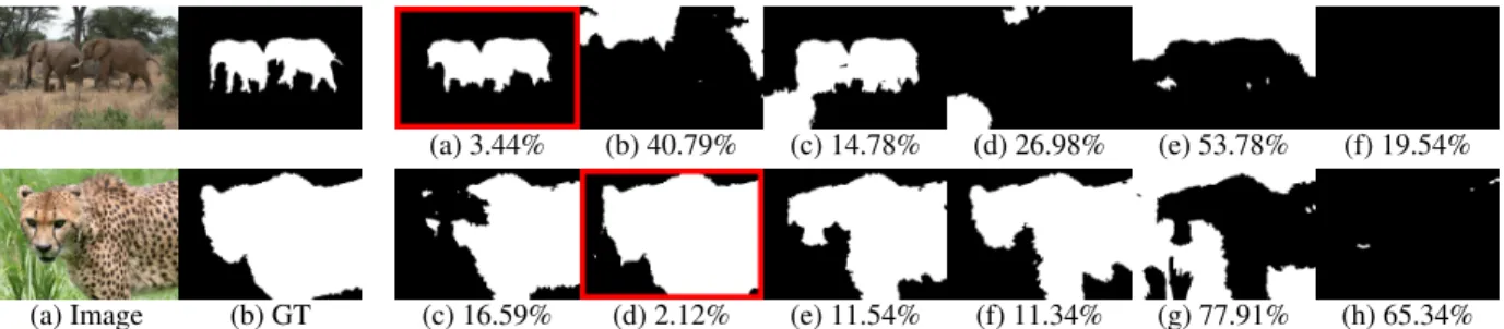
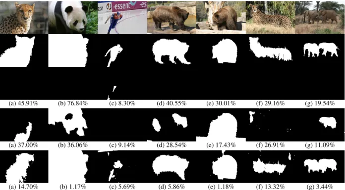
3.1 Each row shows: (a) input image (b) ground-truth segmentation and (c-h) the set of predictions produced by MCL (M=6). Red border indicates the most accurate segmentation (i.e., lowest error). We can see that the predictors produce different plausible foreground hypotheses,e.g., predictor (g) thinks foliage-like things are foreground. . 30

3.2 In each column: first row shows input images; second shows ground-truth; third shows segmentation produced by the single SSVM baseline; and the last two rows show the best MCL predictions (M=6) at the end of the first and last coordinate descent iteration. . . 31

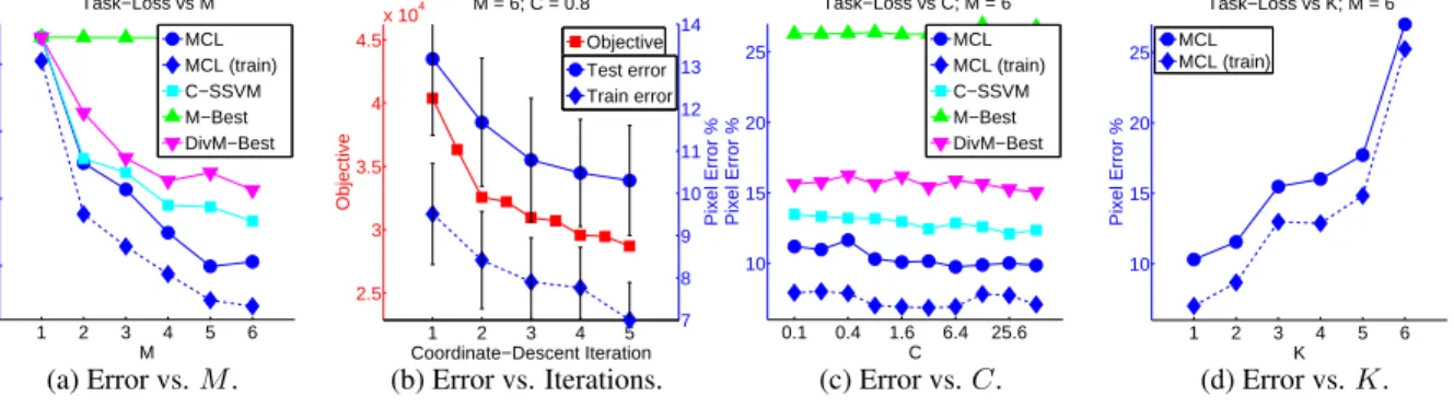
3.3 Experiments on foreground-background segmentation. . . 32

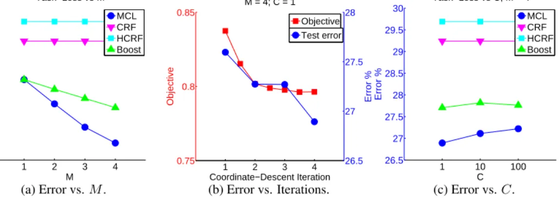
3.4 Experiments on protein side-chain prediction. . . 33

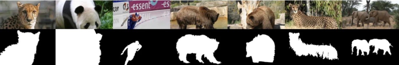
4.1 First row: input images. Second row: corresponding ground-truth segmentations. . . 43

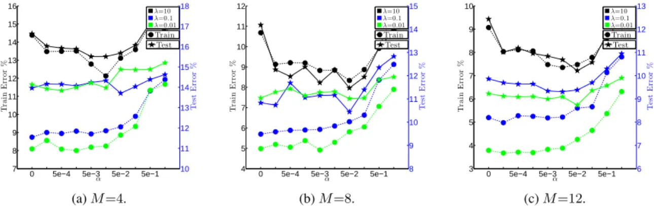
4.2 ForM_{∈ {}4,8,12_}, experiments on coarsened segmentation showing trends as regularization param-eterλ; and diversity-parameterαare varied. We show averages over 5 random folds (1 fold used for training and the remaining for testing). Circles correspond to train-error (left axis) and stars to test-error (right axis). We note that for allλand allM the proposed approach leads to improved test-performance. At high regularization the approach leads to improved train and test test-performance. As expected, at low regularizationαmodulates fit to train and often leads to improved test performance. . 44

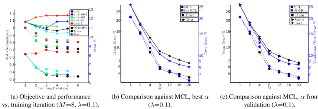
4.3 Experiments on coarsened segmentation (averages over 5 random folds). (a) Behavior of coordinate descent (M=8,λ=0.1). Thediversified-riskis plotted on the left-axis (squares); and train, test errors are plotted on the right-axis (circles, stars). Note howαmodulates fit to train nicely and that certain values ofαlead to test-time improvements. (b) Comparison against MCL baseline asM increases,α tuned on test. (c) Comparison against MCL baseline asM increases,αtuned on held-out data. We observe that the proposed approach leads to performance improvements over a range ofM. . . 45

4.4 Experiments on segmentation (averages over 5 random folds). Circles correspond to train-error (left axis); stars to test-error (right axis) and, where applicable, triangles to validation-error (right axis). (a) Behavior of coordinate descent. Note howαmodulates fit to train nicely and that multiple values ofα lead to test-time improvements. (b,c) Comparison against MCL baseline asM increases,αtuned on held-out data. . . 46

4.5 Experiments on protein side-chain prediction (λ=1). (a,b) Show the behavior of coordinate descent. Thediversified-riskis plotted on the left-axis (squares); and train, test errors are plotted on the right-axis (circles, stars). For this dataset,α>0 often leads to train and test-time improvements. (c) The proposed approach (blue) outperforms the Diverse M-Best MAP (green) and MCL (black) baselines. . 47

(11)

5.1 Overview of the proposed method. We propose a two-stage approach where the first stage gener-atesM marginally relevantcamera pose estimates; and the second stage infers an accurate pose by comparing the input data with (perhaps implicit) renderings or “reconstructions” of the scene from the poses hypothesized by the first stage. . . 54 5.2 Difficult case for theL1reconstruction error due to model distortion. Input depth (red channel) and

depth raycast from ground-truth (green channel) are shown superimposed. Observe how it would be impossible to align the legs of both desks simultaneously. . . 56 5.3 Ambiguities on scene Stairs and results from our two-stage approach. (a)M predictions shown as

camera frusta; ground-truth (white); and selector’s pick (black). (b) Clusters (means) created during aggregation. (c) Poses in best-scoring cluster (pink); cluster mean (magenta); and ground-truth (white). 58 5.4 Qualitative results. Top row: input RGB-D frames. Bottom row: Pair-left: M predictions (colors);

ground-truth (white); and selector’s pick (black). Pair-right: Poses in best-scoring cluster (pink); cluster mean (magenta); and ground-truth (white). . . 60 5.5 AveragePC(5cm,5◦)(y-axis) over all scenes (5 runs per scene for b,c)vs. training iterationt(x-axis).

Top row: no refinement. Bottom row: refinement at test-time. (a) Performance of reconstruction errors when the predictors are fixed. (b,c) Comparison of multi-output models and baselines. Legends indicate loss, selector andσ used during training. In (c) squares at t=10correspond to aggregate poses. Note that the CVPR13 baseline of [Shotton et al., 2013] corresponds to the performance att=1. 61 5.6 AveragePC(5cm,5◦)(y-axis) (5 runs per scene)vs. training iterationt(x-axis). Comparison of the

proposed approachwithoutrefinement (orange) against the CVPR13 +M-Best baselinewith model-based refinement (blue). For (a), (d) and (f) the accuracy improvement from our approach is higher than that of model-based refinement. Further, on all scenes our approach is better than the CVPR13 baseline of [Shotton et al., 2013] (performance att=1). Squares att=10correspond to aggregate poses. . . 63 6.1 Illustration of the proposed approach with the feasibility region approximation at the current iteration

in pink. (a) When adding a single cutting-plane at every iteration, 6 iterations are necessary to approx-imate the feasibility region to the desired precision. (b) In contrast, by adding 5 cutting-planes at every iteration only 4 iterations are necessary. (c) Depiction of the learning QP and approximated feasibility region. . . 65 6.2 Violation of most-violated constraint,γ, and execution times vs iterations to convergence for Alg. 5

on f-b segmentation. . . 72 6.3 (a) Effect of M on number of iterations to termination for different problem dimensionalities; (b)

Marginal relevance of additional constraints; and (c) objective improvement when additional con-straints (M=8) are added sequentially. . . 73 6.4 (a,b) Convergence and execution time vs iterations; and (c) Convergence vs time against baselines on

f-b segmentation. . . 74 6.5 (a,b) Convergence and execution time vs iterations; and (c) Convergence vs time on protein side-chain

prediction (Randbaseline also plotted). . . 76 A.1 View from above for the scene shown in Fig. 5.2. Difficult case for theL1reconstruction error due to

model distortion. The distortion is evident in the obliqueness of the two side-walls. . . 83 A.2 Average PC(5cm,5◦) (y-axis) (5 runs per scene) vs. training iteration t (x-axis). Comparison of

multi-output models and baselines. The legends indicate the loss, selector andσused during training. Squares correspond to poses resulting from aggregation. . . 84 A.3 Qualitative camera relocalization results. Left-pair is the input RGB-D frame. Right-pair left: M

predictions (colors); ground-truth (white); and selector’s pick (black). Right-pair right: Poses in best-scoring cluster (pink); cluster mean (magenta); and ground-truth (white). . . 85 A.4 Qualitative camera relocalization results. Left-pair is the input RGB-D frame. Right-pair left: M

predictions (colors); ground-truth (white); and selector’s pick (black). Right-pair right: Poses in best-scoring cluster (pink); cluster mean (magenta); and ground-truth (white). . . 86

(12)

A.5 Qualitative camera relocalization results. Left-pair is the input RGB-D frame. Right-pair left: M

predictions (colors); ground-truth (white); and selector’s pick (black). Right-pair right: Poses in best-scoring cluster (pink); cluster mean (magenta); and ground-truth (white). . . 87

(13)

Chapter 1

Introduction

This thesis is motivated by the desire to build intelligent systems that will impact human lives positively. Such systems are deemed intelligent because of their ability to understand, learn and make decisions about real-world data.

Current intelligent systems already assist humans in daily tasks, e.g., speech recognition enabled Web search on smartphones or vehicles capable of parking themselves, as well as high impact tasks,e.g., recovering and organizing unprecedented volumes of data for decision making in managing (natural) disasters or personalized cancer treatment based on DNA sequencing.

Unfortunately, application areas such as Computer Vision or Natural Language Processing (NLP) make it obvious that current systems have much progress to make. Beyond current methods are tasks that humans solve effortlessly, e.g., understanding of intent, emotion or sarcasm in short written or verbal statements, or the understanding of the relationships between the objects in an image or video.

Further, (automated) intelligent systems are necessary to analyze and extract information from the massive amounts of heterogeneous and dynamic data which are generated on a constant basis,e.g., the millions of images and videos people upload on the Internet every day, environmental data, urban data, surveillance data, etc.

Probabilistic Inference and Structured-Output Prediction (SOP) are frameworks within Machine Learning (ML), which enable systems to reason about many inter-dependent aspects of data. In the predictive scenarios studied in this thesis, the system observes a subset of the variables in some model and is required to determine the most probable state of the unobserved variables.

SOP systems are able to reason about exponentially large numbers of possibilities,e.g., all segmentations of an image (i.e., labelings of every pixel with a semantic category); all English translations of a Chinese sentence; or all 3D configurations of a fixed-length sequence of (a priori unknown) amino acids. Indeed, SOP has led to state-of-the-art results in applications from various fields [Bakir et al., 2007].

Despite their success and generality, the application of SOP systems to real-world tasks is most severely limited by intractability issues. In brief, intractability is a consequence of high-order interactions in real-world phenomena. For this reason, researchers adopt performance-limiting simplifying assumptions (e.g., of conditional independence)

(14)

within their models and forgo optimality guarantees in their inference algorithms. Learning SOP models from data is also intractable in general and thus, further approximations are introduced in the learning task. Additionally,labeled training data, is expensive and most often limited and biased. As a consequence of all of these difficulties, the SOP systems used in practice are plagued with limitations and inaccuracies.

Further complicating the above is the fact thatuncertaintyis inherent to real-world applications for SOP,e.g., the data input to SOP systems is noisy, incomplete or otherwise ambiguous – in some cases, the input-output mapping is in effect one-to-many. As a result, the distributions over outputs we are interested to model are in general multi-modal. In summary, we sustain that it is both foolish and arrogant to insist on making singleMaximum A Posteriori predic-tions (as referred to in the literature) using sub-optimal inference procedures on simplified and incorrectly estimated models, in the presence of input ambiguity and multi-modality.

In this thesis, we propose to increase the expressivity and performance of SOP models by specifying and training models to producefixed-size tuples of structured-outputs. We achieve this by constructing “portfolios” of structured prediction models that make independent predictions at test-time but that are trained jointly to produce sets ofrelevant and diversehypotheses. Later chapters will show that our methods lead to predictions of higher accuracy compared to current SOP systems and that it is possible to leverage multiple predictions to outperform the state-of-the-art in end-to-end applications.

In some sense, the motivation fordecompositionin this thesis is akin to the spirit of mixture models or ensemble approaches. However, in this work we dispense with component weights and delay commitment to single predictions. In doing so, we advocate for pipelined approaches where multiple hypotheses are fed forward for refinement, aggre-gation, simulation, etc. or as inputs to increasingly complex predictive tasks. In these settings, it is often practical and advantageous for certain stages to be informed by higher order features (e.g., inter-hypothesis features), additional information available at test-time (e.g., generative procedure, temporal or textual context) or a user/expert in the loop. In the next section, we provide background on standard SOP and Empirical Risk Minimization (ERM) which are frameworks we use throughout this thesis. We given an overview of Multi-Output Structured Learning in Sec. 1.2 and discuss related work in Sec. 1.3. We end this introductory chapter with a summary of contributions in Sec. 1.4.

1.1

Structured Learning

Structured Learning or Structured-Output Prediction (SOP) is a framework for handling complex multivariate output prediction problems. For example, in Computer Vision a typical task is to label every pixel in an image with a semantic category (e.g., boat, dog, tree) [Szeliski et al., 2008, Kappes et al., 2013] or in Natural Language Processing a typical

(15)

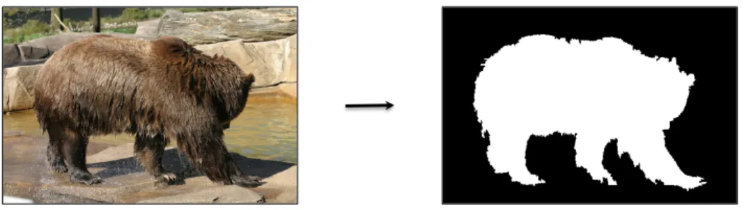
(a) Foreground-background segmentation: given an image, label every pixel as either foreground or background. S" NP" VP" V" NP" N" Det" PP" P" NP" Det" N" elephant" I" shot" an" in" pajamas" my" VP"

I shot an

elephant in my

pajamas

(b) Sentence parsing: given a sentence, create a parse tree representation of the grammatical structure of the sentence.

Figure 1.1: Example Structured Prediction tasks.

task would be to output a parse tree given a sentence [Taskar et al., 2004].

In such problems, exploiting the interdependences between output variables (e.g., the labels of neighboring pixels) leads to superior prediction quality. Thus, SOP seeks to predict all variables jointly. Formally, SOP casts the problem aslearninga mapping from inputs to (structured) outputs

f :_{X → Y}k, (1.1)

where_X is the space of inputs (e.g., images or Chinese sentences) and_Yk is the space of (k-variate and structured) outputs (e.g., image segmentations or English translations of Chinese sentences). Fig. 1.1 provides two examples of SOP tasks.

For Structural Support Vector Machines (Structural SVMs) [Tsochantaridis et al., 2005, Joachims et al., 2009], the mapping is linear and is defined as

f(x;w) = argmax

y∈Yk

(16)

whereψ(x,y)is a joint feature map,ψ:_{X × Y}k_→Rd.1

Finding the maximizingyin (1.2) is known as the MAP (Maximum A Posteriori)inferenceproblem [Koller and Friedman, 2009, Wainwright and Jordan, 2008]. It is always assumed that the score functionwT_ψ₍_x_,_y₎_decomposes.

Otherwise, it would be infeasible to even represent such a function for any interesting problem. For certain decom-positions, there exist exact and efficient methods for MAP inference, however this problem is NP-hard in general [Shimony, 1994].

In Supervised Learning, the mapping f is inferred from labeled data using formulations such as Max-Margin Markov Networks [Taskar et al., 2003], Structural SVMs [Tsochantaridis et al., 2005, Joachims et al., 2009] and Conditional Random Fields (CRFs) [Lafferty et al., 2001]. In these settings one is given training data in the form of input-output pairs

S=_{(xi,yi)} n

i=1 (1.3)

and the goal is to find the weight vectorw in (1.2) that correctly classifies the training pairs,i.e., findwsuch that

yi= argmaxy∈YkwTψ(xi,y).

In the case of Structural SVMS the quality of predictionyˆi=f(xi)is measure by a task-specific loss function

`:_Yk_{× Y}k_→R+, (1.4)

where`(yi,yˆi)denotes the cost of predictingˆyiwhen the correct label isyi. Some examples of loss functions are the

intersection/union criterion used by the PASCAL Visual Object Category Segmentation Challenge [Everingham et al., 2011], and the BLEU score used to evaluate machine translations [Papineni et al., 2002].

Following theEmpirical Risk Minimization(ERM) principle [Vapnik, 1998] the learning formulation for Structural SVMs strives to approximate w∗= argmin w 1 n n X i=1 `(yi, f(xi;w)). (1.5)

This objective is discontinuous and non-convex in w, so surrogate losses are used in practice. Additionally, this learning problem is further complicated for several reasons: First, inference is already computationally intractable. Second, labeled data is expensive and often limited and biased [Torralba and Efros, 2011]. Third, the learning task for SOP is NP-hard in general [David Sontag and Globerson, 2010]. Hence, approximations and other compromises are 1_{In Conditional Random Fields [Lafferty et al., 2001] the}_score_{is normalized to define a probability distribution over outputs}_P₍_y_|_x₎ _∝

(17)

L

i

( ˆ

Y

i

) = min

m

2

[

|

Y

ˆ

i

|

]

`

(

y

i

,

y

ˆ

i

(

m

)

(15)

L

+

i

div

( ˆ

Y

i

) =

L

i

( ˆ

Y

i

) +

↵ `

div

( ˆ

Y

i

)

(16)

`

div

( ˆ

Y

i

) =

M

m<m

0

:

m,m

0

2

[

|

Y

ˆ

i

|

]

⇣

1

(ˆ

y

(

i

m

)

,

y

ˆ

i

(

m

0

)

⌘

(17)

min

W

1

n

X

i

2

[

n

]

L

+

i

div

(

g

(

x

i

;

W

))

(18)

ˆ

Y

i m

=

D

ˆ

y

i

(1)

, . . . ,

y

ˆ

(

i

m

1)

,

y

ˆ

i

(

m

+1)

, . . . ,

y

ˆ

i

(

M

)

E

(19)

ˆ

Y

i

|

y

m

=

D

ˆ

y

(1)

i

, . . . ,

y

ˆ

(

i

m

1)

,

y

,

y

ˆ

i

(

m

+1)

, . . . ,

y

ˆ

i

(

M

)

E

(20)

e.g

.,

L

i

⇣n

·

19

.

56%

,

·

68

.

56%

,

·

5

.

86%

,

·

79

.

00%

o⌘

=

·

5

.

86%

ˆ

Y

i

=

D

·

,

·

,

·

,

·

E

ˆ

Y

i

3

=

D

·

,

·

,

·

E

ˆ

Y

i

|

3

·

=

D

·

,

·

,

·

,

·

E

3

L

i

( ˆ

Y

i

) = min

m

2

[

|

Y

ˆ

i

|

]

`

(

y

i

,

y

ˆ

i

(

m

)

(15)

L

+

i

div

( ˆ

Y

i

) =

L

i

( ˆ

Y

i

) +

↵ `

div

( ˆ

Y

i

)

(16)

`

div

( ˆ

Y

i

) =

M

m<m

0

:

m,m

0

2

[

|

Y

ˆ

i

|

]

⇣

1

(ˆ

y

(

i

m

)

,

y

ˆ

i

(

m

0

)

⌘

(17)

min

W

1

n

X

i

2

[

n

]

L

+

i

div

(

g

(

x

i

;

W

))

(18)

ˆ

Y

i m

=

D

ˆ

y

i

(1)

, . . . ,

y

ˆ

(

i

m

1)

,

y

ˆ

i

(

m

+1)

, . . . ,

y

ˆ

i

(

M

)

E

(19)

ˆ

Y

i

|

y

m

=

D

ˆ

y

i

(1)

, . . . ,

y

ˆ

(

i

m

1)

,

y

,

y

ˆ

i

(

m

+1)

, . . . ,

y

ˆ

i

(

M

)

E

(20)

e.g

.,

L

i

⇣n

·

19

.

56%

,

·

68

.

56%

,

·

5

.

86%

,

·

79

.

00%

o⌘

=

·

5

.

86%

ˆ

Y

i

=

D

·

,

·

,

·

,

·

E

ˆ

Y

i

3

=

D

·

,

·

,

·

E

ˆ

Y

i

|

3

·

=

D

·

,

·

,

·

,

·

E

3

L

i

( ˆ

Y

i

) = min

m

2

[

|

Y

ˆ

i

|

]

`(

y

i

,

y

ˆ

i

(

m

)

(15)

L

+

i

div

( ˆ

Y

i

) =

L

i

( ˆ

Y

i

) +

↵ `

div

( ˆ

Y

i

)

(16)

`

div

( ˆ

Y

i

) =

M

m<m

0

:

m,m

0

2

[

|

Y

ˆ

i

|

]

⇣

1

(ˆ

y

i

(

m

)

,

y

ˆ

(

i

m

0

)

⌘

(17)

min

W

1

n

X

i

2

[

n

]

L

+

i

div

(g(

x

i

;

W

))

(18)

ˆ

Y

i

m

=

D

y

ˆ

i

(1)

, . . . ,

y

ˆ

i

(

m

1)

,

y

ˆ

(

i

m

+1)

, . . . ,

y

ˆ

(

i

M

)

E

(19)

ˆ

Y

i

|

y

m

=

D

y

ˆ

i

(1)

, . . . ,

y

ˆ

i

(

m

1)

,

y

,

y

ˆ

i

(

m

+1)

, . . . ,

y

ˆ

i

(

M

)

E

(20)

e.g

.,

L

i

⇣n

·

19.56%

,

·

68.56%

,

·

5.86%

,

·

79.00%

o⌘

=

·

5.86%

ˆ

Y

i

=

D

·

,

·

,

·

,

·

E

ˆ

Y

i

3

=

D

·

,

·

,

·

E

ˆ

Y

i

|

3

·

=

D

·

,

·

,

·

,

·

E

3

L

i

( ˆ

Y

i

) = min

m

2

[

|

Y

ˆ

i

|

]

`(

y

i

,

y

ˆ

i

(

m

)

(15)

L

+

i

div

( ˆ

Y

i

) =

L

i

( ˆ

Y

i

) +

↵ `

div

( ˆ

Y

i

)

(16)

`

div

( ˆ

Y

i

) =

M

m<m

0

:

m,m

0

2

[

|

Y

ˆ

i

|

]

⇣

1

(ˆ

y

(

i

m

)

,

y

ˆ

i

(

m

0

)

⌘

(17)

min

W

1

n

X

i

2

[

n

]

L

+

i

div

(g(

x

i

;

W

))

(18)

ˆ

Y

i

m

=

D

y

ˆ

(1)

i

, . . . ,

y

ˆ

(

i

m

1)

,

y

ˆ

i

(

m

+1)

, . . . ,

y

ˆ

i

(

M

)

E

(19)

ˆ

Y

i

|

y

m

=

D

y

ˆ

(1)

i

, . . . ,

y

ˆ

(

i

m

1)

,

y

,

y

ˆ

i

(

m

+1)

, . . . ,

y

ˆ

(

i

M

)

E

(20)

e.g

.,

L

i

⇣n

·

19.56%

,

·

68.56%

,

·

5.86%

,

·

79.00%

o⌘

=

·

5.86%

ˆ

Y

i

=

D

·

,

·

,

·

,

·

E

ˆ

Y

i

3

=

D

·

,

·

,

·

E

ˆ

Y

i

|

3

·

=

D

·

,

·

,

·

,

·

E

3

L

i

( ˆ

Y

i

) = min

m

2

[

|

Y

ˆ

i

|

]

`(

y

i

,

y

ˆ

i

(

m

)

(15)

L

+

i

div

( ˆ

Y

i

) =

L

i

( ˆ

Y

i

) +

↵ `

div

( ˆ

Y

i

)

(16)

`

div

( ˆ

Y

i

) =

M

m<m

0

:

m,m

0

2

[

|

Y

ˆ

i

|

]

⇣

1

(ˆ

y

i

(

m

)

,

y

ˆ

(

i

m

0

)

⌘

(17)

min

W

1

n

X

i

2

[

n

]

L

+

i

div

(g

(

x

i

;

W

))

(18)

ˆ

Y

i

m

=

D

y

ˆ

i

(1)

, . . . ,

y

ˆ

i

(

m

1)

,

y

ˆ

(

i

m

+1)

, . . . ,

y

ˆ

(

i

M

)

E

(19)

ˆ

Y

i

|

y

m

=

D

y

ˆ

i

(1)

, . . . ,

y

ˆ

i

(

m

1)

,

y

,

y

ˆ

i

(

m

+1)

, . . . ,

y

ˆ

i

(

M

)

E

(20)

e.g

.,

L

i

⇣n

·

19.56%

,

·

68.56%

,

·

5.86%

,

·

79.00%

o⌘

=

·

5.86%

ˆ

Y

i

=

D

·

,

·

,

·

,

·

E

ˆ

Y

i

3

=

D

·

,

·

,

·

E

ˆ

Y

i

|

3

·

=

D

·

,

·

,

·

,

·

E

3

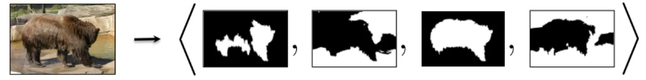
Figure 1.2: Multi-Output Structured Prediction for the foreground-background segmentation task in Fig. 1.1a.

necessary, which translates into limitations and inaccuracies in the models we are able to learn. More details on SOP will be given in Chapter 2.

1.2

Multi-Output Structured Learning

In this thesis we build on the framework of Structural SVMs and propose models that predict fixed-size tuples of structured-outputs

g:_{X → Y}kM, (1.6)

where the input space_Xis as before but where the output space_YkMis onM-tuples2_{of structured-outputs.}

For example, ˆ Yi= D ˆ y(1)_i , . . . ,yˆ_i(M)E (1.7) is anM-tuple of predictions for thei-th input where eachyˆ_i(m) _{∈ Y}k_,_m_{= 1}_{, . . . , M} _{is a structured label,} _e.g_{., a}

segmentation of an image or an English translations of a Chinese sentence. See Fig. 1.2 for an illustration of the idea. Importantly, we develop novel methods to train models such that the multiple predictions in the tuple are comple-mentary ordiversein a sense we formalize shortly.

1.2.1

Insisting on Multiple Predictions

There are, in fact, several reasons behind the benefits of making multiple (diverse) predictions. In this section we provide intuitions from different perspectives for the superiority of Multi-Output Structured Learning:

1. UncertaintyAs noted above, there are numerous reasons for the inadequacy of single MAP solutions. On one end, there is inherent uncertainty in applications due to limited, noisy or, simply, ambiguous observations. On 2_{Our formulation is described with a}_nominal_{ordering of the predictions. However, both the proposed objective function and optimization}

(18)

ˆ

y

(_im)

y

L

+idiv(m)

(ˆ

y

(m) i

; ˆ

Y

i

)

=

8

>

<

>

:

`

i

(ˆ

y

(im)

) +

↵ `

div

( ˆ

Y

i

|

ˆ y(m)_i m

)

if

`

i

(ˆ

y

i(m)

)

<

Li

( ˆ

Y

i m

)

L

i

( ˆ

Y

i m

) +

↵ `

div

( ˆ

Y

i

|

ˆ y(m)_i m

)

otherwise

(21)

min

wm

X

i2[n]

L

+idiv(m)

(ˆ

y

(m) i

; ˆ

Y

i

)

(22)

L

+ilineardiv(m)

(ˆ

y

(m) i

; ˆ

Y

i

) =

`

i

(ˆ

y

i(m)

) +

↵ `

div

( ˆ

Y

i

|

ˆ y(m)_i m

)

(23)

L

+iconstdiv(m)

(ˆ

y

(m) i

; ˆ

Y

i

) =

L

i

( ˆ

Y

i m

) +

↵ `

div

( ˆ

Y

i

|

yˆ (m) i m

)

(24)

I

m

=

n

i

:

`

i(ˆ

y

_i(m)

) =

Li( ˆ

Yi)

o

(25)

min

wm

X

i2Im

L

+ilineardiv(m)

(ˆ

y

(m) i

; ˆ

Yi)

+

X

m0₆=m

X

i2Im0

L

+iconstdiv(m)

(ˆ

y

(m) i

; ˆ

Yi)

(26)

min

wm

2

||

w

m|| 2 2

+

X

i2Im

˜

L

+ilineardiv(m)

(w

m

; ˆ

Y

i

)

+

X

m0₆₌_m

X

i2Im0

˜

L

+iconstdiv(m)

(w

m

; ˆ

Y

i

)

(27)

1

Preliminaries

f

:

X ! Y

k

(1)

score

(y)

f

(x;

w) = argmax

y2Yk

w

T

(x

,

y)

(2)

:

X ⇥ Y

k

!

R

d

(3)

`

:

Y

k

⇥ Y

k

!

R

+

(4)

S

= (x

i

,

y

i

)

|

x

i

2 X

,

y

i

2 Y

k

, i

2

[

n

]

(5)

R

_S`

=

1

n

X

i2[n]

`

(yi

, f

(xi;

w))

(6)

min

w

R

` S

(

f

(

·

;

w)) = min

_w

1

n

X

i2[n]

`

i(

f

(xi;

w))

(7)

2

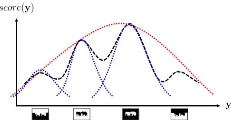
Figure 1.3: Increased expressivity from learning a “portolio” of predictors (blue) compared to a single predictor (red).

another end, the models we are able to learn are necessarily limited and inaccurate, while the inference methods used in practice lack optimality guarantees.

In this work we see multiple-outputs as an effective (or perhaps, necessary) means to manage uncertainty. It is worthy to note that in (unstructured) pattern classification there is a long tradition on building ensembles of classifiers to increase accuracy. See related work in Sec. 1.3.

2. RepresentationalThe methods we develop work by decomposing the input-output mapping. That is, in a spirit akin to mixture models, we propose to decompose a complex input-output mapping into a tuple (or portfo-lio) of simpler input-output mappings that arelocally accurate. As a consequence, our models are indeed a generalization of standard SOP models with superior representational power.

Fig. 1.3 is a caricature of learning a “portfolio” for approximating a multi-modal mapping. If, for the sake of illustration, we picture current methods as uni-modal mappings, then a standard SOP approach would learn a mapping as shown by the red curve while our approach would have as an option the learning a mapping as represented by the blue curves.

3. Statistical[Kuncheva, 2004] offers the following intuition in favor of learning an ensemble of models. Suppose we have a training setS and a set of classifiers C(S)all of which display good performance onS. In such scenario, there is uncertainty as to what the correct single classifier to pick would be. Although the classifiers may be indistinguishable w.r.t. their training performance, they may have differentgeneralizationperformance. Instead of picking a single classifier, a safer option would be to use all ofC(S)and “average” their outputs. This ensemble classifier may not be better than the single best classifier inC(S)but can eliminate the risk of picking an inadequate single classifier (based on training error).

A different intuition on the benefit of averaging predictors from [Hastie et al., 2009] is as follows. In a regression setting we are given a set of input-output pairs_{(Xi, Yi)}

n

i=1whereXi ∈Rp andYi ∈R, and seek to find a

(19)

mappingfˆ:Rp

→Rso as to minimize the squared error _n1

n P i=1 Yi−fˆ(Xi) 2 .

If we assume thatY=f(X) +whereE[] = 0andVar[] =σ2, we can derive the following expression for the expected prediction error of regression fitfˆ(X)at input pointX=x0

Err(x0) = E[Y −fˆ(x0)|X=x0]

=σ2+ (E[ ˆf(x0)]−f(x0))2+ E[ ˆf(x0)−E[ ˆf(x0]]2

=σ2+ Bias2[ ˆf(x0)] + Var[ ˆf(x0)]

=Irreducible error+Bias2+Variance. (1.8)

Thus, prediction error may be reduced by,e.g., decreasing Bias while keeping Variance constant or vice versa. Typically, the more complex we make a modelfˆthe lower the Bias but the higher the Variance.

An average of M i.i.d. random variables each with varianceσ2 _{has variance} 1

Mσ

2_{. Hence, some ensemble}

methods (e.g., bagging, random forests) seek to reduce the expected prediction error by reducing variance while keeping bias approximately constant.

When learning multiple models from the same training data the i.i.d. assumption will not hold in general. If the variables are simply i.d. (identically distributed but not necessarily independent) with positive pairwise correlationρ, the variance of the average is

ρ σ2+1−ρ

M σ

2_.

(1.9)

Thus, the expected prediction error can be reduced by averaging multiple models while reducing the correla-tion between the models in the ensemble. Bootstrapping seeks to achieve decreased correlacorrela-tion via randomly sampling train data while,e.g., random forests seek a decrease in correlation through random selection of input variables during the tree-growing process.

4. ComputationalWhen usingdescentmethods to optimize a non-convex objective there is a risk of getting stuck in poor local optima. This is often the case in learning and inference methods for SOP [Globerson and Jaakkola, 2007, Meshi et al., 2010]. Learning multipleuncorrelatedmodels is a means to mitigate against such difficulties. At train-time this objective will increase our chances of finding good models or good (locally accurate) model portfolios. As a result, during test-time, we should have increased chances of finding good predictions.

(20)

1.2.2

Cascaded Architectures

A popular approach to dealing with increasingly complex models is that ofdecomposition. In general, decomposition approaches (e.g., [Komodakis et al., 2011, Sapp et al., 2011, Koo et al., 2010]) split the model into an ensemble of tractable models and enforce various degrees of agreement constraints on the decisions derived from the sub-models. An important form of decomposition, that deviates from the probabilistic framework, is that of feed-forward pipelines which propagate (sub-optimal) decisions (e.g., in Structured Prediction [Weiss and Taskar, 2010, Sapp et al., 2010, 2011]).

This thesis is part of a body of work that suggests an approach that leverages aspects of both compromises noted above. Namely, this work suggests cascaded architectures with two types of stages:

Type 1 Efficient Multi-Output Structured Modelsare probabilistic models that, while tractable, are capable of taking a doubly-exponential search-space and pruning it drastically. The output of these models should be a (relatively) small set of high-quality hypotheses with high coverageor recall, e.g., a set of DiverseM-Best Hypotheses.

Type 2 Consumers of Multiple Hypothesescome in different forms. Re-rankersare models able to rank a small set of hypotheses perhaps by taking advantage of interactions that are too complex (e.g., high-order features) to be used for inference in the original search-space or by using other forms of information available at test-time. For instance, in Computer Vision, this is the case for state-of-the-art methods for human-pose estimation in video which produce multiple predictions at every frame and then compute a track by smoothing the transitions over the entire sequence using dynamic programming [Park and Ramanan, 2011, Batra et al., 2012]. In Natural Language Processing, this is the case for sentence parsing [Collins, 2000], Semantic Role Labeling [Charniak and Johnson, 2005, Toutanova et al., 2005] and Machine Translation [Shen et al., 2004], where an initial system produces a list ofM-Best hypotheses [Huang and Chiang, 2005, Pauls et al., 2010] (also calledk-best lists in the NLP literature), which are subsequently re-ranked.

Additionally, as suggested earlier, multiple hypotheses may serve as initializations forsubsequent optimization or validation. This is particularly interesting when subsequent optimization or validation is costly,e.g., visual inspection, simulation or experimentation in the real-world. An example of subsequent optimization is the system developed in Chapter 5 for camera relocalization, and an example of costly simulation can be found in protein design applications [Fromer and Yanover, 2009].

Aggregatorsare models capable of combining multiple hypotheses. For example, in human-pose estimation temporal smoothing could be used not only to re-rank complete poses but to combine poses at the level of parts. In the end-to-end system of Chapter 5 a different form of hypothesis aggregation is shown to introduce accuracy

(21)

improvements.

In this category, we also include the user portion ofInteractive Systemswhere the goal is to produce hypothe-ses for an expert or user in the loop. Popular examples include tools for interactive image segmentation (where the system produces a cutout of an object from a picture [Boykov and Jolly, 2001, Rother et al., 2004]); systems for image processing/manipulation tasks such as image denoising and deblurring (e.g., Photoshop); or machine translation services (e.g., Google Translate). These problems are typically modeled using structured probabilis-tic models and involve computing the MAP solution. In order to minimize user interactions, these systems could present the user not only a single prediction but a small set of diverse predictions, and simply let the user pick the best one.

In this thesis, Chapters 3 and 4 developType 1models while Chapter 5 develops a full (end-to-end) system withType 1andType 2components.

Finally, another form of cascaded architecture lies in the investigation of energy functions, learning methods and application-specific matters. It has been argued [Fromer and Yanover, 2009, Chen et al., 2013] that the statistical analysis of multiple solutions is beneficial in acquiring insight as to the appropriateness of energy functions used in practice; the effects of training data (e.g., w.r.t. train data size and noise); and in understanding and characterizing salient aspects of good quality solutions.

1.2.3

Diversity

In this work we speak of diversity in sets of multiple predictions. Formally, we assume the availability of a distance or dissimilarity function between pairs of predictions,e.g.,∆(y,y0). Equipped with such function, we may compare the relative diversity of different pairs of hypotheses,i.e., where higher values of dissimilarity are deemed more diverse.

To extend the notion of diversity to tuples (as in (1.7)) of more than two outputs we aggregate measures of pairwise dissimilarity over all pairs in the tuple,

∆( ˆYi) = M m<m0: ˆ y_i(m),ˆy_i(m0)∈_Yˆ_i ∆(ˆy(_im),yˆ_i(m0)), (1.10)

whereLis an aggregation operator such asmeanormin.

Insisting on diversity is a mechanism for decreasing correlation in the predictions (and predictors), which is nec-essary for learning classifiers that make complementary mistakes. Striving for diversity when generating multiple solutions is important to the following objectives:

(22)

2010].

2. Maximize information gain,e.g., sensor placement [Krause et al., 2006].

3. Covering the most interesting or important cases,e.g., summarizing a news story by selecting a subset of sen-tences that include all relevant facts [Gillenwater et al., 2012, Ross et al., 2013].

4. Summarize a configuration space through representative cases, e.g., in interactive systems or when tracking people in video [Batra et al., 2012, Park and Ramanan, 2011].

5. Increase efficiency by avoiding wasted computation on redundant solutions,e.g., this thesis, [Batra et al., 2012, Kulesza and Taskar, 2012, Slivkins et al., 2013].

1.2.4

Set min-loss

In this thesis we take an ERM approach as in standard SOP. However, we argue that in Multi-Output Structured Learning, the right loss to minimize during training is the “setmin-loss”

Li( ˆYi) = min

ˆ

y∈_Yˆ_i`(yi,yˆ), (1.11)

where`(_·,_·)is the traditional task-loss from standard SOP andyi is the ground-truth solution. That is, a tupleYˆiis

penalized only for the error in the most accurate prediction it contains.

The setmin-loss is so central to our developments that we train all of our multi-output SOP systems to minimize this loss. It has the following properties:

1. It allows predictions to be diverse. While the loss itself does not enforce diversity, it does not place any restric-tions on it. We will see that within the ERM framework the setmin-loss is able to produce decreased correlation in a similar (but superior) way as bootstraping samples decreases correlation in,e.g., bagging.

2. Applies to standard SOP datasets containing single labels. This enables our methods to learn from exactly the same datasets as regular SOP methods do.

Note that replacing the set min-loss with other aggregate losses would have drastically different effects. For instance, the setmax-loss would prevent diversity (thus, increasing correlation) and lead to decreased performance. Even the setmean-loss would limit diversity, which is crucial to the success of our approach.

The use of the setmin-loss sets our work apart from all previous work in SOP. In certain contexts aggregate losses with similar signature have appeared. However, we do not know of any previous SOP work on learning to minimize the setmin-loss.

(23)

e.g., [Cesa-Bianchi and Lugosi, 2006]. In this literature the problem setting (e.g., sequence prediction) and output spaces are different. Yet, there is a connection between our objective to minimize the setmin-loss and their objective to minimize regret, which deserves attention.

1.3

Related work

1.3.1

Producing Multiple Structured-Outputs

A standard way of producing multiple structured predictions in probabilistic models is to find the topMmost probable (or high-scoring) configurations for a scoring function like in (1.2) (normalization is of no concern in these settings). This problem is known in the literature as the M-Best MAP problem and M-Best versions of most standard MAP inference methods have been developed: max-flow [Nilsson, 1998], Loopy Belief Propagation [Yanover and Weiss, 2003], Linear Programming relaxations [Fromer and Globerson, 2009, Batra, 2012], Sampling [Porway and Zhu, 2011] and Search [Andres et al., 2012].

There are at least three problems with M-Best MAP approaches:

1. The multiple solutions found tend to be redundant, offering little benefit (e.g., additional or complementary information) w.r.t. each other. As a consequence many solutions need to be generated before achieving any significant gain.

2. The approaches exhibit a train-test inconsistency. Models are trained to produce single-outputs,i.e., to match the single-label data distribution (Maximum Likelihood) or to score single-label ground-truth the highest by a margin (Maximum Margin). However, models are used at test-time to produce multiple outputs.

3. All approaches are computationally expensive. In general, solutions are computed sequentially by constrain-ing the original scorconstrain-ing function so that previously found solutions are eliminated. This, compounded with redundancy, severely limits the applicability of M-Best MAP approaches.

Compared to M-Best MAP approaches the methods in this thesis are advantageous because: 1. The solutions produced by our methods are complementary (or diverse) by design.

2. Train and test procedures are consistent,i.e., the models we propose are designed and trained for making multi-ple predictions.

3. MAP inference with our models is not sequential and is as efficient as standard MAP inference (up to a constant factor).

4. Since our models are effectively ensembles of structured models, their representational power is increased w.r.t. traditional models as was argued above. As a consequence the predicted tuples contain hypotheses of higher

(24)

accuracy than those produced by single output models.

There are also approaches that compound M-Best MAP inference so as to attain diversity in the multiple solutions. Non-Maximum Suppression (NMS) [Felzenszwalb et al., 2010, Blaschko, 2011, Park and Ramanan, 2011] works by generating a large set of M-Best solutions and then discarding redundant solutions. Thus, while diversity may be attained through NMS, there is still a need to generate and evaluate many redundant solutions using M-Best MAP approaches. Hence, the methods in this thesis are superior in senses 2 to 4 above w.r.t. to NMS.

Another method that was recently proposed is Diverse M-Best MAP [Batra et al., 2012]. This is a sequential ap-proach to obtaining multiplediversesolutions that works by first computing the MAP solution and next, compounding the original scoring function with a linear term penalizing configurations for their closeness to solutions previously found. This method is more computationally efficient compared to NMS but, similarly to NMS, falls short w.r.t. the methods in this thesis in senses 2 to 4 above. Indeed, our experimental evaluation will show that the solutions found with the methods in these thesis are of superior quality than those found using Diverse M-Best MAP.

The M-Modes problem for graphical models was recently introduced by [Chen et al., 2013]. In this setting the problem is to predict the M configurations of highest probability that, at the same time, are local maxima of the probability landscape (the authors define the notion of local maximum for discrete output spaces with the aid of a distance function on configurations). Modes are intrinsically diverse but the methods proposed are sequential and work only for low treewidth models.

Variational Methods [Wainwright and Jordan, 2008] could also be used to decompose a SOP model and make multiple predictions more efficiently. The main issue with this direction is that the method would work to approximate an incorrectly estimated model and will introduce additional assumptions to factor the distribution. The methods in this thesis work in the opposite order: a complex distribution is decomposed first and then each (local) component is estimated from data.

Structured Determinantal Point Processes (SDPPs) [Kulesza and Taskar, 2010, 2012] combine SOP models with Determinantal Point Processes (DPPs) [Macchi, 1975] to enforce diversity in structured-output predictions. Currently, the main limitations of SDPPs are that they have only been specified for low treewidth SOP models and that inference is done sequentially via sampling. Further, to our knowledge no work has shown how to learn SDPPs from labeled data.

The work of [Lampert, 2011] on Multi-Label Structured Prediction (MLSP) is also on predicting sets of structured labels. However, the motivation and setting of that work is fundamentally different from ours. MLSP addresses the problem of predicting all true labels for an instance (such as all object classes present in an image). In contrast, our models propose a set of structured labels at least one of which is close to the single ground-truth label for the instance.

(25)

Further, MLSP requires ground-truth set outputs to train from, which we do not. In fact, our developments and MLSP are orthogonal approaches, e.g., we could introduce MLSP within our framework to learn to predict multiple and diversesets of structured-outputs (e.g., multiple guesses by the algorithm where each guess is a set of bounding boxes for the objects in an image).

1.3.2

Ensemble Learning (Combining Classifiers)

At a high-level, the motivation for our developments is similar to that of a long tradition of work on ensemble learning for unstructured spaces. In this context, Hastie et al. [2009] state:

“In terms of basis functions, we want a collection that covers the space well in places where they are needed, and are sufficiently different from each other for the post-processor to be effective.”

Besides the structural aspect, our methods are different from traditional ensemble methods in the following senses: 1. We choose to remain agnostic about the relative importance of each predictor.

2. We do not immediately “average” predictors or combine outputs. In particular, we do not seek to learn a combination strategy from training data but insist to use additional information available at test-time to carry out further processing and eventually combination or re-ranking of multiple hypotheses.

3. Armed with the setmin-loss we are able to discover domains (or regions of competence) and achieve diversity. We provide further elaboration on this in the Multi-Task Learning discussion below.

Here is a brief overview of some of the approaches developed in this tradition:

1. Mixture models combine multiple distributions probabilistically for increased representation power. For in-stance, a mixture of Gaussians may approximate a multi-modal distribution much better than a single (uni-modal) Gaussian, P(x_|π,µ,Σ) = M X i=1 πiN(x;µi,Σi). (1.12)

2. Mixture of experts increase the capability of mixture models by allowing the mixing coefficients to be functions of the input variable,

P(x_|π,µ,Σ) =

M

X

i=1

πi(x)N(x;µi,Σi). (1.13)

3. Classifier Selection is motivated by the idea ofregions of competenceand assumes it is possible to determine the competence of each classifier in the ensemble for a given input. This is similar to theπi(x)coefficients in

(26)

classifier to make the classification of the input.

The idea of using different classifiers for different inputs goes, at least, back to [Dasarathy and Sheela, 1979]. 4. Bayesian model averaging considers a set of candidate models_Mm,m=1, . . . , M(which may be of the same

or of different types,e.g., neural networks and regression trees) for a training setS=_{(xi, yi)} n

i=1. Supposeζ

is a quantity of interest,e.g., a predictionf(x)at fixed inputx. Then the posterior distribution ofζis

P(ζ_|S) =

M

X

i=1

P(ζ_|Mm, S)P(Mm|S), (1.14)

with posterior mean

E(ζ_|S) =

M

X

i=1

E[ζ_|Mm, S]P(Mm|S). (1.15)

This Bayesian prediction is thus a weighted average of the individual predictions, with weights proportional to the posterior probability of each model.

This formulation leads to different model averaging strategies:

(a) Committee methods use unweighted averages. In,e.g., Bagging (or Bootstrap aggregation) the models are fit on different bootstrap samples of the training data to reduce correlation (and variance).

(b) The Bayesian Information Criterion (BIC) is often used to approximate posterior model probabilities. (c) In Stacking, a leave-one-out strategy is used to determine weights. Letfˆm−i(x)be the prediction atxusing

modelmapplied to the dataset with thei-th observation removed. For,e.g., least squares linear regression the stacking weights are given by

ˆ w= argmin w n X i=1 " yi− M X m=1 wmfˆm−i(xi) # . (1.16)

The final predictor is then

M

P

m=1

ˆ

wmfˆm(x).

5. Boosting applies a classification algorithm sequentially toweightedversions of training data. It thus produces a sequence of classifiersGm(x),m=1, . . . , Mwhose predictions are to be combined through a weighted majority

vote to produce the final prediction

G(x) = sign M X m=1 αmGm(x) ! . (1.17)

(27)

classifier Gm−1 have their weights increased, while those which were correctly classified have their weights

decreased. As iterations proceed, samples that are found difficult to classify achieve ever-increasing influence. Thus, classifiers are forced to concentrate on those training samples that aren’t properly handled by previous classifiers.

6. Random Forests is a modification of bagging for building a large collection ofde-correlated trees. The key idea in random forests is to improve on the variance reduction of bagging by reducing correlation between trees, without increasing the variance too much. This is achieved in the tree-growing process through a random selection of a subset of the input variables as candidates for splitting.

7. Neural Networks may be also be regarded as an ensemble method that simultaneously learn the parameters of the hidden units, along with how to combine them.

8. Support Vector Machines can also be regarded as an ensemble method performingL2regularized model fitting in

high-dimensional feature spaces. A step further is taken in the Multiple Kernel Learning framework [Lanckriet et al., 2004, Bach et al., 2004] where the kernel is expressed as a convex combination of elements of a finite set, which is learned from data.

1.3.3

Domain Adaptation and Multi-Task Learning

According to [Caruana, 1997], Multitask Learning (MTL) is an inductive transfer mechanism whose principle goal is to improve generalization performance. MTL improves generalization by leveraging thedomain-specificinformation contained in the training signals of related tasks. This is accomplished by training tasks in parallel while using a shared representation.

A distinction between Domain Adaptation (DA) and MTL has been made in the literature [Daum´e III, 2009] though this is not always maintained. In DA the problem is to learn multiple classifiers for solving the same task ondata from different distributions; while in MTL, the problem is to learn multiple classifiers for solving different tasks overdata from the same distribution. Both, Domain Adaptation (DA) [Blitzer et al., 2006, Ben-David et al., 2006, Daum´e III, 2007] and Multi-Task Learning (MTL) [Caruana, 1997, Bickel et al., 2007], involve learning related hypotheses on multipledatasets.

Importantly, the MTL literature has noted the importance of avoiding negative transfer: Sharing information between two unrelated tasks can worsen performance on both tasks [Daum´e III, 2009, Kumar and Daum´e III, 2012].

Two insights from Multi-Task learning are relevant and supportive of the work in this thesis: 1. In general, to different domains correspond different best-performing classifiers.

(28)

can be exploited but one must prevent negative transfer.

In MTL the existence of multipledomainsis assumed. Additionally, it is also assumed that the domains for all train and test examples are known a priori. The methods in this thesis may also be regarded as making a multiple domain assumption. However, in this work the domains are not known a priori. Hence, the use of the setmin-loss in this thesis can be seen as a means to discover domains within the training data, which provides justification for learning different classifiers for the different domains.

To recapitulate, the methods we propose are motivated similarly to traditional ensemble methods but, similarly to multi-task learning, are domain-aware. Thus, unlike standard ensemble methods which use,e.g., randomization to decrease correlation, our methods discover domains and attain decreased correlation through domain specialization.

1.3.4

Multi-label Prediction

In unstructured output spaces, multi-label prediction is a generalization of multi-class prediction where an input object may be associated with any (finite) number of outputs. For instance, the multiple labels could effectively represent different classification tasks or,e.g., in computer vision applications the multiple labels could correspond to multiple instances of a classification or detection task (consider detecting multiple objects of the same class in an image).

Different techniques for multi-label prediction are available which formulate the problem, e.g., as multi-class classification by treating every possible label subset as a class of its own [Boutell et al., 2004]; as a collection of classifiers each making an independent prediction for one of the labels [Joachims, 1998]; as a ranking problem by learning a function for ranking all potential labels [Schapire and Singer, 2000]; or as a structured-prediction task for jointly predicting a set of labels [Yue et al., 2007, Yue and Joachims, 2008].

Besides the lack of structure in the individual labels, multi-label prediction differs from the work in this thesis in the rationale and meaning of the multiple labels. Namely, in this work the multiple labels are different hypotheses for a single instance of a single predictive task. As mentioned in Sec. 1.3.1, there is one previous work on Multi-Label Structured Prediction.

1.3.5

Diversity

The Information Retrieval community has been exploring diversification of results for,e.g., Web search or document summarization applications. [Carbonell and Goldstein, 1998] proposed Maximal Marginal Relevance, a non-learning algorithm for obtaining a diverse ranking from a non-diverse ranking. Critically, their approach assumes access to a relevance function and a pairwise (document) similarity function.

(29)

Joachims, 2008] the output is a ranking of search results where the output structure serves to enforce diversity. This is in contrast to our methods where each label is structured but where we are able to forgo having any structure on the tuple of structured labels. [Raman et al., 2012] develop an algorithm for learning both relevance and the desired amount of diversity from set-valued preference data that can be derived from implicit feedback.

Often, the task has been cast as an online learning problem,e.g., [Radlinski et al., 2008] propose two online learning algorithms that directly learn a diverse ranking of documents based on user clicking behaviors. Their Multi-Armed Bandit (MAB) [Cesa-Bianchi and Lugosi, 2006] algorithms simulate greedy strategies for maximizing a submodular set function.

[Slivkins et al., 2013] initiate the study of bandit learning-to-rank with side information on similarity between documents. They consider a MAB setting where the arms form a metric space providing information on the similarity between arms and where the goal is to minimize query abandonment. In this setting an algorithm may make inferences about similar arms without exploring them.

The work of [Eban et al., 2012] on multi-class sequence prediction proposes to minimize the “hindsight loss” which is equivalent to the setmin-loss for sequences of multi-class labels. Besides the multi-class aspect, their work learns to make predictions from sequences and not single ground-truth as we do. Yet, they arrive at a learning formulation similar to that in Chapter 3.

1.3.6

Submodularity

A reward set-functionf :_{S →}Ris said to be submodular if it obeys the following property:

For any setsS1, S2⊆ S, and elements∈ S,f(S1∪ {s})−f(S1)≤f(S1∪S2∪ {s})−f(S1∪S2).

Intuitively, submodularity captures the notion of diminishing returns: adding an element to a large set increases the reward less than adding the same element to a smaller set. Turns out that submodularity is sufficient for polynomial-time minimization of rewardf [Gr¨otschel et al., 1981]. However, maximization is NP-hard in general but there are constant-factor approximation algorithms for the case of non-negativef, [Feige et al., 2011].

A set-functionf is said to be monotone if for any setsS1, S2,f(S1) ≤ f(S1∪S2)andf(S2)≤ f(S1∪S2).

Intuitively, adding more elements to a set will never hurt. If a reward functionf satisfies monotonicity in addition to submodularity, then maximization via a greedy strategy gives a constant factor approximation of(1₋1_e), [Nemhauser et al., 1978].

The general problem of learning to optimize submodular reward functions from data has become increasingly important in Machine Learning due to its various application areas, e.g., result diversification, summarization, set cover (sensor placement), cut functions (attractive MRFs), and inferring diffusion networks [Krauze and Guestrin].

(30)

There are two broad approaches to address this problem:

1. Learn a model that matches the submodular rewards displayed in training instances. Then use this model to make new predictions, e.g., [Yue and Joachims, 2008, Raman et al., 2012] and work on DPPs [Kulesza and Taskar, 2012] fall in this category.

2. Imitation learning approaches where list prediction is decomposed into a sequence of simpler tasks. The en-semble of tasks seeks to mimic the greedy strategy to submodular function optimization. [Streeter and Golovin, 2008, Streeter et al., 2009, Radlinski et al., 2008, Dey et al., 2012, Slivkins et al., 2013, Ross et al., 2013] fall in this category.

The (negated) setmin-loss used in this work is both monotone and submodular. Hence, imitation learning ap-proaches for approximating greedy strategies to submodular function maximization would likely be successful within our framework. While we do not pursue this direction explicitly in this thesis, future work should elucidate the rela-tionship between the methods in this thesis and the theories of online learning and submodular fuction optimization.

1.4

Summary of Contributions

1. We introduce Multi-Output Structured Learning and Empirical Risk Minimization with the setmin-loss (Chapter 3).

In this chapter we address the problem of generating multiple hypotheses for structured prediction tasks in the context of cascaded architectures or interactive systems. In such settings it is beneficial to generate multiple hypotheses and pass those along for further optimization; as input to increasingly complex tasks; or for selection or aggregation when additional information is available at test-time.

The standard approach for h