Scuola di Scienze
Dipartimento di Fisica e Astronomia Corso di Laurea Magistrale in Fisica
WISDoM: Wishart Distributed Matrices
Multiple Order Classification.
Definition and Application to fMRI
Resting State Data.
Relatore:
Dott. Enrico Giampieri
Correlatore:
Prof. Daniel Remondini
Presentata da:
Carlo Mengucci
Abstract iii
Introduction v
1 An Introduction to Brain Imaging 1
1.1 The resting State . . . 1
1.1.1 Earlier Studies . . . 1
1.1.2 The Resting State in Brain Disease . . . 4
1.2 Investigating the Resting State . . . 7
1.2.1 The fMRI Technique . . . 7
1.2.2 The BOLD Signal . . . 9
1.2.3 Data Preprocessing . . . 13
1.2.4 The Functional Connectivity Matrix . . . 15
2 The Wishart Distribution 17 2.1 Definition . . . 17
2.2 PDF Computation for Invertible Σ . . . 18
2.2.1 Visualizing the Wishart Distribution . . . 18
2.3 The Wishart Distribution in Bayesian Conjugate Prior Analysis 20 2.3.1 Bayesian Inference and Priors Distributions . . . 20
2.3.2 The Wishart Conjugate Prior . . . 21
3 The WISDoM Multiple Order Classification 25 3.1 Wishart Sampling . . . 25
3.1.1 Computing the Estimated Distribution . . . 26
3.2 Log-Likelihood Ratio Measure . . . 28
3.2.1 Complete Matrix Measure . . . 29
3.2.2 Single Feature Measure and Multiple Order Reduction 29 3.2.3 Generalizing to (p−n) Order Transformations . . . 32
3.3 Pipeline . . . 33
3.3.1 The Snakemake Environment . . . 34 i
3.3.2 The WISDoM Pipeline . . . 36 3.3.3 Classification Methods . . . 39
4 Results of The WISDoM Multiple Order Classification 45
4.1 The ADNI2 Database: Study and Results . . . 46 4.1.1 Data Exploration and Selection for WISDoM
Classifi-cation . . . 47 4.1.2 Results . . . 50
Conclusions 61
In this work we introduce the Wishart Distributed Matrices Multiple Or-der Classification (WISDoM) method. The WISDoM Classification method
consists of a pipeline for single feature analysis, supervised learning, cross validation and classification for any problems whose elements can be tied to
a symmetric positive-definite matrix representation. The general idea is for informations about properties of a certain system contained in a symmetric positive-definite matrix representation (i.e covariance and correlation matri-ces) to be extracted by modelling an estimated distribution for the expected classes of a given problem.
The application to fMRI data classification and clustering processing fol-lows naturally: the WISDoM classification method has been tested on the ADNI2 (Alzheimer’s Disease Neuroimaging Initiative) database. The goal was to achieve good classification performances between Alzheimer’s Dis-ease diagnosed patients (AD) and Normal Control (NC) subjects, while re-taining informations on which features were the most informative decision-wise. In our work, the informations about topological properties contained in ADNI2 functional correlation matrices are extracted by modelling an es-timated Wishart distribution for the expected diagnostical groups AD and NC, and allowed a complete separation between the two groups.
In recent years, the interest of the scientific community on brain interactions modelling has greatly increased. The advent of the fMRIfunctional magnetic resonance imaging technique, a non-invasive procedure which provides good
balance between temporal and spatial resolution, has opened an entire new field of anatomical and functional analyses. The discovery of the importance of theresting state of the brain, which is far from being characterised by the
mere statiscal noise of an unperturbed system, togheter with the discovery of the Default Mode Networks, has brought forth several new questions about the underlying mechanisms of human cognition. Studying the resting state is impossible with the traditional subtraction technique, therefore new methods have been implemented.
The use of graph theory to model the brain topological and
dynami-cal properties, based on Functional Correlation Matrix analysis, has also
achieved great results. Comparative studies of different brain disorders diag-nosed subjects, have highlighted the role of different default mode networks in global and local information processing capacity. The characteristic dis-ruption of topological properties induced by brain disorders takes on a de-cisive role in brain region landmarking, thus offering a great possibility for preventive diagnostic and classification studies.
As a matter of fact, these type of analyses are all bound to undergo ceratin issues tied to the processing of high-throughput data. The usual high dimension of functional correlation matrices may indeed lead to convergence problems in Liner Discriminant Analysis or Principal Component Analyisis based methods, preventing an efficient feature selection from being obtained. On the other end, with the ever increasing computational power available, machine learning and heuristic statistical methods like the one introduced in this work, can be of great help in feature selection and classification perfor-mance enhancement. In our work, the informations about topological prop-erties contained in functional correlation matrices are extracted by modelling
an estimated distribution for the expected classes of a given problem. Specif-ically, a Wishart distribution for symmetric positive-definite matrices is used, being his probability density function of closed algebraic form. Furthermore, algebraic properties of symmetric positive-definite matrices are taken into account in order to define single feature transformations. The features are transformed according to the weight they are assigned in assessing the clas-sification decision, with respect to one class or another. Doing so, we gain informations about a feature’s significativity in characterizing the correlation properties of a system.
The methdod introduced in this work, the Wishart Distributed Matrices Multiple Order Classification, consists of a pipeline for single feature
analy-sis, cross validation and classification for any problems whose elements can be tied to a symmetric positive-definite matrix representation. The applica-tion to fMRI data classificaapplica-tion and clustering processing follows naturally, it has indeed been tested on the ADNI2 (Alzheimer’s Disease Neuroimag-ing Initiative) database. The goal was to achieve good classification perfor-mances between Alzheimer’s Disease diagnosed patients (AD) and Normal Control (NC) subjects, while retaining informations on which features were the most informative decision-wise. In this way, informations about signi-ficative anatomical areas and underlying structure might be extracted.
This work is structured as follows:
• Chapter 1: the state of art of fMRI resting state studies is presented,
while an overview on MRI physical bases are also outlined. An overview on the importance of the default mode networks’ properties in brain disease studies is presented, then the physics of Blood Oxygen Signal is defined. The final part of the chapter is an excursus on the most com-mon data preprocessing procedures and the computation of Functional Correlation Marices.
• Chapter 2: the Wishart distribution and its applications are defined.
A closed probability density function for the symmetric positive-definite matrices case is derived. The importance of the Wishart distribution in Bayesian conjugate prior analysis is then outlined.
• Chapter 3: The WISDoM Multiple Order Classification Method is
described in both an analytical and technical way. Feature transfor-mation based on symmetric positive-definite matrices’ properties are defined. A generalization for different orders of said transformations is then derived. The general implemented. pipeline and the Snake-Make environment are then presented and described. The final section
of the chapter is an overview on possible classification and clustering methods, to be used on the Snakemake section of the pipeline outputs. • Chapter 4: The ADNI2 study is presented and classification and
clus-tering results are discussed. A network growth approach is also pre-sented for comparison purposes.
An Introduction to Brain Imaging
In this section, a resume of different important aspects in brain modelling and imaging is presented. Starting from an overview onresting state studies, the
importance of the study of thedeafult mode network is underlined especially
as far as the disruption of its topological and dynamical properties in several forms of brain disease are concerned.
Then, an introduction to fMRI and BOLD signal analysis techniques is
made in order to define the framework of the data used to train the model proposed to solve the classification problem treated in this thesis.
1.1
The resting State
1.1.1
Earlier Studies
Many definitions have been brought forth as far as brain’s resting state is concerned [4]: a sign of the increasing interest of the scientific community over the years, after the obsversations of its properties. As a matter of facts, unlike the equilibrium state of an unperturbed noisy physical system, the spontaneous state of the brain does not show a meaningless random activity, as expected by the scientists until two decades ago. Since the early studies of cerebral metabolism it has been noted that, although the human brain amounts to just 2% of the total body mass, it consumes 20% of the body’s energy; these meaurements were made over brains in resting state.
This has led to asking a crucial question: whether cerebral metabolism 1
changes globally when one goes from a quiet rest state to performing a chal-lenging arithmetic problem. Surprisingly, metabolism remained constant; the local changes were too small (usually less than 5% compared with the resting energy consumption) to be detected by methods designed to measure the energy consumption of the brain as a whole [1]. For several years though, spontaneous brain activity has been systematically overlooked.
As a matter of facts, neuroimaging practices were largely based on the assumption that ongoing activity is sufficiently random and can be averaged out in statistical analysis. As all the efforts of the scientific community were focused on understanding cognitive behaviour, scans of resting state brain activity were often acquired across these studies for mere control compari-son and noise averaging practices, but researchers routinely began noticing that some brain regions showed more activity in resting state condition than during the execution of tasks.
A major step in defining the importance of resting state’s studies has been made by the series of pubblication of Raichle, Gusnard and collagues in 2001 [2]. In this study they isolate a set of brain regions, the Default Mode Network (DMN), characterized by surprisingly high metabolic rate during
rest, and, on the other hand, by the greatest deactivation during externally imposed cognitive tasks. Their work propose that DMN is to be studied as a foundamental neurobiological system, like the motor system or the visual system. It contains a set of interacting brain areas that aretightly functionally connected and distinct from other systems within the brain.
An example of DMN anatomy studied via BOLD (blood oxygen level dependant) signal is shown in fig.(1.1).
After this discovery, other patterns of activities were found, leading to the definition of many resting state networks (RSNs) [4].
Different RSNs found by subsequent studies are visible in figure(1.2). The resting state can thus be defined as a cognitive state in which a subject is quietly awake and alert but does not engage in any specific cognitive or behavioural task [5].
Figure 1.1: Regions of a single subject’s brain that are correlated (positive values) and anticorrelated (negative values) during resting fixation in a func-tional MRI study. Source: Fox et al (2005). [3]
Figure 1.2: Different Resting State Networks found in literature and summa-rized by Van Den Heuvel et colleagues, 2010 [4]
1.1.2
The Resting State in Brain Disease
Most, if not all, physiological and psychiatric diseases have been found to have disrupted large-scale functional and/or structural properties. This fact opens a wide array of possibilities as far as characterization, modelling and predictive studies are concerned for different types of disease. Disorders like autism, schizophrenia and Alzheimer’s disease have all been correlated to resting state network’s alterations.
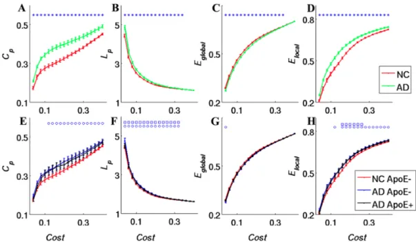
In example, Alzheimer’s disesase diagnosed subjects have been found to have enhanced local network properties while having disrupted global prop-erties with respect to non-diagnosed subjects [6]. Results of these type, based on the observations of altered topological properties of functional networks, are shown in fig.(1.3).
Figure 1.3: Change of network parameters as a function of connection density (Cost). Clustering coefficient (A), shortest path length (B), global efficiency (C) and local efficiency (D) of the Alzheimer’s Disease (green line) and Nor-mal Control (red line) groups as a function of Cost. Clustering coefficient (E), shortest path length (F), global efficiency (G) and local efficiency (H) of the AD ApoE4+ (black line), AD ApoE4- (blue line) and NC ApoE4- (red line) groups as a function of Cost. The error bars correspond to the standard error of the mean. Source: Xiaohu Zhao , Yong Liu et al. 2012 [6]
We can see that clustering coefficients, the shortest path length, local ef-ficiency, and connection density are all enhanced in Alzheimer’s disease
di-agnosed patients, whereas global efficiency is lower. As a matter of fact,
Cp is a measure of local network connectivity: it reflects the local efficiency
and error tolerance of a network. Higher network clustering coefficients in-dicate more concentrated clustering of local connections and stronger local information processing capacity [5]. TheCp of brain functional networks was
found to be higher in Alzheimer’s disease diagnosed patients, indicating that these patients have stronger local information processing capacity [6]. The average shortest path length (Lp) of a network reflects how the network
con-nects internally. In brain networks, the shortest path ensures the effective integration and fast transmission of information between distant brain areas. If the average shortest path of the brain functional networks in Alzheimer’s disease diagnosed patients is significantly greater than that in non-diagnosed, it can be stated that the long distance information integration and transmis-sion capacity of neurons is reduced in Alzheimers disease diagnosed patients. Together with the lower global efficiency in Alzheimer’s disease diagnosed subjects, these results may suggest that information transfer between brain regions is more difficult for these subjects [6].
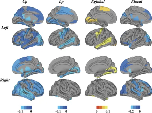
Looking at which brain’s regions show a significant variation in topological functional newtork parameters, all of the typical default mode network can be identified as shown in fig.(1.4).
This and many other studies relating to different types of disorders, show how investigating and modeling the default mode networks is of great impor-tance in classification and preventive diagnosis methods implementation.
Figure 1.4: Surface rendering of the distribution of altered nodes at a connec-tion density of 22%. Colored bars indicate differences in network properties between the NC and AD groups. Blue indicates regions showing an increase in the AD group but not the NCs. Yellow indicates regions showing a decrease in the AD group but not the NCs. In the AD group, the regions showing sig-nificant increases inCp, Lp andElocal are widely distributed across the brain, especially in default mode network regions such as the ACC, PCC, MPFC, HIP and IPL. Source: Xiaohu Zhao , Yong Liu et al. 2012 [6]
1.2
Investigating the Resting State
1.2.1
The fMRI Technique
The magnetic resonance imaging (MRI) is a non-invasive method largely used to obtain images of inner structures such as the human body. The method is based on the magnetic properties of materials composed of nuclei having a non-zero spin. Such nuclei, when placed in a magnetic field B0, arrange
themselves over energetic levels according to the Boltzmann distribution, with the total magnetization characterizing the order.
After introducing a perturbating pulse, which has to satisfy theresonance condition of the system, the magnetization tends to realign itself with B0
after a characteristic time, in which nuclei make transitions to set back the equilibrium. The MRI follows the evolution of the system during the return to the equilibrium, obtaining informations about a system’s properties and components via their characteristic time.
Let us consider an atomic nucleus with a non-zero total nuclear spin −→I ;
the relation between the magnetic momentµ and the spin is:
µ=γ}I (1.1)
where γ is the magnetogyric ratio, which is tied to each nuclear isotope.
Thus, the component along the z direction of the magnetic moment is:
µz =γ}m (1.2)
where m can take one of the 2I+ 1 values in the interval[−I, I].
For I = 1
2, an homogeneous applied external magnetic field B0 induces a
splitting of the nuclear spin energy level:
∆E =γ}B0 (1.3)
Replacing the Planck-Einstein relation ∆E = hν in the latter equation,
the Larmor resonance frequency is obtained:
ν0 =
γ
The corresponding pulsation ω0 is given by:
ω0 =γB0 (1.5)
The collective motion of a set of N nuclei can then be observed by means
of the total magnetization −M→=Nh−→µi.
The evolution in time of the magnetization of a set of nuclei placed a magnetic field B0 is:
d−M→ dt =γ
−→
M ×B0 (1.6)
The equation describes the precession of −→M around −B→0 at the angular
velocity ω0, when−M→ is not aligned with −B→0.
At the equilibrium, the total magnetization of a paramagnetic material placed in a magnetic field −B→0, shares the same direction of −B→0 as stated by
Curie’s law: −→ M0 =C −→ B0 T (1.7)
whereT is the absolute temperature andC is theCurie costant that tied
to material characteristics.
For the sake of simplicity −B→0 and −→M0 are considered aligned with the z
axis.
Applying a magnetic field −B→1 orthogonal to −B→0 with frequency ν0 causes
the magnetization vector to move away from the z axis; the angle between
the z axis and the new position of the magnetization vector depends on the
duration of the radio frequency (RF) field−B→1 applied, generated by a coil. At
the end of the pulse application, the spin precession on the transverse plane induces an oscillatory electromotive force in the coil by electromagnetic in-duction, thus originating a current in the probe. The detectable signal is called Free Induction Decay (FID), which has an oscillating trend with
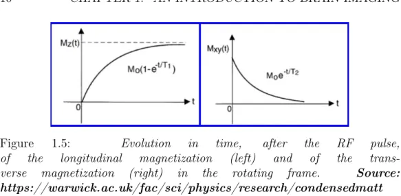
emitted by the set of nuclei getting back to equilibrium. After the RF pulse, the deacy of the NMR signal is analyzed in terms of two separate processes, the longitudinal one and the trasverse one, each with their own time con-stants. The underlying process that leads the longitudinal component of the magnetization (along z) to reach its equilibrium value M0, is the
redistri-bution of nuclear spin populations according to the Boltzman distriredistri-bution; such process takes place by energy exchanges between the nuclei and the surroundings.
The longitudinal component of the magnetization decreases in time, as defined by: dMz(t) dt =− (Mz(t)−M0) T1 (1.8) and thus: Mz(t) = Mz(0)e − t T1 +M 0(1−e − t T1) (1.9)
The underlying process that leads the trasverse component of the mag-netization to reach its equilibrium value, i.e. zero, is the decoherence of the transverse nuclear spin magnetization. Random fluctuations of the local magnetic field lead to random variations in the instantaneous NMR preces-sion frequency of different spins. As a result, the starting phase coherence of the nuclear spins is lost and the totalxy magnetization is null.
The transverse component of the magnetization decays to zero in time according to: dMxy(t) dt =− (Mxy(t) T2 (1.10) and thus: Mxy(t) =Mxy(0)e −t T2 (1.11)
1.2.2
The BOLD Signal
The Blood Oxygen Level Dependant signal is a measure of the amount of
Figure 1.5: Evolution in time, after the RF pulse, of the longitudinal magnetization (left) and of the trans-verse magnetization (right) in the rotating frame. Source: https://warwick.ac.uk/fac/sci/physics/research/condensedmatt
properly, the brain needs energy in the form ofAdenine-TriPhosphate (ATP),
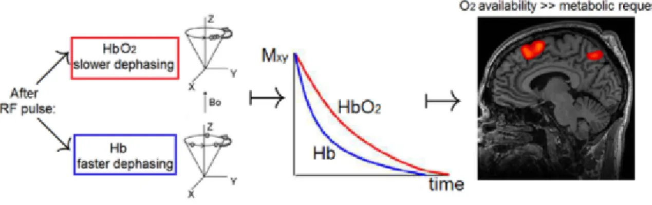
which is in turn produced through a chemical reactions involving glucose and oxygen. As neither glucose nor oxygen are stored in the brain by default, they need to be carried to the brain via circuclatory system. Oxygen is transported by haemoglobin, in a chemical form known as oxy-haemoglobin, in contrast to deoxy-haemoglobin, the form haemoglobin assumes when it releases the transported oxygen.
These two molecular forms differ by their magnetic properties: oxy-haemoglobin is paramagnetic, whereas deoxy-haemoglobin is diamagnetic (fig.(1.6)).
Figure 1.6: Deoxy-haemoglobin is trongly paramagnetic due to 4 un-paired electrons at each iron center. Source: mriquestion.com/bold-contrast.html
When energy is required in a particular area, or in other terms a partic-ular cerebral area is activated due to a given cognitive task, the amount of incoming oxygen (oxyhaemoglobin) is much higher than the oxygen being consumed to form ATP. As a result these areas show an increase in signal intensity. More precisely, since the deoxyhemoglobin is paramagnetic, it is able to reduce the NMR signal in T2 weighted images: indeed the rate of
loss of proton spin phase coherence, measured throughT2, can be modulated
by the presence of intravoxel deoxyhaemoglobin. On the contrary, being the oxyhemoglobin diamagnetic, it does not modify the NMR signal.
Thus, during the neural activation of a brain area, an higher incoming blood flux is observed with respect to the blood incoming during rest; in such area blood vessels expand and the transported oxygen rate is higher than oxygen consumed rate in burning glucose.
Therefore, although paradoxical, in the active brain region the concentra-tion of oxygenated blood increases, and the concentraconcentra-tion of deoxygenated blood decreases with respect to the neighbour inactive brain areas. Such process is shown in fig.(1.7).
Figure 1.7: BOLD signal formation process
It has to be pointed out, however, that the oxygen influx iunderlying the BOLD signal is not an immediate consequence of neural activity;they are rather parallel processes. In factGlutamate-generated Calcium influx releases
many vasodilators. Blood flow is related more to local field potentials than
individual neurons spiking [7]; it can therefore be statede that the signal is increased over an area larger than the one with specific neuronal activity.
Given the high number of processes underlying global blood flow changes, a model tying BOLD signals to neural activity is required for those fMRI aplications whose goal is to observe and characterize neural processes. The
link between the the BOLD signal and the effective neural signal lies in the
haemodynamic response function (HRF). Formally, the BOLD signal can be
interpreted as aconvolution between the actual neural signal and the HRF;
the system’s response to the stymulus is in ths way obtained.
If we take N(t)as the neural activity signa and h(t) as HDF we have:
B(t) = N(t)∗h(t) =
Z t
0
N(τ)h(t−τ)dτ (1.12)
In order for eq.(1.12) to be true, the assumption that the system’s response islinear and time invariant has to be made. We then define the neural signal
as:
N(t) =
Z ∞ t=0
δ(t−τ)nτdτ (1.13)
Given that the BOLD function is a function of neural activity B(t) =
f(N(t)), linearity implies that:
f( Z ∞ t=0 δ(t−τ)nτdτ) = Z ∞ t=0 f[δ(t−τ)]nτdτ (1.14)
thus proving eq.(1.7).
Although many evidences indicate that BOLD signal is non-linear, devia-tions from linearity are often small and linearity assumpdevia-tions are quite valid in many cases and apllications. As the HRF depends on the ways oxygen is consumed when energy is required by neurons, it is complex to model as a function. Even though eq.(1.7) holds true, most of the possible issues derive fromN(t)andh(t)being both unknown in a large number of problems. As a
result, the HRF is oftenestimated in order to be able to calculate the neural
signal. Many of the commonly used estimation methods rely upon recording the response to a given neural input, deconvolving eq.(1.7) while assuming a model for N(t), or trying to guess the function and smooth it with some
kind of parameter fitting.
Whichever the technique employed, one main feature of the HRF Must be taken into account for the consequences it induces on the BOLD signal
10 seconds) to reach its maximum value after neural activation. As a con-sequence, for short and close neural impulses, the BOLD response does not have the chance to decrease, because of the convolution with the HRF. It thus can be stated that BOLD always smooths the real underlying neural
signal.
1.2.3
Data Preprocessing
The aim of data preprocessing is to reduce the statistical noise, in order to better extract the true signal. This is most important for resting state analysis, given that there is no peak in the time series compared to the average value of the entire series. Looking at fig.(1.2) in example, we can see that, as a matter of facts,changes in BOLD signal rarely exceed the 1%.
A resume of the most common preprocessing practices for fMRI studies is done in the following section.
• Slice-timing correction: All fMRI data are collected inslices, which
in turn contain arrays of voxels.
The Repetition Time TR is the time which separates the onsets of
consecutive whole brain scans; thus is the time needed to collect data from all the brain voxels at a given point in time. This causes some problems to arise, i.e. not all the brain voxels in a given TR are acquired simultaneously: a TR time is needed to take all the slices between the first and the last. The bias is dependent on the order in which slices are taken. The most common approach to deal with such an issue is a form of temporal interpolation, which can be linear, spline, or sinc.
Linear interpolation is good when data do not vary much rapidly from one time acquisition to the other. This approach simply consists of estimating a continuous BOLD function from the discrete sampling; when using a linear function, a simple line is estimated between two points, and the value at the point of interest is taken.
• Head motion correction: It is probably the most important
prepro-cessing step.
During task studies, a movement of5mmcan increase activation values
by a factor of 5, and it can completely mix up signal from different
voxels in resting state studies. All the corrections are based on the assumption that during movements the brain does not change size or shape; as a result, the only changes are due to rigid body movement. As
a matter of fact, the movement can be characterised bysix parameters,
3 translational and 3 rotational, as described by classical mechanics. Voxels are defined by their position within the scanner,rather than by position within the subject’s brain. To correct for this a rigid body registration is performed.
• Normalization: each individual presents morphologically different
brains, with different global size and different local regions sizes too. This leads to many problems while studying if a signal observed in one region is observed in the same region in another patient. Moreover, when performing group analyses, brains have to be overlapped, in order to increase the signal to noise ratio and the statistical significance of the analysis. However, if we overlap two significally different regions, the signal is quite likely to average out. Therefore, warping one subject’s structural image to astandard brain atlas is a required step. The most
common reference system is the MNI space, developed by the Montreal Neurological Institute [8].
• Coregistration: functional data have to be mapped onto structural
data in order to as- sess the exact region the signal is coming from. These is not straightforward due to the two images being taken with different spatial resolutions. Given that functional images have to be taken within a few seconds, as a consequence of a speed-accuracy trade-off, they often have poor spatial resolution. Structural images, on the other hand, can take up to 10 minutes in order to be acquired if a precise mapping of every region is to be obtained. This results in different voxel sizes: a typical fMRI voxel is(3×3×3.5)mm, whereas sMRI can have
voxels with sizes down to (0.86.86×0.89)mm. After coregistration,
however, structural resolution can be employed to improve functional resolution. Early methods aimed at identifying key landmarks in the two different images and then trying to align them, but given the scarce automation reliabiity of this process most methods now relies upon the minimisation of mutual information between histograms of the images. • Data smoothing: intensity values from individual voxel have an
em-bedded component of noise.
In order to reduce this noise spatial smoothing is needed; basically the intensity value of a voxel is replaced with a weighted average of the values of neighbouring voxels, through the convolution between the voxels and a function representing the neighbourhood known askernel.
Other than increasing SNR, this process is useful since, as explained by the central limit theorem, it allows the distribution of intensities to
become normal thus helping the multiple comparison analysis in task studies.
1.2.4
The Functional Connectivity Matrix
One of the most common approaches in resting state studies gravitates around the notion of Functional Connectivity. Functional Connectivity is defined as the statistical association or dependency among two or more anatomically distinct time-series [9].
In FC analyses, there is no inference about coupling between regions; that is it does not tellhow regions are coupled. In fact, it only tests some form of
correlation against the null hypothesis. FC is however useful todiscover pat-terns (which regions are coupled), and compare patterns, especially between
groups. In practice FC can be represented by a matrix whose entry aij is a
correlation between the intrinsic activity of neural sourceiand neural source j.
Common examples of correlations measures computed on time-series data types are the cross-correlation and cross-coherence [9]. Cross correlation
between regions 1 and 2 with a time delay t is given by: R(t) = p cov(s1, s2 +t)
var(s1) +var(s2 +t) (1.15)
Cross-coherence can be defined as equivalent to cross-correlation but in the frequency domain. It is defined as follows:
Coh(f) =| (Ψ1,2)
2
((ψs1(f))ψs2(f))|
(1.16) Where Ψ1,2 is the cross-spectral density; ψs1,2 are the spectral density of
regions 1 and 2. Coh(f) varies between 0 and 1 and is defined for different
The Wishart Distribution
2.1
Definition
The wishart distribution Wp(n,Σ) is a probability distribution of random
nonnegative-definitep×p matrices that is used to model random covariance
matrices.
The parameternis the number of degrees of freedom, andΣis a
nonnegative-definite symmetric p×pmatrix, called the scale matrix.
Def. Let X1...Xn be Np(0,Σ) distribuited vectors, forming a data matrix
p×n, X = [X1...Xn]. The distribution of a p×p, M = XX0 = Σni=1XiXi0 random matrix is a Wishart distribution. [10]
We have then by definition:
M ∼Wp(n,Σ)∼Σni=1XiXi0 Xi ∼Np(0,Σ) (2.1)
so that M ∼Wp(n,Σ)is the distribution of a sum ofn rank-one matrices
defined by independent normal Xi ∈Rp with E(X) = 0 and Cov(X) = Σ.
In particular, it holds for the present case:
E(M) = nE(XiXi0) =nCov(Xi) =nΣ (2.2)
2.2
PDF Computation for Invertible
Σ
In general, anyX ∼N(µ,Σ) can be represented as
X =µ+AZ, Z ∼N(0, Ip) (2.3)
so that
Σ =Cov(X) =ACov(Z)A0 =AA0 (2.4)
The easiest way to find A in terms of Σ is the LU-decomposition, which
finds a unique lower diagonal matrix A with Aii>0 such thatAA0 = Σ.
Then by 2.1 and 2.4, with µ= 0 we have:
Wp(n,Σ)∼ n X i=1 (AZi)(AZi)0 ∼A( n X i=1 ZiZi0)A 0 ∼AWp(n)A0 (2.5) whereZi ∼N(0, Ip)and Wp(n) =Wp(Ip, n).
Assuming thatn ≥pand Σis invertible, the density of the randomp×p
matrix M in 2.1 can be written 1 :
f(M, n,Σ) = 1 2np2 Γp(n 2)kΣk n 2 k Mkn−2p−1exp[−1 2trace(Σ −1M)] (2.6)
so that f(M, n,Σ) = 0 unless M issymmetric and positive-definite. [11]
Note that in 2.6 we define Γp(α) as the generalized gamma function: Γp(α) =π p(p−1) 4 p Y i=1 Γ(2α+ 1−i 2 ) (2.7)
2.2.1
Visualizing the Wishart Distribution
The Wishart distribution is a generalization to multiple dimensions of the
chi-squared distribution, or in the case of non-integer degrees of freedom, of
Figure 2.1: Monodimensional Wishart Distribution and χ2(n) distribution comparison
We show in fig.2.1 that for a 1-dimensional and equal to 1Σscale matrix,
the Wishart distribution W1(n,1)is equivalent to the χ2(n) distribution.
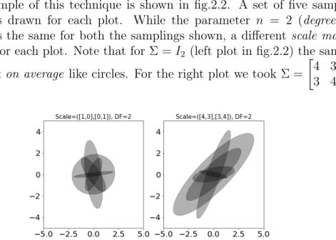
Save for this simple case, being the Wishart a distribution over matrices, it is a generally hard task to visualize it as a density function. We can however sample from it and use the eigenvectors and eigenvalues of the resulting sampled matrix to define an ellipse.
An example of this technique is shown in fig.2.2. A set of five sampled matrices is drawn for each plot. While the parameter n = 2 (degrees of freedom) is the same for both the samplings shown, a different scale matrix Σis used for each plot. Note that for Σ = I2 (left plot in fig.2.2) the sample
would look on average like circles. For the right plot we took Σ =
4 3 3 4
Figure 2.2: Plot of eigenvalue and eigenvectors defined ellipses, drawn from different scale matrix defined by a Wishart-sampled distribution.
1Note:
2.3
The Wishart Distribution in Bayesian
Con-jugate Prior Analysis
An important use of the Wishart distribution is as a conjugate prior for
multivariate normal sampling. We now recall some basics concepts about
Bayesian inference and prediction in order to show the application of the Wishart in those fields.
2.3.1
Bayesian Inference and Priors Distributions
The distinctive feature of the Bayesian approach underlies in its way of defin-ing probability.
Probability is treated as belief and not as frequency, thus introducing a
fundamental difference between the Bayesian and the frequentist approach
and shifting the goal toward the analysis and statement of abelief [12].
We can sum up the process of Bayesian inference as follows:
• A probability density calledprior distributionπ(θ)is chosen, expressing
the beliefs about a parameter θ before any data are seen.
• A statistical model p(x | θ) is chosen, which must reflect the beliefs
about x given θ.
• After observing the data Dn = [X1...Xn], the beliefs is updated and
the posterior distribution p(θ|Dn) is computed.
By Bayes’ theorem the posterior distribution can be written as
p(θ |X1...Xn) = p(X1...Xn|θ)π(θ) p(X1...Xn) = Ln(θ)π(θ) cn ∝ Ln(θ)π(θ) (2.8)
whereLn(θ) = Qni=1p(Xi |θ)is the likelihood function and the normaliz-ing constant cn is defined as follows:
cn=p(X1...Xn) = Z
p(X1...Xn|θ)π(θ)dθ = Z
Ln(θ)π(θ)dθ (2.9)
We now define the general properties of a conjugate prior. If, for a given
problem, the posterior distribution p(θ |X1...Xn) and the prior π(θ) belong
to the same family of distribution, they’re called conjugated distributions
and the prior is said to be a conjugate prior for the given likelihood function
Ln = p(X1...Xn | θ). Note that in order for this to be a meaningful notion,
the family of distribution should be sufficiently restricted, and is typically taken to be a specific parametric family. Complete characterization of the conjugate priors exists only for general exponential family models [12].
Considering the general problem of inferring a distribution for a parameter
θ given some observations Dn = [X1...Xn] and referring to theorem 2.8,
by which we let the likelihood function be considered fixed as it is usually well-determined from a statement of the data-generating process, it is clear that different choices of the prior distribution π(θ) may make the integral
in 2.9 more or less difficult to compute. The product Ln(θ)π(θ) will also be
influenced, gaining the possibility to take one algebraic form or another. If for certain choices of the prior the posterior has the same algebraic form as the prior, those choices are said to yield a conjugate prior. It is then
possible to state that a conjugate prior is an algebraic convenience giving a closed-under-sampling-form expression for the posterior.
A classical example concerns the Gaussian Distribution: the Gaussian family is conjugate to itself (or self-conjugate) with respect to a Gaussian likelihood function: if the likelihood function is Gaussian, choosing a Gaus-sian prior over the mean will ensure that the posterior distribution is also Gaussian [13].
2.3.2
The Wishart Conjugate Prior
We now show how the Wishart Distribution is correlated to theInverse Gamma Distribution in a multidimensional setting, by considering a Gaussian model
with known mean µ, so that the free parameter is the variance σ2, as in
[12]. By doing so, we justify the use of the Wishart distribution in modelling estimated distribution under the assumption of Multivariate Gaussian dis-tributed data scenarios. This kind of assumption is indeed generally good for a wide range of problems. Furthemore, the use of the average of one class’s covariance matrix to compute the scale matrix for the class estimated dis-tribution will be proved to be a good approximation of a complete Bayesian model.
The likelihood function is defined as follows: p(X1...Xn |σ2)∝(σ2)− n 2exp(− 1 2σ2n(X−µ 2)), (X−µ2) = 1 n n X i=1 (Xi−µ)2 (2.10)
The conjugate prior is an inverse Gamma distribution. Recall that θ has
an inverse Gamma distribution with parameters(α, β)when 1
θ ∼Gamma(α, β).
The density is then bound to take the form
πα,β(θ)∝θ−(α+1)e−
β
θ (2.11)
Using this prior, the posterior distribution of σ2 is given by p(σ2 |X1...Xn)∼InvGamma(α+ n 2, β+ n 2(X−µ 2)) (2.12)
An alternative way of parameterization of the prior is given by theInverse Scaled χ2 Distribution, whose density is defined as
πν0,σ02 ∝θ −(1+n0 2 )exp(−ν0σ 2 0 2θ ) (2.13)
Under this kind of parameterization of the prior, the posterior takes the form p(σ2 |X1...Xn)∼ScaledInvχ2(ν0+n, ν0σ02 ν0+n + n(X−µ 2) ν0+n ) (2.14)
In the multidimensional setting, the inverse Wishart takes the place of the inverse Gamma.
It has already been stated that the Wishart distribution is a distribution over symmetric positive semi-definite d×d matrices W. A more compact
form of the density is given by πν0,S0(W)∝|W | (ν0−d−1) 2 exp(−1 2trace(S −1 0 W)), |W |=det(W) (2.15)
where the parameters are the degrees of freedom ν0 and the
positive-definitescale matrix S0.
If W−1 ∼ W ishart(ν
0, S0) we can then state that W has an Inverse
Wishart Distribution, whose density has the form
πν0,S0(W)∝|W | −(ν0+d+1) 2 exp(−1 2trace(S0W −1)), |W |=det(W) (2.16) LetX1...XnbeN(0,Σ)distributed observed data. Then an inverse Wishart
prior multiplying the likelihood p(X1...Xn |Σ)yields
p(X1...Xn|Σ)πν0,S0(Σ) ∝ |Σ|−n2 exp(−n 2trace(SΣ −1) |Σ|−(ν0+2d+1) exp(−1 2trace(S0Σ −1)) =|Σ|−(ν0+d2+n+1) exp(−1 2trace((nS+S0)Σ −1)) (2.17)
where S is the empirical covariance S = 1
n Pn
i=1XiX
T i .
Thus, a posterior with the form
p(Σ|X1...Xn)∼InvW ishart(ν0+n, nS+S0) (2.18)
is obtained.
Analogally, it can be stated that for the inverse covariance (precision)
The WISDoM Multiple Order
Classification
In this section, the classification method implemented and used on the ADNI2 database is described, both in an analytical and technical way.
The Wishart Distributed Matrices Multiple Order Classification is a method that allows both classification andfeature selectionfor any classification
prob-lem whose eprob-lements can be tied to a symmetric positive-definite matrix
rep-resentation (i.e. covariance and correlation matrices). The measure used to
train the classifier is defined as well as thefeature transformation undergone
by the each of the subject analyzed. The general pipeline and the valida-tion pipeline are then discussed while also introducing an example of possible parallelization for performance enhancing.
3.1
Wishart Sampling
Considering what has been said in the last section, using the Wishart distri-bution to model and sample the elements of a wide range of problems follows naturally.
As a matter of fact, every calssification problem whose elements take the form of symmetric positive-definite matrices can be approached with the
method we are about to discuss. The main idea for the WISDoM Classifier
is to use the free parameters of the Wishart distribution (the scale matrix
S0 and the number n of the degree of freedom, as shown in 2.6) to compute
an estimation of the distribution for a certain class of elements, and then 25
assign a single element to a given class by computing some sort of "distance" between the element being analyzed and the classes.
Furhermore, if we assume that the matrices are somehow representative of the features of the system studied (i.e. covariance matrices might be taken
into account), a score can be assigned to each feature by estimating the weight of said feature in terms of Log Likelihood Ratio. In other words, a
score can be assigned to each feature by analyzing the variation in terms of LogLikelihood caused by the deletion of it. If the deletion of a feature
causes significant increase (or decrease) in theLogLikelihood computed with
respect to the estimated distributions for the classes, it can be stated that
said feature is highly representative of the system analyzed.
It is now clear that the simplest usable objects to estimate the distribution for a class and to represent its elements is the covariance matrix. Further
proofs for this statement will be given later on. Thus, the aim of the WISDoM classifier is not only to assign a given element to the optimal class, but also to identify the features with the highest "weights" in the decision process.
3.1.1
Computing the Estimated Distribution
Let us briefly recall the parametrization of the Wishart Distribution in order to clearly define the application conditions for classification problems.
Let X1...Xn be independent Np(0,Σ)distributed vectors, forming a data
matrix p×n, X = [X1...Xn]. The distribution of a p×p, M = XX0 = Σn
i=1XiXi0random matrix is a Wishart distribution with parametersWp(n, S0).
In the previous chapter (2.6) it has been proved that for normal distributed data, for S0 = Σ, a distribution of random covariance matrices is obtained.
In a similar fashion, if a good choice for the scale matrix S0 is made for a
given class, a representative distribution for the class can be estimated and samples can be drawn from it.
Covariance matrices are a good choice, although not limiting as long as the
matrices are symmetric and positive-definite, both for the way they represent a system and for the property that the mean of a set of covariance matrices is a covariance matrix.
If each element of a given classC is represented by a covariance matrix Σ
by choosing S0 = ˆΣC = 1 N N X i=1 Σi (3.1)
The other necessary parameter for the estimation is thedegrees of freedom n.
Assume that an Xi = (x1, ..., xp) vector of pfeatures is associated to each
element i of a given class, while having n observation of said vector. The
covariance matrix Σi computed over the n observations will represent the
"interactions" between the features of element i. The degrees of freedom n of the Wishart distribution are then given by the number of times Xi is
observed.
Let us introduce an example tied tofunctional MR brain imaging in order
to further clarify the concepts being introduced.
An image of patienti’s brain is acquired; as usual these images are divided
in a certain number p of zones (voxel, pixel etc.), each zone being sampled n times over a given time interval in order to observe a certain type of brain
activity and functionality. It is now clear that the features contained in vector Xi = (x1, .., xp) associated to patient i are indeed the zones chosen
to divide i’s brain image, each zone having been sampled n times during
an acquisition interval. The correlation p×p matrix Σi computed for i’s
observation is then representative of the functional correlation between the
p zones of i’s brain. Repeating this procedure forN patients belonging to a
known class C (i.e. a diagnostic group) and computing the ΣˆC scale matrix
for the class as stated before, will allow us to estimate a wishart distribution for that class correlation matrices and draw samples from it.
The module used for Wishart generation and sampling by the WISDoM calssifier is the SciPy.Stats.Wishart module of theSciPy Python3.6 library.
Further details on the generation and sampling algorithm used by the module can be found in [14].
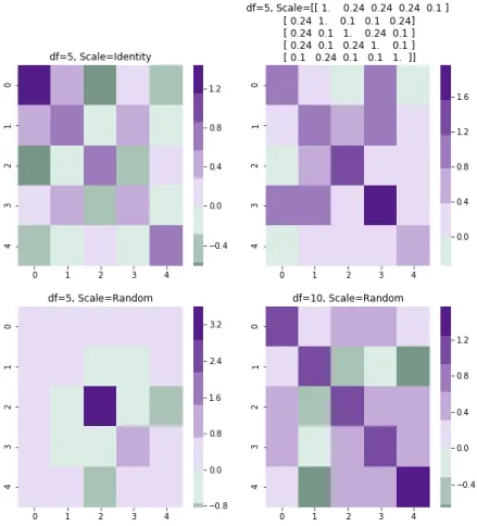
Some samples drawn from Wishart distributions computed with different
Figure 3.1: Various sampling from different wishart distribution. A diverging heatmap has been chosen to visualize the values of each sample’s elements.
3.2
Log-Likelihood Ratio Measure
After the definition of the role of the Wishart distribution in symmetric posi-tive definite matrices’ modeling, it is necessary to define some sort of distance between the estimated distribution for a classC and its hypotetical elements.
As stated before, this will be done in terms of both entire matrices and sin-gle features, in order to achieve optimal classification and exract information
3.2.1
Complete Matrix Measure
The scoring system used by the WISDoM Classifier relies on thelogpdf
func-tion from the SciPy.Stats.Wishart module in order to compute the
LogLike-lihood of a matrixΣi with respect to the Wishart distribution estimated for
a class C, using ΣˆC as the scale marix. If a problem concering two given
classes CA and CB is taken into account, the score assigned to each Σi upon
which the classification decision is based, can be defined as follows:
scorei =logPW(Σi |n,ΣˆA)−logPW(Σi |n,ΣˆB) (3.2)
Where ΣˆA,B are the scale matrix computed for the classes A, B and
logPW(Σi | n,ΣˆA,B) can be seen as the logarithm of the probability of Σi
belonging to the Wishart distribution estimated for one of the two classes
A, B.
3.2.2
Single Feature Measure and Multiple Order
Re-duction
The aim of the WISDoM classifier is to further increase the informations obtained about the system’s features during the classification.
To do this it is then necessary to introduce some matemathical properties of the symmetric positive deifnite matrices, upon which the method relies. It will be shown that it is indeed possible to access different orders of infor-mation by scaling a matrix A to its principal submatrices.
Def. Let A be an n ×n matrix. A k × k submatrix of A formed by deletingn−k rows ofA, and the same n−k columns of A, is called principal submatrix of A. The determinant of a principal submatrix of A is called a principal minor of A.
Note that the definition does not specify which n−k rows and columns
to delete, only that their indices must be the same. Let us introduce a 3×3example.
For a general matrix A3×3 A= a11 a12 a13 a21 a22 a23 a31 a32 a33 (3.3)
there are three first order principal minors:
• |a11| formed by deleting the last two rows and columns
• |a22| formed by deleting the first and third rows and columns
• |a33| formed by deleting the first two rows and columns
There are three second order principal minors:
• |
a11 a12
a21 a22
| formed by deleting column 3 and row 3
• |
a11 a13
a31 a33
| formed by deleting column 2 and row 2
• |
a22 a23
a32 a33
| formed by deleting column 1 and row 1
There’s one third order principal minor, namely|A|.
For the sake of completion, we also recall the following definition.
Def. Let A by an n×n matrix. The kth order principal sub-matrix of A
obtained by deleting the last n−k rows and columns of A is called the kth
order leading principal submatrix of A, and its determinant is called the
kth order leading principal minor of A.
An imporant property for the principal submatrices of a symmetric posi-tive definite matrix is that any (n−k)×(n−k) partition is also symmetric and positive definite.
It is now clear that such properties can be used to reduce both a class scale matrix ΣˆC and any Σi matrix, in order to study its deviation from a
class’s estimated Wishart distribution derived from the deletion of one of its components (the features conatined in vector Xi = (x1, ..., xp) from which
Iterating this process over all the features, or in other terms analyzing all of the (p−1)×(p−1)principal submatrices of Σi and ΣˆC, will allow us to
assign a score to each feature, representing its weight in the decision for Σi
to be assigned to one class or another.
Note that for such an order of principal submatrices, the process will reduce the Σi,p×p matrix to a score vector of length p for each element i
undergoing the classification.
Let us now introduce the following notation in order to define the score assigned for each of the xp features of the vector Xi = (x1..., xp).
LetΣj be a principal submatrix of order(p−1), of the matrixΣcomputed
on the observation of Xi = (x1, ..., xp) for subject i, obtained by the deletion of the jth row and the jth column, with 1≤j ≤p.
Let ΣˆCj be a principal submatrix of order (p − 1), of the matrix ΣˆC
computed for the class C obtained by the deletion of thejth row and the jth column, with 1≤j ≤p.
The score assigned to each feature of Xi = (x1, ..., xp) is then given by
eq.(3.4).
Scorej(C) = ∆logPW j(C) =logPW(Σ, n|ΣˆC, n)−logPW(Σj, n |ΣˆCj, n)
(3.4)
In other terms, each partition Σj represents the matrix Σ without the
elements tied to featurexj (the elements in row j and column j of Σ).
Com-puting the variation in terms of log-likehood between the estimated wishart distribution for the class and the estimated wishart distribution for the class without component j, allows us to gain informations about which feature
weighs more on both subject i’s cassification and the general system
struc-ture.
Note that this kind of scoring is class-dependent. Computing this score
vector with respect to all the classesC1..Cnof a given problem and performing
some sort of score ratio will allow the subject i, after a suitable training, to
be assigned to the most likely of the classes while retaining informations on which features are the most determinant, decision wise.
Let us introduce a 2-classes example in order to show how this kind of
result might be obtained.
Let C1 and C2 be the two classes of a given problem.
Let a set of N matrices Σi be a set of correlation matrices computed for
N subjects i whose class is known.
LetΣˆC1 and ΣˆC2 be the scale matrices computed as seen in eq.(3.1), used
to estimate the Whishart distribution for each one of the two classesC1 and
C2, and ΣˆC1j and ΣˆC2j their (p−1)order partitions, as in eq.(3.4).
If from each matrix Σi the score vector is computed as in eq.(3.4) with
respect to each one of the two classesC1, C2, aninter-class log-likelihood ratio
vector can be obtained by assigning to each feature a score defined as follows:
Ratioj = ∆logPW j(C1)−∆logPW j(C2) (3.5)
Training a classificator on a set of N subjects whose classes are known,
after each matrix Σi (and as a consequence each feature vector Xi) has
un-dergone the transformations defined in eq.(3.4) and (3.5), yields a significant improvement in performance for certain classes of problems, as it will be shown later.
A new subject will be, as a matter of fact, classified according to its
transformed ratio vector given by eq.(3.5), thus simultanesously retaining
information about its class’s most significant features: the score assigned to each feature is a measure of how much the deletion of said feature weighs, in terms of log-likelihood variation, on the decision to assign each matrix Σi to one class or another.
The entire process can be seen as a feature transformation, which leads to
afeature selection, whose effect is, for certain types of problems, to enhance
the classification performance.
3.2.3
Generalizing to
(
p
−
n
)
Order Transformations
As seen in the last section, transforming all the (p−1)×(p−1) principal
submatrices of Σi by eq.(3.4), yields a vector of score of length p for each
Anyway, for any n < p, a number of principal submatrices of Σi can be
obtained. These kind of submatrices can be used to gain informations about the weight ofnsimoultaneously deleted features on the system structure and
classification. Let us introduce an example for(p−2)order submatrices.
Let Σjk be a principal submatrix of order (p−2), of the matrix Σi
com-puted on the observation of Xi = (x1, ..., xp) for subject i, obtained by the deletion of the jth row and the jth column and the kth row and the kth column
, with 1≤j, k ≤p.
Let ΣˆCjk be a principal submatrix of order (p−2), of the matrix ΣˆCjk
computed for the class C obtained by the deletion of thejth row and the jth column and the kth row and the kth column , with 1≤j, k ≤p.
Then, eq.(3.4) becomes:
Scorejk(C) = ∆logPW jk(C) =logPW(Σ, n|ΣˆC, n)−logPW(Σjk, n |ΣˆCjk, n)
(3.6)
in this case, a score is assigned to each coupling of the features j, k, and
transformation (3.6) will yield not a vector, but ap×pmatrix with diagonal
elements equals to the scores obtained by (3.4), being the iteration withj =k
the coupling the jth feature with itself. Non-diagonal elements represent the
score of the coupling of featurej with feature k.
A notable characteristic of (p−2) order transformations for correaltion
matrices, is that the informative content after such an order of transformation is comparable to that of the original correlation matrix. It can thus be stated that the (p−2) order transformed correlation matrix seems to be equivalent to the original correlation matrix under an affine transformation.
3.3
Pipeline
In this section we discuss each step of the feature transformation and classi-fication process.
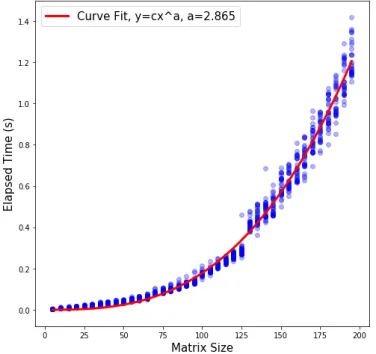
Given the recursive nature of the method just described, a crucial issue concerning computational time is the strong dependence between it and the analyzed matrix size. A rough visualization of the entity of such a dependence can be found in fig.(3.2)
Figure 3.2: Matrix Size dependence for (p−1) order transformations. The jump between the 125-150 size range maybe due to upcoming cache storing processes.
Iterating the (p− 1) order transformation described in eq.(3.4) over a
large N of observations of size p×p of a given database, while introducing
some kind of cross-validation routine may lead to abysmal computational
time-wise performances.
A possible solution to this problem is to introduce a high level of automa-tization for each step, followed by the indroduction of a highly parallelizable overall structure of the pipeline.
3.3.1
The Snakemake Environment
The main tool used to achieve such results is the Snakemake Workflow Management System, described in [15], a Python-based interface created to
To briefly some up the the advantages of using such tools and structures, the Snakemake Workflow can be described as rules that denote how to
cre-ate output files from input files. The workflow is implied by dependencies between the rules that arise from one rule needing an output file of another as an input file [15].
A rule definition specifies :
• a name, used by the main rule instance rule all and main execution
environment for identification
• any number of input and output files; tipically one rule’s output is
an-other rule input, linking the rules alla the way up to main rule instance. • either a shell command or Python code; containing the creation of the
output from the input
Input and output files may contain multiple named wildcards, whose values
are inferred automatically from the files desired by the user.
To further clarify the role of the wildcards, let us introduce a brief exam-ple. Let’s say that our aim is to train a classifier over two classes of elements
C1, C2. The training part of the database is then divided in two files, each
one containing the name of its elements’ class in the filename. Setting a rule to load these files while expecting a wildcard tied to the class name in the filename, will allow the entire set of rules of the pipeline to be executed auto-matically for classC1 and classC2. Considering this example, the real power
of the parallelization capabilities offered by the Snakemake environment are quite clear.
With a simple syntax, looking at the example just proposed, each one of two cores of a server where our hypothetical pipeline is running can be set
to work indipendently on each subset of data belonging to class C1 or class
C2. Building a pipeline whose rules are easily iterable over a set of different
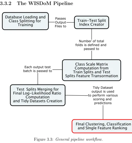
3.3.2
The WISDoM Pipeline
Figure 3.3: General pipeline workflow.
In figure (3.3) the main steps required by the WISDoM Multiple Order Classification are reported.
We will now go through each step in detail in order to show howtrain and test splitting are interpreted for the WISDoM pipeline.
• Database loading and class splitting
rules: case_wrap, seqs_store ; in this section of the pipeline, data are
loaded and divided into the classes defined by the wildcards and main rule instance’s inputs. An info sheet containing the classification labels for each observation is needed as aninput for this step.
In order to achieve fast reading/writing perfomances for big data, the matrices are stored as the sequence of elements belonging to the upper
triangle for each matrix (in.hdf format). Being symmetric, the entire
matrix can be easily reconstructed when needed. At this step, the files containing observations for each class are created.
• Train-Test split index creator
rules: split_gen, tt_gen; in this section of the pipeline, each file
con-taining one class’s observations is divided into train-test batches. The total number of train-test folds is defined by wildcards and main rule instance’s inputs.
First, each dataset is divided into sections, then each section is further splitted intoa number of user-specified train-test folds.
• Class Scale Matrix computation and feature transformation rules: map_gen; this is the core section of the pipeline, where the
features are transformed according to eq.(3.4).
Train-test split files for each class are passed as inputs; the train sets of each batch are used to compute the scale matrix ΣˆC as in eq.(3.1).
The estimated Wishart for the class is then computed and the features of each test-set element are transformed.
In order to compute the Ratio described in eq.(3.5), the above process is repeated for each class with respect to each other. A map containing each transformed feature in term of quantiles is also created.
• Test splits merging and tidy datasets creation
rules: t_join, q_join; in the final step of the pipeline, all of the
trans-formed feature test batches are merged into tidy datasets. This type of data sturcture will allow an easy computation of the ratio in eq.(3.5) for each feature; furhtemore, once such dataset is obtained, evertything needed for the transformed observations to undergo any classification pipeline and/or model selection is ready.
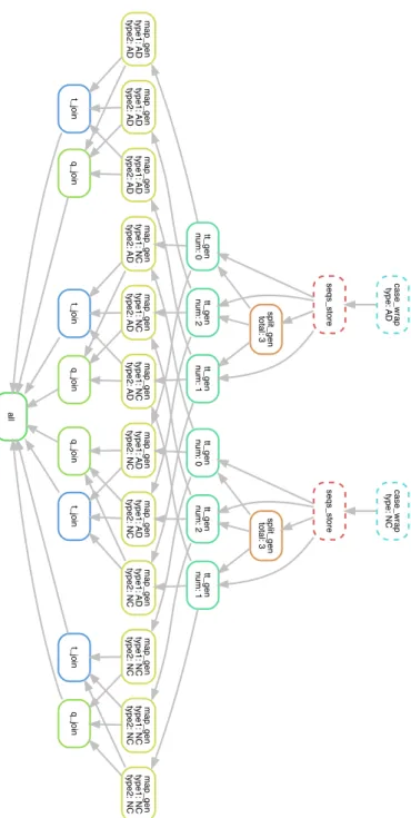
A graphic representation of the plan of rules execution can be obtained by using a directed acyclic graph (DAG), as shown in figure (3.4).
q_join all sp lit_ g e n total: 3 tt_gen n u m: 2 tt_gen n u m: 1 tt_gen n u m: 0 se q s_ st o re tt_gen n u m: 2 tt_gen n u m: 1 tt_gen n u m: 0 sp lit_ g e n total: 3 ma p _ g e n typ e 1 : AD typ e 2 : AD q_join t_join ma p _ g e n typ e 1 : AD typ e 2 : N C ma p _ g e n typ e 1 : N C typ e 2 : AD q_join ma p _ g e n typ e 1 : N C typ e 2 : N C t_join ma p _ g e n typ e 1 : N C typ e 2 : AD t_join t_join ma p _ g e n typ e 1 : N C typ e 2 : N C ma p _ g e n typ e 1 : AD typ e 2 : N C q_join ma p _ g e n typ e 1 : AD typ e 2 : AD ma p _ g e n typ e 1 : N C typ e 2 : AD ma p _ g e n typ e 1 : AD typ e 2 : AD ma p _ g e n typ e 1 : AD typ e 2 : N C ca se _ w ra p typ e : AD ma p _ g e n typ e 1 : N C typ e 2 : N C ca se _ w ra p typ e : N C se q s_ st o re
Figure 3.4: Directed Acyclic Graph representation of the WISDoM pipeline for the observations of ADNI database. Here we have 2 type of subject, labeled AD and NC, undergoing a 3 fold train-test split. This split has been chosen for visualization purposes; for the real analysis a 10-folds split has been used.
3.3.3
Classification Methods
The last steps of the pipeline are tied to clustering, classification and cross-validation on the dity dataset returned by the Snakemake section of the pipeline. We now present a brief excursus on the methods used on the ADNI2 database.
Note that once the tidy dataset [21] is obtained, a wide range of methods might be implemented in order to achieve clustering, classification, cross-validation and feature selection. The methods we used are thus just a narrow selection of all the possibilities.
Hierachical Clustering
In order to assess informations about classification performance and to find those feature whose weights are the most significant in assigning one element to a class or another, a hierchical clustermap might be used as a fast and
informative visualization. The tool chosen is the clustermap function of the Seaborn python 3.6 module, as described in:
seaborn.pydata.org/generated/seaborn.clustermap.html.
As in [20], hierarchical clustering’s performances are metric and linkage functions dependent.
For the ADNI2 database clustering, metric used is aL1City Block, defined
as
k X
j=1
|aj −bj | (3.7)
between two k dimensional pointsa, b.
In this way, the effect of a large difference in a single dimension is damp-ened (since the distances are not squared) [19]. As far as linkage functions are concerned, we used a Nearest Point Algorithm.
Suppose there are |u|original observations (u[0], ..., u[|u| −1]) in cluster
u and |v| original objects (v[0], . . . , v[|v| − 1]) in cluster v. Let v be any
remaining cluster in the forest that is not u.
The Nearest Point Algorithm assigns:
for all points i in cluster u and j in cluster v.
Other possible linkage alghorithm are [20]:
• Farthest Point Algorithm or Voor Hees Algorithm, assigns:
d(u, v) = max(dist(u[i], v[j])) (3.9)
for all points iin cluster uand j in cluster v.
• UPGMA algorithm, assigns:
d(u, v) = X ij
d(u[i], v[j])
(|u| ∗ |v|) (3.10)
for all points i, j where |u|,|v| are the cardinalities of clusters u, v
re-spectively.
Further weighted methods are described in [20].
Support Vector Machine Classification
Another one of the methods used for classification and cross-validation is a classic Support Vector Machine. The tool used is from the SKLearn Python 3.6 module. More details can be found at:
scikit-learn.org/stable/modules/generated/sklearn.svm.SVC.html
In general, a support vector machine can be seen as a generalization of linear decision boundaries for classification. In other terms, is a method to assess optimal separating hyperplanes for non completely separable classes
problems [22]. This is done by producingnonlinear boundaries by
construct-ing a linear boundary in a large, transformed version of the feature space. A comparison of how a support vector classifier operates to solve non-separable problems is reported in fig.(3.5)
Figure 3.5: Support vector classifiers. The left panel shows the separable case. The decision boundary is the solid line, while broken lines bound the shaded maximal margin of width 2M = 2
||β||. The right panel shows the
nonseparable (overlap) case. The points labeled ξj∗ are on the wrong side of their margin by an amount ξ∗j =M ξj; points on the correct side have ξj∗ = 0. The margin is maximized subject to a total budget P
ξi ≤ C. Hence P
ξj∗
is the total distance of points on the wrong side of their margin. Source: Trevor Hastie, Robert Tibshirani, Jerome Friedman [22].
Logistic Regression
A method used to asses informative content of single features is the Logistic Regression Once again, a SKlearn Logistic Regression classifier is used.
De-tails can be found at:
scikit-learn.org/stable/modules/generated/sklearn.linear/.
Logistic regression, is a regression model whose dependent variable is cat-egorical. It can be stated that logistic regression is used to predict the risk
of observing a given binary outcome; for example, patients survive or die, have heart disease or not, a condition is present or absent while taking into account observed characteristics of the patient. In general, the logistic re-gression model arises from the desire to model the posterior probabilities of the K classes via linear functions in x, while at the same time ensuring that
they sum to one and remain in [0,1]. When K = 2, this model is
biostatistical applications where binary responses (two classes) occur quite frequently [22].
The model has the form:
logp(G= (1, ..., K−1)|X =x)
p(G=k|X =x) =β(1,...,K−1)0+β T
(1,...,K−1)x (3.11)
Logistic regression models are usually fit by maximum likelihood, using the conditional likelihood of Ggiven X. Since p(G|X), G= (1..., K −1, K)
completely specifies the conditional distribution, the multinomial
distribu-tion is appropriate.
The log-likelihood for N observations is: l(θ) = N X i=1 logpgi(xi, θi) (3.12) where pk(xi, θ) =p(G=k|X =xi;θ). ROC AUC Score
The score used to asses informative content and classification capabilities for each feature’s logistic regression is theReceiver Operating Characteristic Area Under the Curve score. To grasp the meaning of theReceiving Operating Characteristic score, we can think as follows.
A ROC curve is created by plotting the true positive rate (TPR) against the false positive rate (FPR) of a classifier at various threshold settings. It is thus a plot of thesensitivity (or probability of detection) as a function of the fall-out (orprobability of false alarm). Examples of ROC curves are reported
in fig.(3.6).
If theArea Under the Curveis computed when using normalized units, we
obtain a value tied to the informative power of a classifier, with a completely uninformative classifier (i.e a classifier based on completely random choices) yielding a value of 0.5 [23].
Figure 3.6: Sample ROC curves. A completely ran-dom classifier will be located at point (0.5,0.5) while a perfect classification would be located at (0,1). Credits:
![Figure 1.2: Different Resting State Networks found in literature and summa- summa-rized by Van Den Heuvel et colleagues, 2010 [4]](https://thumb-us.123doks.com/thumbv2/123dok_us/782465.2598957/13.892.152.676.671.961/figure-different-resting-state-networks-literature-heuvel-colleagues.webp)