Effective Co-betweenness Centrality Computation
Mostafa Haghir Chehreghani
Department of Computer Science, KU Leuven Celestijnenlaan 200a - box 2402
3001 Leuven, Belgium
[email protected]
ABSTRACT
Betweenness centralityof vertices is essential in the analysis of so-cial and information networks, andco-betweenness centrality is one of two natural ways to extend it to sets of vertices. Existing algorithms for co-betweenness centrality computation suffer from at least one of the following problems:i) their applicability is lim-ited to special cases like sequences, sets of size two, andii) they are not efficient in terms of time complexity. In this paper, we present efficient algorithms for co-betweenness centrality computa-tion of any set or sequence of vertices in weighted and unweighted networks. We also develop effective methods for co-betweenness centrality computation of sets and sequences of edges. Results of this paper, provide a clear and extensive view about the complexity of co-betweenness centrality computation for vertices and edges in weighted and unweighted networks. Finally, we perform extensive experiments on real-world networks from different domains includ-ing social and information, to show the empirical efficiency of the proposed method.
Categories and Subject Descriptors
G.2.2 [Discrete Mathematics]: Graph Theory—Graph algorithms, Path and circuit problems; E.1 [Data]: Data structures—Graphs and networks
General Terms
Theory
Keywords
Social networks, network analysis, centrality, betweenness central-ity, co-betweenness centralcentral-ity, algorithm, complexity.
1.
INTRODUCTION
Centralityis a structural property of vertices in a network which determines the importance of a vertex (or a set of vertices) within the network [14]. Betweenness centralityof a vertex, introduced by Linton Freeman [13], is defined as the number of shortest paths
Permission to make digital or hard copies of all or part of this work for personal or classroom use is granted without fee provided that copies are not made or distributed for profit or commercial advantage and that copies bear this notice and the full cita-tion on the first page. Copyrights for components of this work owned by others than ACM must be honored. Abstracting with credit is permitted. To copy otherwise, or re-publish, to post on servers or to redistribute to lists, requires prior specific permission and/or a fee. Request permissions from [email protected].
WSDM’14,February 24–28, 2014, New York, New York, USA. Copyright 2014 ACM 978-1-4503-2351-2/14/02 ...$15.00. http://dx.doi.org/10.1145/2556195.2556263.
(geodesic paths) from all vertices to all others that pass through that vertex. He used it as a measure for quantifying the control of a human on the communication between other humans in a social network [13].
There are several applications which benefit from a definition of centrality used for sets of vertices rather than individual vertices [12]. Betweenness centrality of vertices is extended to betweenness centrality of sets of vertices in two ways:
• group betweenness centralityof a set [12], which is defined as the number of shortest paths that pass through at least one of the vertices in the set, and
• co-betweenness centralityof a set [20], which is defined as the number of shortest paths that pass through all vertices in the set.
It has been shown that these two notions are intimately related [20]. The focus of this paper is co-betweenness centrality. In [20], the authors illustrated the utilization of co-betweenness cen-trality of sets of vertices in different social and communication net-works and showed its interesting features in different real world networks. They also showed that co-betweenness centrality allows one to identify certain vertices which act as important actors in the relaying and destinating information in the network.
The following computation problems are defined for co-betweenness centrality.
PROBLEM 1. Vertex co-betweenness centrality computation: given an unweighted graph (network)Gand a setK⊆V(G), compute co-betweenness centrality ofK.
Parameters of Problem 1 aren,mand |K|, wherenandmare the number of vertices and the number of edges of the network, respectively.
PROBLEM 2. Edge co-betweenness centrality computation: given an unweighted graph (network)Gand a setW ⊆E(G), compute co-betweenness centrality ofW.
Similar to Problem 1, parameters of Problem 2 aren,mand|W|. The problems can be defined similarly, for sequences (where the order in which vertices inK(or edges inW) must be met by short-est paths is fixed), as well as for sets and sequences in weighted (valued) graphs.
Recently, a number of complexity results have been reported for co-betweenness centrality computation. For example,
• In [20], the authors presented an algorithm for vertex co-betweenness centrality computation. However, their method works only for sets of size 2 and its worst case time complex-ity is aO(n3).
• The authors of [32], as a part of their algorithm for comput-ing successive group betweenness centrality of sets of ver-tices, showed that co-betweenness centrality of a sequence consisting of two vertices is computable inO(mn)time. • In [11], the authors introduced the Routing Betweenness
Cen-trality (RBC) index, which is a generalization of between-ness centrality. In this work, they studied complexity of RBC computation of sequences.
However, several problems like co-betweenness centrality com-putation of vertices, co-betweenness centrality comcom-putation of edges and co-betweenness centrality computation in weighted graphs, ei-ther have not been studied yet, or complexity of proposed algo-rithms is too high. In this paper1:
• We present anO(nm−|K|m+n|K|log|K|−|K|2log|K|)
time algorithm for co-betweenness centrality computation of a setKof vertices in unweighted graphs. We show that it is possible to compute co-betweenness centrality of K in weighted graphs inO(nm−|K|m+n2logn−|K|nlogn) time.
• We show that co-betweenness centrality of a sequenceKof vertices is computable inO(nm−|K|m)time in unweighted graphs and inO(nm−|K|m+n2logn−|K|nlogn)time in weighted graphs.
• We present anO(nm+n|W|log|W|)time algorithm for co-betweenness centrality computation of a setW of edges in unweighted graphs. We show that it is possible to com-pute co-betweenness centrality ofW in weighted graphs in
O(nm+n2logn)time.
• We show that co-betweenness centrality of a sequenceWof edges is computable inO(nm)time in unweighted graphs and inO(nm+n2logn)time in weighted graphs. • We perform extensive experiments on real-world networks
from different domains including social, information, and collaboration, and show the empirical efficiency of the pro-posed method.
We show that both vertex co-betweenness centrality computa-tion and edge co-betweenness centrality computacomputa-tion can reduce to betweenness centrality computation of a single vertex. As a result, increasing the size of the set does not necessarily increase complex-ity of co-betweenness centralcomplex-ity computation, and for sequences, computation of co-betweenness centrality for larger sequences is always easier than smaller ones.
A shortcoming of our proposed algorithms is that unlike the Bran-des algorithm [7] which can calculate betweenness centrality of all vertices simultaneously, they need the set of vertices/edges as an input. However, we think this shortcoming is not important since checking all sets of vertices is usually needed when someone wants to find the minimum set of vertices with the highest betweenness centrality. While finding such aprominent setis crucial for group betweenness centrality [32], it is not of high importance for co-betweenness centrality. The reason is that as the size of the set increases, co-betweenness centrality decreases so that betweenness
1
The definition of betweenness centrality and as a result co-betweenness centrality considered here is slightly different from the definition considered in [20] and [32]. While similar to [21] and [31], we define co-betweenness centrality as thenumberof shortest paths passing through a given set, in [20] and [32] it is defined as theratioof shortest paths passing through a given set.
centrality of single vertices is always higher than co-betweenness centrality of their super-sets. In practice, rather than consider-ing all sets of vertices, it might be more desirable to compute co-betweenness centrality of only a few sets, like core vertices of com-munities in social/information networks, or hubs in communication networks.
The rest of this paper is organized as follows. In Section 2, pre-liminaries and definitions related to co-betweenness centrality com-putation are given. In Section 3, we present an efficient algorithm for computing co-betweenness centrality of a set (or a sequence) of vertices in unweighted and weighted graphs. In Section 4, we investigate complexity of edge co-betweenness centrality computa-tion for sets and sequences in weighted and unweighted networks. We empirically study the proposed methods in Section 5. In Sec-tion 6, we have a brief overview on related work. Finally, in SecSec-tion 7, the paper is concluded.
2.
PRELIMINARIES
In this section, we present definitions and notations widely used in the paper. We assume that the reader is familiar with basic con-cepts in graph theory. Throughout the paper,Grefers to a graph (network). For simplicity, we assume thatGis a connected graph without multi-edges. In Sections 3-3.1,Gpoints to an unweighted graph and in Section 3.2, it points to a weighted graph with posi-tive weights. V(G)andE(G)refer to the set of vertices and the set of edges ofG, respectively. Throughout the paper,npoints to |V(G)|andmpoints to|E(G)|. For an edgee= (u, v)∈E(G),
uandvare two end-points ofe. A graphG0is asubgraphofGif
V(G0)⊆V(G)andE(G0)⊆E(G). G0is aninduced subgraph
ofG, ifV(G0) ⊆ V(G)andE(G0)contains all edges ofE(G) which have both end-points inV(G0).
Ashortest path(also called ageodesic path) between two ver-ticesu, v ∈ V(G)is a path whose size is minimum, among all paths betweenuandv. For two verticesu, v ∈ V(G), we use
dG(u, v), to denote the size (the number of edges) of a short-est path connecting uandv. By definition,dG(u, u) = 0and
dG(u, v) = dG(v, u). Fors, t ∈ V(G), σstdenotes the
num-ber of shortest paths between sandt. σst(v)denotes the
num-ber of shortest paths between s and tthat also pass throughv.
σst(K), K ⊆ V(G), denotes the number of shortest paths
be-tweensandtthat also pass through all vertices inK. We have
σs(v) =
P
t∈V(G)\{s,v}σst(v)andσs(K) =
P
t∈V(G)\{s}\Kσst(K). Betweenness centralityof a vertexvis defined as:
B(v) = X
s,t∈V(G)\{v}
σst(v) (1)
Co-Betweenness centralityof a setK⊂V(G)is defined as: CB(K) = X
s,t∈V(G)\K
σst(K) (2)
We note that the number of shortest paths passing through a set of vertices can be exponential in terms ofn.
A notion which is widely used for counting the number of short-est paths in a graph is the directed acyclic graph (DAG) containing all shortest paths starting from a vertexs (see e.g. [7]). In this paper, we refer to it as theshortest-path-DAG, orSPDfor short, rooted ats. For every vertexsin a graphG, theSPDrooted ats
is unique, and it can be computed inO(m)time for unweighted graphs and inO(m+nlogn)time for weighted graphs [7]. In the SPDDrooted ats, thedepthofv∈V(D), denoteddepD(v), is
In [7], the authors introduced the notion of thedependency score
of a vertexs ∈ V(G)on a vertexv ∈ V(G)\ {s}, which is defined as: δs•(v) = X t∈V(G)\{v,s} σst(v) (3) and then: B(v) = X s∈V(G)\{v} δs•(v) (4) As discussed in [8], given the SPD rooted ats,δs•(v)can be com-puted inO(m).
3.
COMPUTING CO-BETWEENNESS
CEN-TRALITY OF A SET OF VERTICES
In this section, we study Problem 1. In [20], the authors intro-duced the problem and extended anO(n3)time algorithm for the special case of|K|= 2. We present aO(nm)time algorithm for co-betweenness centrality computation of a setKof vertices. K
can be a set of any size. First, in Lemma 1, we present a prop-erty for every SPDDcontaining at least one shortest path which passes through all the vertices inK. Then, we present apruned
subgraph ofD with respect toK, calledρK(D), and show that
co-betweenness centrality computation ofKcan be reduced to be-tweenness centrality computation of a single vertex inρK(D).
LEMMA 1. Lets ∈ V(G),K ⊆V(G)\ {s}, andDbe the SPD rooted ats. There exists a shortest path fromsto some vertex t∈V(G)\{s}\Kpassing through all vertices inK, if for any two verticesu, v∈K, eitheruis an ancestor ofvorvis an ancestor ofuinD.
PROOF. Lets→tbe a shortest path passing through all vertices inKand without loss of generality, assume that in the SPD rooted ats,s→tpasses throughubeforev. Letwbe the vertex which is met bys→tafteru. Obviously,wcan not be a parent ofu. On the other hand, in every SPD, two vertices with the same distance from the root are not connected to each other. Therefore,wis a child ofu, and similarly, the next vertex will be a child ofw, etc. After finite steps,s→twill reachv. Therefore,vis a descendant ofu.
Lemma 1 expresses the necessary condition for a source vertex
s, to have at least one shortest path to other vertices in the graph passing through all vertices inK. This condition applies a total ordering on the members ofKaccording to their distance froms
which can be expressed in terms of theαoperator introduced in Definition 1.
Definition 1. The operatorα:K→ {1. . .|K|}is defined with respect to a SPDDand maps an integeri∈ {1. . .|K|}to a vertex
v∈K, such that:
• ∀i, j∈ {1, . . . ,|K|}:i6=j⇔αD,K(i)6=αD,K(j), and
• ∀i, j∈ {1, . . . ,|K|}:i < j ⇔αD,K(i)is an ancestor of αD,K(j).
Definition 2. LetDbe the SPD rooted ats ∈V(G)andK ⊂ V(G). A vertexv∈V(G)ismarkableinDifv /∈Kand at least one of the following conditions holds:
1. there exists a vertexu∈Ksuch thatdepD(v) =depD(u),
2. if vertices satisfying condition (1) are removed fromG, in the resultant graph,vandsare not in the same component.
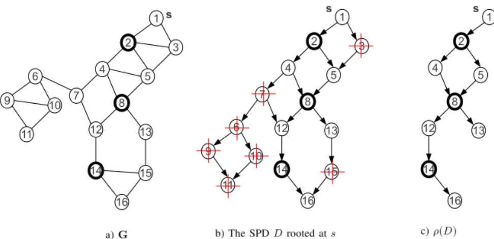
For example, in Figure 1.(b), vertices distinguished with a red ’+’ aremarkablevertices. Vertices030,070and0150are markable because they satisfy condition (1) of Definition 2, and vertices060,
090,0100and0110are markable because they satisfy condition (2)
of Definition 2.
Definition 3. LetDbe the SPD rooted ats∈V(G)andK⊂ V(G). Thepruned DAG of D with respect toK, denoted by
ρK(D), is the subgraph ofDinduced by{v∈V(D)|vis not markable}.
Figure 1.(c) shows the pruned DAG of the SPD presented in 1.(b), with respect toK={020,080,0140}.
LEMMA 2. Given a SPD D rooted ats ∈ V(G)and K ⊆ V(G),ρK(D)is computable inO(m).
The following properties can be shown forρK(D):
• if for a setKof vertices, the condition of Lemma 1 is satis-fied, none of the members ofKare markable, and therefore,
K⊆V(ρK(D)).
• if for a setKof vertices, the condition of Lemma 1 is satis-fied, for everyi: 1≤i≤ |K|,αD,K(i) =αρ(D),K(i). We
sometimes writeαD,K(i)orαρ(D),K(i)simply asαK(i).
• Forv∈V(D)∩V(ρ(D)),depD(v) =depρ(D)(v).
In the rest of this paper, we might talk about computing depen-dency scores either in a SPDD, or in its pruned formρ(D). To distinguish these two situations, we useδs•(A, D)for dependency score computation inDand δs•(A, ρ(D))for dependency score
computation inρ(D).sis a vertex in the network andAis either a ’vertex’ or ’a set of vertices’ or ’a sequence of vertices’.
LEMMA 3. Lets ∈V(G),K ⊆ V(G)\ {s}, andDbe the SPD rooted ats.
1. if members ofKare not in a single path ofD, then:δs•(K, D) =
0
2. if all members ofKare in a single path ofD, then: δs•(K, D) =δs•(αK(|K|), ρ(D)) (5) i.e. δs•(K, D) is equal to the number of shortest paths in ρ(D)fromsto other vertices which pass throughαK(|K|).
PROOF. Case (1) is directly resulted from Lemma 1. To prove case (2):
• First, we prove that for every shortest path in D starting formsand passing through all vertices inK, there exists a shortest path inρ(D)which starts fromsand passes through
αK(|K|). LetS=s1s2. . . slbe a shortest path froms1(=
s)toslinD which passes through all vertices inK. As a
contradiction, for any1< i≤l, supposesi ∈/V(ρK(D)).
Letsj∈Sbe the ancestor ofsiwith the largest depth which
belongs toV(ρK(D)). sj always exists becauses1 is an
ancestor ofsiands1∈V(ρK(D)).sjis not equal tosl
be-cause otherwise,Sis a path inρK(D). Now, considersj+1.
sj+1is notmarkablebecause:
– there does not exist a v ∈ Ksuch thatdepD(v) = depD(sj+1)becauseSpasses through all members of
K (andS can not pass through two vertices with the same depth). Therefore the first condition of Definition 2 does not hold forsj+1.
Figure 1: Part (a) shows a networkG. Kis{020,080,0140}, which are depicted with bold circles. Part (b) shows the SPD rooted at s=0 10. In this graph, vertices with red ’+’ aremarkablevertices with respect toK. We have:α(1) =020,α(2) =0 80,α(3) =0 140. Part (c) showsρK(D). As Lemma 3 says, the number of shortest paths inGstarting fromsand passing through all020,080and0140, is equal to the number of shortest path inρK(D)starting fromsand passing through0140.
– sjis not markable (since it belongs toV(ρK(D))) and sj+1is connected to it, therefore, the second condition
of Definition 2 does not hold forsj+1.
Therefore, a contradiction occurs becausesj+1is an
ances-tor ofsiwhich belongs toV(ρK(D))anddepD(sj+1) >
depD(sj). So,sibelongs toV(ρK(D)).
• Second, we prove that for every shortest path S in ρ(D) which starts fromsand passes throughαK(|K|), there exists
a shortest path inDwhich starts formsand passes through all vertices inK. SinceV(ρK(D))⊆V(D), vertices ofS
exist inDand we only need to show thatSpasses through all vertices inK. As a contradiction suppose that inD,Sdoes not pass through at least one vertexv∈K. Then, there will exist a vertexusuch thatu /∈K,depD(u) =depD(v)and S passes throughu. However, according to the first condi-tion of Definicondi-tion 2,uis markable and it can not be inρ(D) and therefore,Scan not pass through it.
Lemma 3 says that if we check the property expressed in Lemma 1 forK, and then, prune the network in the way defined in Defini-tion 3, instead of co-betweenness centrality computaDefini-tion ofK, we can compute betweenness centrality of a single vertex. This means that co-betweenness centrality computation of larger sets is not nec-essarily more difficult that co-betweenness centrality computation of smaller ones.
For example, in Figure 1,K ={020,080,0140}, vertices020,080 and0140 are in a single path of the SPD rooted ats =0 10 and
αK(1) =0 20,αK(2) =080andαK(3) =0140. αK(|K|) =0 140
and We have:δ010•,D({020,080,0140}) =δ010•,ρ(D)(0140).
Algorithm 1 shows the high level pseudo code for co-betweenness centrality computation of a setK. For a vertexs∈V(G)\K:
• First, the SPDDrooted atsis formed. Using e.g. the method of [7], this step can be done inO(m)time.
• Second, it is checked whether members ofKare in a single path ofD. To do so, the following steps are done:
1. For everyv∈ K,depD(v)is computed. This can be
done inO(m)time.
2. Vertices inKare sorted increasingly, according to their
depthinD. Using sorting algorithms likemerge sort
[19], this step can be done inO(|K|log|K|)time. 3. If two or more vertices have the samedepth, they are
not in a single path. Time complexity of this check is
O(|K|).
4. Letv1. . . v|K|be the members ofKwhich are sorted according to theirdepthinD. For everyj,1 ≤j ≤
|K|−1, the following procedure is performed: the sub-graph ofDinduced by
{vj} ∪ {u∈V(D)|uis a descendant ofvj}
is traversed in BFS, until either (i)vj+1is met or, (ii)
the traversal is finished. In case (i),vj+1is a
descen-dant ofvjand the procedure is performed forj+ 1. In
case (ii),vj+1is not a descendant ofvjand therefore,
all members ofKare not in a single path ofD. Mem-bers ofKare in a single path ofD, if and only if for allj, case (i) occurs. This procedure is done inO(m) time.
Therefore, it can be decided inO(m+|K|log|K|) time whether all members ofKare in a single path ofD. • Third,ρ(D)is computed. As Lemma 2 says, it can be
com-puted inO(m).
• Forth, the dependency score ofsonαD,K(|K|)inρ(D)is
computed. Using e.g. the method of [7], this step can be done inO(m)time.
The above mentioned procedure is performed for everys∈V(G)\
K. Therefore, we have the following theorem.
THEOREM 1. Algorithm 1 computes co-betweenness central-ity of a set K ⊂ V(G) in O(nm− |K|m+n|K|log|K| −
Algorithm 1High level pseudo code of the algorithm of computing vertex co-betweenness centrality.
1: VERTEXCOBETWEENNESS
2: Require.A network (graph)G, a setK⊆V(G). 3: Ensure.The co-betweenness centrality ofK. 4: CB←0;
5: for alls∈V(G)\Kdo
6: Generate the SPDDrooted ats;
7: ifall vertices inKare in a single path ofDthen
8: Computeρ(D) 9: cb←δs,•(αD,K(|K|), ρ(D)); 10: CB←CB+cb; 11: end if 12: end for 13: return CB;
3.1
Computing co-betweenness centrality of
se-quences
In this section, we investigate how the algorithm proposed for computation of co-betweenness centrality of sets can be revised to compute co-betweenness centrality of sequences.
LetK =v1, . . . , vkbe the sequence of vertices for which we
want to compute co-betweenness centrality. Lets∈V(G)andD
be the SPD rooted ats. There exists a shortest path fromsto some other vertext∈V(G)\ {s} \Kpassing through all vertices inK
in order (i.e. firstv1, secondv2etc), if in addition to the condition
presented in Lemma 1 (i.e. allvis are in a single path ofD), the
following holds:
∀i∈ {1, . . . , k} ⇒vi=αD,K(i) (6)
which means the order of vertices inKcorresponds to the order applied by the condition presented in Lemma 1. This condition makes computation of co-betweenness centrality easier; it is possi-ble to check both conditions inO(m)time as follows:
LetD be the SPD rooted at s ∈ V(G)\K. For everyvi, i∈ {1, . . . ,|K| −1}, the subgraph ofDinduced by{vi} ∪ {u∈ V(D) : uis a descendant ofvi}is traversed in BFS, until either
(i)vi+1is met, or (i) the traversal is finished. In case (i),vi+1is
a descendant ofvi. In case (ii),vi+1is not a descendant of vi,
and therefore, the conditions do not hold. The conditions presented in Lemma 1 and Equation 6 hold if and only if for allvis, case
(i) occurs. The procedure can be done inO(m)time, therefore it is possible to decide inO(m)time whether the conditions are satisfied. In fact, for sequences we do not need to compute the depth of vertices inD and sort members ofKaccording to their depth.
Similar to sets, in order to compute co-betweenness centrality of a sequenceK, for everys ∈V(G)\K, the following steps are done:
1. Form the SPDDrooted ats,
2. Check whether members ofK satisfy the conditions pre-sented in Lemma 1 and Equation 6,
3. ComputeρK(D)(if the conditions hold),
4. Calculateδs•(vk, ρK(D))(if the conditions hold).
Co-betweenness centrality ofKis the sum of the calculated de-pendency scores. All steps 1-4 can be done inO(m)time, and they are performed forn− |K|times, therefore, co-betweenness cen-trality of a sequence of vertices is computable inO(nm− |K|m) time:
THEOREM 2. Co-betweenness centrality of a sequenceK of vertices in an unweighted graph can be computed in O(nm−
|K|m)time.
3.2
Computation of co-betweenness centrality
in weighted graphs
Algorithms proposed for unweighted graphs can be used to pute co-betweenness centrality in weighted graphs. However, com-pared to unweighted graphs, time complexity of steps like forming SPDs, is higher for weighted graphs. As Corollary 4 of [7] says, for a weighted graphG, given a sources ∈ V(G), the number of all shortest paths to other vertices can be determined in time
O(m+nlogn).
For vertex co-betweenness centrality computation, this time com-plexity overcomes time comcom-plexity of checking whether all mem-bers of the set (or the sequence) are in a single path. This means that for weighted graphs, it is possible to compute co-betweenness centrality of a set (or sequence)Kof vertices inO((n− |K|)× (m+nlogn)) =O(nm− |K|m+n2logn− |K|nlogn)time. THEOREM 3. For weighted graphs, co-betweenness centrality of a set (or a sequence)Kof vertices is computable inO(nm−
|K|m+n2logn− |K|nlogn)time.
4.
CO-BETWEENNESS CENTRALITY
COM-PUTATION OF SETS OF EDGES
Betweenness of edges, defined in terms of the number of shortest paths passing through an edge, has many interesting applications in network analysis. For example, Girvan and Newman [16] used it to detect communities in complex networks. Very recently, Cuzzocrea et al. [10] proposed a new topology-control algorithm in wire-less sensor networks, called edge betweenness centrality, which is based on edge betweenness centrality.
Co-betweenness centrality of a set or a sequence of edges (edge co-betweenness centrality), is a generalization of this notion to a set or a sequence of edges. It has several applications in traffic network analysis, social networks etc. For example, an important problem in traffic data analysis is findinghot routesin a road network. Ahot routeis a sequence of edges which share (almost) the same amount of traffic. This problem has applications in city planning, real estate developing, etc and allows city-holders to better direct traffic or an-alyze congestion resources. Efficient algorithms for addressing this problem cluster sets of edges based on the density of common traf-fic they share [25]. With the assumption that movements are done through shortest paths, the basic element of this problem isedge co-betweenness centralitycomputation. A weight can be assigned to every edge (road) to reflect the number of trajectories passing through that edge. In the rest of this section, we first briefly for-mulate edge co-betweenness centrality, and then, we discuss about effective edge co-betweenness centrality computation.
4.1
Edge co-betweenness centrality
Fore ∈ E(G), σst(e)denotes the number of shortest paths
betweens and t that also pass throughe. We note that in this definition,sandtare allowed to be an end-point ofe. σst(W), W ⊆E(G), denotes the number of shortest paths betweensandt
that also pass (in any order) through all members ofW. We have
σs(e) = X t∈V(G)\{s} σst(e) and σs(W) = X t∈V(G)\{s} σst(W)
Betweenness centralityof an edgeeis defined as B(e) = X
s,t∈V(G)
σst(e)
Co-Betweenness centralityof a setW ⊆E(G)is defined as: CB(W) = X
s,t∈V(G)
σst(W)
We note that the number of shortest paths passing through a set of edges can be exponential in terms ofn.
4.2
Computation of edge co-betweenness
cen-trality
Lemma 4 expresses the necessary condition for a source vertex
s, to have at least one shortest path to other vertices in the network which pass through all edges inW:
LEMMA 4. Lets ∈ V(G), W ⊆ E(G)andDbe the SPD rooted ats. There exists at least one shortest path fromsto some other vertex in the network which pass through all edges inW, if vertices inLare in a single path ofD, whereLis
{v∈V(G)\ {s}|vis an end-point of at least onee∈W} (7) PROOF. The proof is omitted because it is similar to the proof of Lemma 1.
As a result of Lemma 4, we can define an ordering operatorα, in a way similar to Definition 1, which applies a total ordering on the members ofL, and therefore, on the members ofW. Dependency score ofs ∈ V(G)onW ⊆ E(G), i.e. the number of shortest paths fromsto other vertices in the network which pass through all edges inW, is defined asδs•(W) =Pt∈V(G)\{s}σst(W), and
thenCB(W) =Ps∈V(G)δs•(W).
Lemma 5 shows how ’edge co-betweenness centrality’ ofW is related to ’betweenness centrality’ of a single vertex inL.
LEMMA 5. Lets ∈ V(G), W ⊆ E(G)andDbe the SPD rooted ats.
1. ifW ⊆E(D)and members ofLare in a single path ofD, then:
δs•(W, D) =δs•(αL(|L| −1), ρL(D)) (8) whereLis defined in Equation 7.
2. otherwise:δs•(W, D) = 0
We note that inρL(D),αL(|L| −1, ρL(D))has always exactly
one child which isαL(|L|, ρL(D))and αL(|L|, ρL(D))has
al-ways exactly one parent which isαL(|L| −1, ρL(D)).
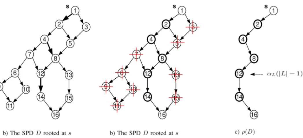
As an example, consider Figure 2. All members ofW which is {(010,020),(040,080),(0120,0140)}, are in a single path of the SPD Drooted ats. Furthermore,W ⊆E(D). Therefore,δs•(W, D) = δs•(0120, ρ(D))
Algorithm 2 shows the high level pseudo code of co-betweenness centrality computation for a set of edges. It differs from Algorithm 1 in two aspects. First, we need to check whetherW ⊆ E(D) (Line 7 of Algorithm 2). This step can be done inO(|W|)time since we can check inO(1)time whether there exists an edge be-tween two vertices of a graphG. Second, we need to perform the different steps (generating SPDs, checking whetherW ⊆ E(D), checking whether all members ofKare in a single path ofD, and
computing dependency scores) forntimes (the loop in Lines 5-14). We note that the second case increases time complexity of edge co-betweenness centrality, compared to vertex co-co-betweenness cen-trality computation.
THEOREM 4. Algorithm 2 computes co-betweenness centrality of a setW ⊂E(G)inO(nm+n|W|log|W|)time.
Algorithm 2High level pseudo code of the algorithm of computing co-betweenness centrality of a set of edges.
1: EDGECOBETWEENNESS
2: Require.A network (graph)G, a setW ⊆E(G). 3: Ensure.The co-betweenness centrality ofW. 4: CB←0;
5: for alls∈V(G)do
6: Generate the SPDDrooted ats; 7: ifW ⊆E(D)then
8: {let L be {v ∈ V(G) \
{s}|vis an end-point of at least onee∈W}} 9: ifall vertices inLare in a single path ofDthen
10: cb←δs•(αD,L(|L| −1), ρL(D)); 11: CB←CB+cb; 12: end if 13: end if 14: end for 15: return CB;
Co-betweenness centrality of a sequence W of edges can be computed, as the following. For every vetexsin the graph:
1. form the SPDDrooted ats, 2. check whetherW ⊂E(D),
3. check whether members ofLare in a single path ofD, 4. the condition expressed in item (3), applies a total ordering
on the edges inW. Check whether this total ordering is con-sistent with the order of edges in the sequence.
5. calculateδs•(αD,L(|L| −1), ρL(D)), if the conditions hold
(Lis defined in Equation 7).
Similar to our discussion for vertex co-betweenness centrality computation, we can show that every step 1-5 can be done inO(m) time. Therefore, we have the following theorem:
THEOREM 5. Co-betweenness centrality of a sequenceW of edges in an unweighted graph can be computed inO(nm)time2.
Finally, for co-betweenness centrality computation of a set (or a sequence) of edges in weighted graphs, we present the following theorem, where the proof is omitted because it is similar to the case of vertex co-betweenness centrality computation in weighted graphs.
THEOREM 6. For weighted graphs, co-betweenness centrality of a set (or a sequence)W of edges is computable inO(nm+
n2logn)time.
2A sequence of edges is also the sequence of vertices composing
the edges. What increases time complexity of co-betweenness cen-trality computation for edges is the number of source vertices used to form SPDs. According to the definitions, a shortest path starting with (or ending to) a member of a sequence of vertices does not contribute to the co-betweenness centrality of the sequence. How-ever, a shortest path starting with (or ending to) an end-point of a member of a sequence of edges contributes to co-betweenness cen-trality of the sequence.
Figure 2: Part (a) shows the SPD rooted ats=010.Wis{(010,020),(040,080),(0120,0140)}which are distinguished with bold lines. In part (b), members ofL={020,040,080,0120,0140}are distinguished with bold circles and vertices with red ’+’ aremarkablevertices with respect toL. We have:α(1) =020,α(2) =040,α(3) =080,α(4) =0120,α(5) =0140. Part (c) showsρL(D).
Table 1: Summary of real-world networks.
Dataset # vertices # edges Reference
Advogato 6,551 51,332 [27] ego-facebook 2,888 2,981 [28] caida 26,475 53,381 [22] CA-HepTh 27,770 352,807 [23] Eva 8,343 6,726 [30] Odlis 2,909 18,419 [34] Dolphins 62 159 [26] dblp 12,591 49,793 [24]
5.
EXPERIMENTAL RESULTS
We performed extensive experiments on real-world networks from different domains to assess the quantitative and qualitative behav-ior of the proposed algorithm. The experiments were done on one core of a single AMD Processor 270 clocked at 2.0 GHz with 8 GB main memory and2×1MB L2 cache, running Ubuntu Linux 12.0. The program was compiled by the GNU C++ compiler 4.0.2 using optimization level 3. Table 1 summarizes specifications of our real-world networks.
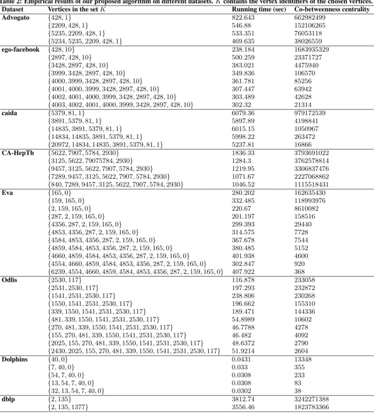
Due to lack of space, we only report the results obtained for co-betweenness centrality computation of a set of vertices. The results obtained for other problems, e. g. a set of edges, are very similar to the results reported here for a set of vertices. In our experiments, for every dataset, we select a random setPof vertices such that the subgraph induced by them is a path. Then, we start with a randomly chosen subsetKofP(of size 2) and compute their co-betweenness centrality. Then, we add a randomly chosen vertexv ∈ P \K
toKand compute co-betweenness centrality of the vertices inK. Adding new vertices toKis continued until co-betweenness cen-trality of all vertices inPis computed. We note that if the subgraph induced byKis a cyclic graph, its co-betweenness centrality will be0.
Two well-known existing methods in the literature are the algo-rithm of Kolaczyk et. al. [20] and the algoalgo-rithm of Dolev et. al. [11]. As mentioned earlier, the first one can only computes co-betweenness centrality of sets of size 2. On the other hand, the algorithm of Dolev et. al. can only compute co-betweenness cen-trality of sequences. Therefore, both algorithms are improper for
our comparisons since they consider limited cases. Thus, we only report the results of our algorithm. Table 2 reports the empirical results.
The first dataset studied here is theAdvogatonetwork3. It is the trust network of the Advogato online community. Vertices are users of Advogato and edges represent trust relationships [27]. Clearly, by increasing the size ofK, co-betweenness centrality decreases, i.e. for a subsetK0ofK, co-betweenness centrality ofK0 is not less than co-betweenness centrality ofK. This is reflected in our experiments. On the other hand, over Advogato, as the size ofK
increases, the time required to compute co-betweenness centrality decreases. It shows the efficiency of the SPDs pruning techniques. The next dataset is theego-facebook network4. This network
contains Facebook user-user friendships. A vertex represents a user and an edge indicates a friendship relationship [28]. As depicted in Table 2, over this dataset, co-betweenness centrality always de-creases as the size ofKincreases. On the other hand, the running time usually decreases, as the size ofKincreases. The only ex-ception is that the time required to compute co-betweenness cen-trality of{428,10}is less than the time required to compute co-betweenness centralities of{2897,428,10}and{3428,2897,428,10}. In these situations, while compared to smaller sets, forming pruned SPDs with respect to larger sets is much more expensive, shortest path counting over pruned SPDs of larger sets is not much more ef-ficient. In other words, the time required to prune SPDs dominates the speed-up resulted by counting shortest paths over pruned SPDs. The next dataset comes from autonomous systems of the Inter-net5. Thecaidanetwork is the undirected network of autonomous systems of the Internet connected with each other from the CAIDA project, collected in 2007. Vertices are autonomous systems (AS) and edges are communications [22]. Over this dataset, the run-ning time does not stay consistent as the size ofKchanges. For example, the running time increases when vertex14835is added to{3891,5379,81,1}. The next dataset is CA-HepTh6. This col-laboration network covers scientific colcol-laborations between authors papers submitted to High Energy Physics - Theory category. If an
3http://konect.uni-koblenz.de/networks/ advogato 4 http://snap.stanford.edu/data/ egonets-Facebook.html 5 http://snap.stanford.edu/data/as-caida.html 6 http://snap.stanford.edu/data/ca-HepTh.html
Table 2: Empirical results of our proposed algorithm on different datasets.Kcontains the vertex identifiers of the chosen vertices. Dataset Vertices in the setK Running time (sec) Co-betweenness centrality
Advogato {428,1} 822.643 662982499 {2209,428,1} 546.88 152106265 {5235,2209,428,1} 533.351 76053118 {5234,5235,2209,428,1} 469.635 38026559 ego-facebook {428,10} 238.184 1683935329 {2897,428,10} 500.259 23371727 {3428,2897,428,10} 383.021 4475940 {3999,3428,2897,428,10} 349.836 106570 {4000,3999,3428,2897,428,10} 361.781 85256 {4001,4000,3999,3428,2897,428,10} 307.447 63942 {4002,4001,4000,3999,3428,2897,428,10} 303.489 42628 {4003,4002,4001,4000,3999,3428,2897,428,10} 302.32 21314 caida {5379,81,1} 6079.36 979172539 {3891,5379,81,1} 5897.89 4198841 {14835,3891,5379,81,1} 6015.15 1050967 {14834,14835,3891,5379,81,1} 5998.22 263472 {20972,14834,14835,3891,5379,81,1} 5237.81 16866 CA-HepTh {5622,7907,5784,2930} 1836.33 3793691022 {3125,5622,79075784,2930} 1284.3 3762578814 {9457,3125,5622,7907,5784,2930} 1219.95 3306837476 {7289,9457,3125,5622,7907,5784,2930} 1071.67 2227068862 {840,7289,9457,3125,5622,7907,5784,2930} 1046.52 1115518431 Eva {165,0} 280.202 162635430 {159,165,0} 332.485 118993976 {2,159,165,0} 220.67 8610082 {287,2,159,165,0} 201.197 158516 {4356,287,2,159,165,0} 299.393 29440 {4853,4356,287,2,159,165,0} 314.575 7728 {4584,4853,4356,287,2,159,165,0} 367.678 7544 {4859,4584,4853,4356,287,2,159,165,0} 380.485 5152 {4660,4859,4584,4853,4356,287,2,159,165,0} 401.938 4600 {4554,4660,4859,4584,4853,4356,287,2,159,165,0} 302.847 920 {6239,4554,4660,4859,4584,4853,4356,287,2,159,165,0} 407.922 368 Odlis {2530,117} 116.878 233058 {2531,2530,117} 197.293 232872 {1541,2531,2530,117} 238.806 230268 {1550,1541,2531,2530,117} 196.662 155310 {339,1550,1541,2531,2530,117} 189.471 144336 {481,339,1550,1541,2531,2530,117} 54.8989 10602 {270,481,339,1550,1541,2531,2530,117} 46.7788 4278 {155,270,481,339,1550,1541,2531,2530,117} 46.482 4092 {2025,155,270,481,339,1550,1541,2531,2530,117} 48.6372 2790 {2430,2025,155,270,481,339,1550,1541,2531,2530,117} 51.9214 2604 Dolphins {40,0} 0.0431 13348 {7,40,0} 0.033 355 {54,7,40,0} 0.0308 233 {13,54,7,40,0} 0.0308 83 {32,13,54,7,40,0} 0.0302 38 dblp {2,135} 3812.74 3242271388 {2,135,1377} 3556.46 1823783366
authorico-authored a paper with authorj, an edge is drawn be-tween verticesiand j[23]. Over this dataset, the running time always decreases, as the size ofKincreases.
Eva is a prototype system for extracting, visualizing, and ana-lyzing corporate ownership information as a social network. Ap-plying the system to the telecommunications and media industries, Norlen et al. [30] constructed an ownership network with 6,726 re-lationships among 8,343 companies7. In this network, an edge from
companyuto companyvis drawn iff the companyuis an owner of companyv. Since we do not have ownership relationships for all companies, there will be companies without edges. Analysis shows that this network is highly clustered, with over50%of all compa-nies connected to one another in a single component. We tested our proposed algorithm over this ownership network. In this dataset, co-betweenness value of a set shows its impact on the ownership re-lations in the network. Our proposed algorithm scales well on this dataset, as sets with different sizes have close running times. By increasing the size of the set, its co-betweenness score decreases.
Odlis [34] is a hypertext reference system for users like library and information science professionals and university students and faculty. Users can add a new term to the system if they expect to encounter it in future or if they require to know its meaning. In the network representing this system, vertices are terms and an edge from termuto termvexists iff in the Odlis dictionary the termvis used to describe the meaning of termu8. As reflected in Table 2, over this network, in most cases, by increasing the size of the set the time required to compute its co-betweenness centrality decreases. In this network, the co-betweenness score of a setK shows the number of pairs of terms which use all terms inKto describe their meaning.
We also tested the proposed algorithm on a small dataset. The dolphins dataset [26] consists of an undirected graph of frequent as-sociations between 62 dolphins in a community living off Doubtful Sound, New Zealand9. In this dataset, the co-betweenness value
of a setKof dolphins shows the importance of all members inK
with together in associations between dolphins. As depicted in Ta-ble 2, over this dataset, sets with different sizes have almost the same running time.
Finally, we performed experiments on the dblp dataset10. Each vertex in this network is a publication (paper, book, etc), and each edge represents a citation of a publication by another publication [24]. Using the proposed algorithm, we calculated co-betweenness scores of two sets of vertices{2,135}and{2,135,1377}. As pre-sented in Table 2, it takes a shorter time to compute co-betweenness score of the larger set.
6.
RELATED WORK
Betweenness centrality is widely used as a precise indicator for the information flow controlled by a vertex in social and infor-mation networks [35]. It assumes that inforinfor-mation flow is done through shortest paths. Brandes [7] introduced new algorithms for computing betweenness centrality of a vertex, which is per-formed inO(nm)andO(nm+n2
logn)time for unweighted and weighted networks, respectively. Holme [17] showed that between-ness centrality of a vertex is highly correlated with the fraction
7 http://vlado.fmf.uni-lj.si/pub/networks/ data/econ/Eva/Eva.htm 8 http://vlado.fmf.uni-lj.si/pub/networks/ data/dic/odlis/Odlis.htm 9 http://www-personal.umich.edu/~mejn/ netdata/ 10http://konect.uni-koblenz.de/networks/ dblp-cite
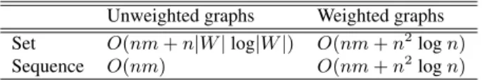
Table 4: Time complexity of edge co-betweenness centrality computation (|W|is the size of the set (sequence)).
Unweighted graphs Weighted graphs Set O(nm+n|W|log|W|) O(nm+n2logn)
Sequence O(nm) O(nm+n2
logn)
of time that the vertex is occupied by the traffic of the network. Barthelemy [3] showed that many scale-free networks [1] have a power-law distribution of betweenness centrality. There are also several notions of betweenness centrality which are used to deter-mine the structural prodeter-minence of Web pages [18] and [9].
There are several variations of betweennes centrality which are not designed for shortest path routing.Flow betweenness[15] equally considers all paths for routing. Borgatti [4] and [5] considered be-tweenness for all possible paths, as well as all possible trails, as well as walks (weighted inversely by length). He used numerical simulation to estimate the betweenness values. Newman [29] pro-posedRandom walk betweennesswhich prefers shorter paths over the longer ones. In this work, Newman provided closed-form equa-tions for the case of random traversal via walks. Borgatti [5] pro-posed a dynamic model-based view of centrality that focuses on the outcomes of vertices in a graph.
In [13], Freeman defined group betweenness centrality as a mea-sure of homogeneity of betweenness of members. Everett and Bor-gatti [12] defined group betweenness centrality as a natural exten-sion of betweenness centrality for sets of vertices. The other natu-ral extension of betweenness centnatu-rality isco-betweenness centrality
[20]. The authors of [20] presented an algorithm for individual co-betweenness centrality computation. However, this method works only for sets of size 2 and its time complexity isO(n3). Puzis et
al. [32] proposed aO(|K|3)time algorithm for computation of successive group betweenness centrality. In [33], the authors pre-sented two algorithms for finding the most prominent group. The first algorithm is based on heuristic search and the second is based on iterative greedy choice of vertices. In [11], the authors defined the Routing Betweenness Centrality (RBC) measure and presented algorithms for computing RBC of single vertices in the network and algorithms for computing group RBC of sets (or sequences) of vertices. Ballester et al. [2] discussed the importance of finding the key group in a criminal network. Borgatti elaborated in [6] on a Key Player Problem (KPP) that is strongly related to the cohesion of a network. He defined two problems: KPP-Pos and KPP-Neg. The solution of the first problem is a group maximally connected to all other vertices in a graph and the solution of the second is a group maximally disrupting the network.
7.
CONCLUSION
In this paper, we developed efficient algorithms for vertex and edge co-betweenness centrality computation in different settings. Tables 3 and 4 summarize time complexity of the proposed meth-ods. Our methods are based on reducing vertex co-betweenness centrality and edge co-betweenness centrality of a set (or a se-quence) tobetweenness centralityof a single vertex. They are not limited to special cases and they are more efficient than existing methods. We empirically evaluated the efficiency of the proposed methods and showed their high performance over different real-world networks.
8.
REFERENCES
[1] A.-L. Barabasi and R. Albert, Emergence of scaling in random networks, Science, 286, 509-512, 1999.
Table 3: Time complexity of vertex co-betweenness centrality computation (|K|is the size of the set (sequence)).
Unweighted graphs Weighted graphs
Set of vertices O(nm− |K|m+n|K|log|K| − |K|2log|K|) O(nm− |K|m+n2logn− |K|nlogn)
Sequence of vertices O(nm− |K|m) O(nm− |K|m+n2logn− |K|nlogn)
[2] C. Ballester, A. C. Armengol and Y. Zenou, Who’s who in networks. wanted: The key player, Econometrica, 74(5), 1403-1417, Sep. 2006.
[3] M. Barthelemy, Betweenness centrality in large complex networks. The Europ. Phys. J. B - Condensed Matter 38, 2(Mar.), 163-168, 2004.
[4] S. P. Borgatti, Types of network flows and how to destabilize terrorist networks, Sunbelt International Social Networks Conference, New Orleans, 2002.
[5] S. P. Borgatti, Centrality and network flow, Social Networks, 27(1), 55-71, 2005.
[6] S. P. Borgatti, Identifying sets of key players in a social network, Comput. Math. Organ. Theory, 12(1), 21-34, 2006. [7] U. Brandes, A Faster Algorithm for Betweenness Centrality. Journal of Mathematical Sociology, 25(2), 163-177, 2001. [8] U. Brandes, On variants of shortest-path betweenness
centrality and their generic computation, Social Networks, 30(2), 136-145, May 2008.
[9] S. Brin, R. Motwani, L. Page and T. Winograd, What can you do with a web in your pocket? IEEE Bulletin of the Technical Committee on Data Engineering, 21(2), 37-47, 1998. [10] A. Cuzzocrea, A. Papadimitriou, D. Katsaros and Y. Manolopoulos, Edgebetweenness centrality: A novel algorithm for QoS-based topology control over wireless sensor networks, Journal of Network and Computer Applications, 35(4), 1210-1217, July 2012.
[11] S. Dolev, Y. Elovici and R. Puzis, Routing betweenness centrality, J. ACM, 57(4), 2010.
[12] M. Everett and S. Borgatti. The centrality of groups and classes, Journal of Mathematical Sociology, 23(3), 181-201, 1999.
[13] L. C. Freeman, A set of measures of centrality based upon betweenness, Sociometry, 40, 35-41, 1977.
[14] L. C. Freeman, Centrality in social networks: Conceptual clarification. Social Networks, 1(3), 215-239, 1979.
[15] L. C. Freeman, S. P. Borgatti, and D. R. White, Centrality in valued graphs: A measure of betweenness based on network ïˇn ´Cow, Social Networks, 13(2), 141-154, 1991.
[16] M. Girvan and M. E. J. Newman, Community structure in social and biological networks, Proc. Natl. Acad. Sci. USA 99, 7821-7826, 2002.
[17] P. Holme, Congestion and centrality in traffic flow on complex networks, Adv. Complex Syst, 6(2), 163-176, 2003. [18] J. M. Kleinberg, Authoritative sources in a hyperlinked
environment, Journal of the Association for Computing Machinery, 46(5), 604-632, 1999.
[19] D. Knuth, Section 5.2.4: Sorting by Merging, Sorting and Searching. The Art of Computer Programming 3 (2nd ed.), Addison-Wesley, 158-168, 998.
[20] E. D. Kolaczyk, D. B. Chua and M. Barthelemy.
Group-betweenness and co-betweenness: Inter-related notions of coalition centrality, Social Networks, 31(3), 190-203, 2009.
[21] S. Lammer, B. Gehlsen, D. Helbing. Scaling laws in the spatial structure of urban road networks. Physica A, 363(1), 89-95, 2006.
[22] J. Leskovec, J. Kleinberg and C. Faloutsos, Graphs over Time: Densification Laws, Shrinking Diameters and Possible Explanations, KDD, 2005.
[23] J. Leskovec, J. Kleinberg and C. Faloutsos, Graph Evolution: Densification and Shrinking Diameters, ACM Transactions on Knowledge Discovery from Data (ACM TKDD), 1(1), 2007. [24] M. Ley, The DBLP computer science bibliography:
Evolution, research issues, perspectives, In Proc. Int. Symposium on String Processing and Information Retrieval, 1-10, 2002.
[25] X. Li, J. Han, J.-G. Lee and H. Gonzalez, Traffic
density-based discovery of hot routes in road networks, 10th Symposium on Spatial and Temporal Databases (SSTD), 441-459, 2007.
[26] D. Lusseau, K. Schneider, O. J. Boisseau, P. Haase, E. Slooten, and S. M. Dawson, The bottlenose dolphin community of Doubtful Sound features a large proportion of long-lasting associations, Behavioral Ecology and
Sociobiology 54, 396-405, 2003.
[27] P.Massa, M. Salvetti and D. Tomasoni, Bowling alone and trust decline in social network sites, In Proc. Int. Conf. Dependable, Autonomic and Secure Computing, 658-663, 2009.
[28] J. McAuley and J. Leskovec, Learning to discover social circles in ego networks, NIPS, pages 548-556. 2012. [29] M. E. J. Newman, A measure of betweenness centrality
based on random walks, Social Networks, 27(1), 39-54, 2005. [30] K. Norlen, G. Lucas, M. Gebbie and J. Chuang, EVA:
Extraction, Visualization and Analysis of the Telecommunications and Media Ownership Network. Proceedings of International Telecommunications Society 14th Biennial Conference (ITS2002), Seoul Korea, August 2002.
[31] A. Perer, B. Shneiderman, Balancing systematic and flexible exploration of social networks, IEEE Transactions on Visualization and Computer Graphics, 12(5), 693-700, 2006. [32] R. Puzis, Y. Elovici and S. Dolev. Fast algorithm for
successive computation of group betweenness centrality, Phys. Rev. E, 76(5), 2007.
[33] R. Puzis, Y. Elovici and S. Dolev, Finding the most prominent group in complex networks, AI Commun. 20(4), 287-296, 2007.
[34] J. M. Reitz, ODLIS: Online Dictionary of Library and Information Science, 2002.
[35] G. Yan, T. Zhou, B. Hu, Z. Q. Fu, and B.-H. Wang, Efficient rout-ing on complex networks. Phys. Rev. E, 73, 046108, 2006.