Agglomeration economies with consistent productivity estimates

BGPE Discussion Paper

No. 113

Agglomeration economies with consistent

productivity estimates

Philipp Ehrl

December 2011

Editor: Prof. Regina T. Riphahn, Ph.D.

Friedrich-Alexander-University Erlangen-Nuremberg © Philipp Ehrl

Agglomeration economies with consistent productivity

estimates

This paper investigates the relative impact of microeconomic agglomeration mech-anisms on plant’s total factor productivity (TFP) using German establishment and employment level data. Contrasting different strategies to estimate TFP from plant level production functions reveals that not accounting for the endogeneity of input choices and not separating price effects from true productivity leads to underesti-mated agglomeration economies. Under the preferred TFP measure, labor market pooling, captured by the correlation of the occupational composition between one county-industry and the rest of the county, is found to have the largest impact. Be-sides, two knowledge spillover mechanisms, transmitted via job changes and public R&D funding, positively affect plant productivity. Except for job changes the result is even robust when the spatial units are broadened from counties to labor market re-gions. Testing for urbanization and localization economies, I find that TFP is higher in more specialized and larger counties, whereas sectoral diversity is of no importance at the county level.

JEL-Classification: D24, R11, R30

Keywords: agglomeration economies, modifiable areal unit problem , TFP estimation, price bias, localization, urbanization economies

∗

I would like to thank Rainald Borck, Wolfgang Dauth, Malte Mosel, Steffen Müller, Michael Pflüger and seminar participants at the University of Passau, 4th User Conference of the RDC, GfR Summer Conference in Dresden, UEA at the ERSA in Barcelona and VfS in Frankfurt for fruitful discussions and comments. Furthermore, I thank the Research Data Center (RDC) of the German Federal Employment Agency at the Institute for Employment Research for the data access, especially Mathias Dorner, Daniela Hochfellner and Dana Müller for their support. The data basis of this publication is the Employment Panel (IABB, years 2000-2007) and the Employment Panel (BAP, years 2000-2007). Data access was via guest research spells at the FDZ and via controlled data remote access. Contact: philipp.ehrl@uni-passau.de, University of Passau, Innstr. 27, 94032 Passau, Germany.

1

Introduction

Despite higher factor prices for land and labor economic activity is spatially concentrated1. But what exactly makes agglomerations more attractive than sparsely populated regions? More than a hundred years ago, Alfred Marshall (1890) described three motives, why firms locate close to each other: the proximity to their suppliers, a specialized local labor mar-ket and the presence of knowledge spillovers. Until today, regional scientists are concerned with a thorough examination of these agglomeration forces. Over the last three decades researchers have developed different microeconomic foundations for Marshall’s anecdotal evidence2. Yet, concerning the empirical evidence, Glaeser and Gottlieb (2009: 985) note that "the field has still not reached a consensus on the relative importance of different sources of agglomeration economies". The few studies that are concerned with the assess-ment of their relative importance differ largely in the dependent variable at use. Puga (2010: 204) argues that productivity is the "most direct approach" in order to capture agglomeration economies. In fact, examining employment growth or concentration may suggest that Marshall’s forces are beneficial to firms3. However, unlike total factor pro-ductivity (TFP), these approaches are silent about the exact nature of the benefit4.

The present study sets itself apart from the preceding literature along three dimensions. It is the first study that quantifies the relative importance of different microeconomic ag-glomeration mechanisms according to their impact on TFP. To this end, TFP is estimated from plant level production functions and proxies for labor pooling, input relations and knowledge spillovers are constructed, following closely the predictions from theoretical models. The second point is methodological: I discuss, how different estimation strategies for TFP influence the resulting agglomeration economies. Thirdly, I show how the range of industries and the modifiable areal unit problem (MAUP) influences the results. The MAUP refers to the trouble that aggregate values in any spatial analysis can be artifacts from the accidental delineation of its boundaries. Using these methods, the present paper also adds to the ongoing debate about whether localization or urbanization economies are beneficial to firms (Beaudry and Schiffauerova 2009).

Discriminating between different forces is complicated due to their ’Marshallian equiv-alence’ (Duranton and Puga 2004). That is, most theoretical models on agglomeration mechanisms share the prediction that the benefits grow in the number of workers or firms. Indeed, earlier contributions have used the size (Sveikauskas 1975) or density of areas (Ci-ccone and Hall 1996) as proxies, leaving open how the agglomeration benefits are actually transmitted to firms. That is why, I collect unique features in micro-founded models and

1

For evidence from elaborated concentration indices see Duranton and Overman (2005) for the UK and Koh and Riedel (2009) for Germany.

2

Duranton and Puga (2004) provide a comprehensive survey of this literature.

3_{In this context Cingano and Schivardi (2004) compare regressions with TFP growth and employment} growth as the dependent variable. They find positive coefficients for the size and specialization of a region in TFP growth regressions but the opposite result with employment growth.

4

Of course, firms base their location choice on expected profits rather than on expected productivity. Therefore besides TFP differences cost advantages or higher demand in agglomerations may coexist, but these influences are much harder to trace than TFP.

combine several data sets to construct proxy variables at the county level (NUTS 3 level). As argued above, TFP is the most direct and telling indicator to measure agglomeration advantages at the firm level. Presumably due to data constraints, only a small fraction of studies draws inference from TFP5. Besides, its estimation is quite complex, as the sizable literature on this topic documents, see e.g. Ackerberg et al. (2007). I account for the correlation of input choices with current productivity levels using the Olley and Pakes (1996) (OP henceforth) procedure. Due to this simultaneity the plant’s TFP affects the input choice, which translates into biased coefficients and a biased TFP estimate. Furthermore, I correct for unobserved output prices as proposed in Klette and Griliches (1996), which allows one to separate true productivity from demand side effects. Having revenues instead of real output as the dependent variable in the production function means that plant’s prices appear in the equation. Without the adjustment the price remains in the residual and is thus erroneously contained in the TFP measure. It will be shown that the estimation technique makes a difference with regard to the significance level and magnitude of agglomeration mechanisms. So far, only De Loecker (2011), Del Gattoet al.(2008) and Muendler (2007) have corrected jointly for the simultaneity bias and the omitted price bias, but none of them has taken the TFP estimates into a regional analysis. To this end the procedure is modified to accommodate the influence of agglomeration variables on TFP and an additional selection bias, as originally proposed by OP.

To overview the integration of the present paper in the literature, existing studies on agglomeration economies can be classified in two categories. Those that analyze TFP and those that aim at the discrimination between agglomeration forces. The majority in the first category, e.g. Henderson (2003), Combes et al. (2010), Martin et al. (2011), look at measures of concentration and urbanization economies but not at distinct agglomera-tion mechanisms. Yet, with more refined TFP measures, an elaborate robustness analysis and the look at another country the present study contributes to this ongoing research. Section 5.5 discusses my findings in the light of the prior results. There is one exception which relates several agglomeration mechanisms to TFP. Greenstoneet al.(2010) provide evidence that labor market pooling and knowledge spilloversseparately generate external-ities, however they fail to do so in a multivariate setting. Of course, just in the latter case can we compare their relevance. Another distinction to their study are the location specific agglomeration proxies used here and the inclusion of non-manufacturing sectors, as is rarely the case. Rigby and Essletzbichler (2002) and Baldwinet al.(2010) are studies in the second category, who find that all three Marshallian forces simultaneously have a positive effect on labor productivity. Still, these studies do not compare their magnitude and as will be clear below, I argue that labor productivity is not a particularly reliable measure. Their measure for input-output relations is very similar to the one I use, but their remaining two agglomeration proxies are less specific. Then again, Baldwinet al. (2010) are more careful about regional fixed effects and reverse causality. Ellison et al. (2010)

5

See Rosenthal and Strange (2004), Puga (2010) and Glaeser and Gottlieb (2009) for surveys on the empirics of agglomeration economies.

study the co-agglomeration of similar industries and also reveal that all three Marshallian forces exert positive influence, with input-output relations being the most important.

Using establishment and employment level data from the Institute for Employment Research (IAB) from 2000 to 2007, I find that in univariate regressions all agglomeration mechanism variables have the expected sign and statistical significance. However, some variables’ significance vanishes in multivariate regressions. Still, labor pooling, captured trough the correlation of the occupational composition between one county-industry and the rest of the county, has the highest and most significant impact on plant productivity. Besides, two knowledge spillover mechanisms, transmitted via job changes and public R&D funding, positively affect plant TFP. The poor performance of input linkages may be due to the lack of detailed information about the flow of intermediate goods. In both multivariate and univariate regressions the agglomeration externalities tend to be more significant and higher in magnitude, when the omitted price and endogeneity bias are accounted for. On the one hand, it confirms the theoretical (Melitz 2003) and empirical (Foster et al.

2008) finding that highly productive establishments set lower prices. This, on the other hand, stresses the importance of separating price effects from true productivity. The robustness of these results is evaluated by controlling for the type of county and varying the range of industries. Then, the spatial unit of the entire analysis is changed from counties to larger labor market regions in order to assess the MAUP and the geographic scope of the externalities. Furthermore, I construct four additional productivity measures: labor productivity, TFP estimated from value added instead of revenue based production functions, and TFP resulting from the Levinsohn and Petrin (2003) and the Ackerberget al.

(2006) estimation procedure, as alternatives to the OP model. The comparison suggests that especially labor productivity is an imprecise measure, which is likely to overestimate the size and significance of agglomeration economies. In a nutshell, the key findings remain valid under these extensions.

Concerning the discussion about externalities from the local industrial environment, no significant sign is found for a diversified industrial structure, as suggested by Jane Jacobs (1969). Only when the size of the spatial units is broadened, diversity has a small but significant impact. Throughout, the data shows that localization proxies are beneficial to plant’s productivity and average productivity is higher by about 0.2%, when the employment size of a county is increased by 10%. This result is within the range of previous studies from other countries that also draw inference from TFP, e.g. Henderson (2003) and Combeset al. (2010).

The remainder of the paper is organized as follows. The next section lays out the TFP estimation strategy. Section 3 describes the data and the construction of the agglomeration variables. Estimation results are presented in section 4. Section 5 provides extensive robustness checks and a discussion of the findings with respect to the urbanization and localization debate. Section 6 concludes the paper.

2

TFP estimation

2.1 Estimation difficulties

Before presenting the estimation strategy used in the paper, this section reviews some of the difficulties in estimating production functions. Subsequently, I describe, how they are incorporated in order to obtain a consistent productivity measure. The conventional starting point is the Cobb-Douglas technology in logarithmic form

yjt=ajt+αkkjt+αlljt+αmmjt+ζzjt+upjt (1)

whereyjtis output of firm6jin periodt,αxwithx={k, l, m}is the production elasticity of

capital, labor and intermediate inputs, andup_jt is an unobserved i.i.d. shock to production. The termzjt represents controls in the production function, which are a dummy variable

for firms located in West Germany, industry fixed effects and the firm’s share of high skilled workers. Total factor productivity ajt can be split up in two terms: ajt = β0+ωjt. The

first one,β0, can be interpreted as common stock of technology or an efficiency level shared by all firms. ωjt is the firm specific part of TFP7, being unobserved by the researcher but

known to firm.

Two well known problems plague the estimation of production functions: the trans-mission bias and the omitted price bias. The first problem arises, because the current productivity level influences the decision about optimal input usage8. Klette and Griliches (1996) prove that the direction of the transmission bias is strictly positive. Thus when adjusting for this bias, we expect lower scale elasticity estimates αx. Several strategies

have been proposed to overcome this problem9. Probably the most prominent is the con-trol function approach in Olley and Pakes (1996). Its basic idea is that firm’s productivity also influences other decisions, for example investments ijt, i.e. ijt(ωjt). Inversion of this

function allows us to replace the unknownωjt from the production function. I also discuss

the results from other estimation strategies in the robustness section, but OP turned out to be the most appropriate and reliable.

The omitted price bias arises due to the fact that in theory the LHS variable in the production function is output measured in quantities. Unfortunately, there are only few data sets, where this information is given. Usually firms report their output in monetary units, which means that the firm’s log pricepjt has to be added to both sides of equation

(1). Prior studies have typically proxiedpjtby an industry level deflator or have completely

ignored the problem. If firm prices were to depart systematically from the average price level of the industry, regression coefficients will be biased. Theoretical models featuring firm heterogeneity, like Melitz (2003), tell us, that the most productive firms set below average

6_{Even though the study is based on establishment specific data I use the term ’firm’ interchangeably.} 7

Henceforth the terms TFP and likewise productivity only refer to this firm specific part ωjt, unless explicitly stated.

8_{Deriving optimal input demand functions from (1) shows their dependence on productivity.} 9

prices, sell above average quantities and consequently use more of the production factors. Hence downward biased regression coefficients can be expected from estimation of equation (1)10. Foster et al. (2008) make use of a dataset with information on output in physical quantities and revenues, confirming that revenue based productivity estimates embody price variation. Consequently, inference from revenue based and physical productivity estimates is different. When presenting the estimation results, I will also discuss the outcomes without adjustments for the endogeneity and omitted price bias.

2.2 Identification strategy

This section outlines how the two presented biases are taken into account, in order to derive consistent TFP estimates. First, I make use of a specific demand system to tackle the omitted price bias. Then, a model of industry dynamics is introduced, which allows to implement the control function for unobserved TFP. Only De Loecker (2011), Del Gatto

et al.(2008) and Muendler (2007) have already applied a combination of these two estima-tion procedures from Klette and Griliches (1996) and OP. I also control for an addiestima-tional selection bias, as proposed in the original OP framework, but not adopted by the above cited studies. The main novelty here is the application to regional data and consequently allowing the productivity variable to be influenced by some agglomeration variables Gc. This has consequences for the inversion of the control function and the survival probability used to control for the selection bias.

The production function with output in terms of log revenuerjt in fact is given by

rjt=yjt+pjt =ajt+αkkjt+αlljt+αmmjt+ζzjt+up_jt+pjt (2)

To replace unobserved firm level prices pjt, I rely on the CES demand function from the

Dixit and Stiglitz (1977) framework11. UsingrIt=pIt+qIt, its logarithmic form is

qjt =−σ(pjt−pIt) +qIt+udjt (3)

where firm level demandqjt depends negatively on the firm’s own price and positively on an

aggregate demand shifterqItand an aggregate price indexpIt. σis the constant elasticity of

demand andud_jt are i.i.d. demand shocks. When it comes to the empirical implementation, the question is, which is the corresponding market toqIt, pIt? Two arguments suggest that

the industry segment of the national market is the most suitable approximation: (1) Given that the majority of exporting firms generate only a small percentage of their revenues abroad (Fryges and Wagner 2010), for most firms the national market is what matters. (2) Economic conditions on input and sales markets in all sectors implausibly follow the

10_{Klette and Griliches (1996) also discuss other influence channels that lead to a systematic negative} relation between prices and input factors.

11_{Despite its well known restrictiveness the CES demand is popular, simple and easily combined with} the Cobb-Douglas production function. Klette and Griliches (1996) and the above cited studies used the CES demand function, too.

same development over time. So taking one and the same price index and demand shifter for all firms, seems a rather crude proxy. To make the distinction between sectors clear, pIt, qIt andσ get the superscript ’s’ henceforth. Combining demand side information from

(3) with the production function in (2) yields

e rjt ≡yjt+pjt−psIt = = σs−1 σs (ajt+αkkjt+αlljt+αmmjt+ζzjt) + 1 σs(r s It−psIt) +ujt (4)

Both i.i.d. shocks ud_jt and up_jt are combined in ujt. Estimating this production function

with deflated revenues as the dependent variable circumvents the omitted price bias, while it also provides an estimate for the demand elasticity in industry sas a byproduct. Note that productivity_eajt ≡βe₀+ω_ejt = (σ

s₋₁

σs )(β0+ωjt)and the input elasticitiesαex≡(

σs₋₁

σs )αx

withx={K, L, M}are reduced form parameters, when estimated without adjustment for the omitted price bias.

Now,ωjtis the only remaining unobserved factor hindering consistent estimation of the

production function. Olley and Pakes (1996) introduce a model of firm behavior, which is described in more detail in Appendix A. Importantly, the model yields an investment demand equationijt =it(kjt, ωjt(Gct)). Given thatijt is monotonic in ωjt and the regional

factors are known exogenous state variables, inversion gives ωjt = ht(kjt, ijt, Gct). The

upper panel in figure A.1 in the Appendix confirms the latter assumption graphically. Replacing unobserved productivity in the production function in equation (4) by the control functionht(·) gives e rjt =βe₀+ e αlljt+αemmjt+ 1 σs(r s It−psIt) +φt(kjt, ijt, Gct) +ζzjt+ujt

where the unknown functionφt(kjt, ijt, Gct)≡αekkjt+eht(kjt, ijt, G

c

t) is approximated by a

second order polynomial. Due to multicollinearity problems α_ek has to be estimated in a

second stage. Its identification is based on the moment condition E[ξjt|kjt] = 0 derived

from the assumption that firm’s productivity follows an first order Markov process andξjt

is its exogenous innovation shock. Finally log composite TFP is residually collected from

ˆ ajt= " e rjt−αˆelljt−αeˆmmjt−αˆekkjt− ˆ 1 σs (rIt−pIt)−ζzˆ jt # _ˆ σs ˆ σs₋₁

3

Data

3.1 Plant and industry level data

For the estimation of the production functions the IAB Establishment Panel (IABB) is used from 2000 to 2007. The main advantage of this panel is that the location of a plant at NUTS 3 level (counties) and the industry classification are available. A more detailed de-scription of the IABB is given in Fischeret al.(2009) and Appendix B contains more on the

construction of the panel. The IABB provides information about revenues, intermediate inputs, investments, the number and qualification level of all workers, among others. Cap-ital input is constructed from plant investment behavior employing the modified perpetual inventory method according to Müller (2008).

As was made clear from the description of the estimation strategy above, the production function is combined with a specific demand system in order to replace unobserved plant prices by aggregate demand shifters and price indices. Since I have assumed that the relevant market is industry specific, aggregate revenues are an appropriate demand shifter. The necessary data is taken from the Federal Statistical Office. Table B.1 in the Appendix lists the 22 remaining industries and the respective number of observations without any missing values in all variables.

3.2 Regional data

Agglomeration economies result from some kind of transport cost saving (Ellison et al.

2010). Naturally, we would expect their strength to decay with distance. However, the spatial spread of influence may differ across the agglomeration channels. For example, a labor market advantage, based on the mobility of workers, is likely to extend over a larger geographical area than knowledge spillovers created through the incidental meeting of workers. I opted to take counties (the NUTS 3 level) as spatial units. In order to investigate the spatial decay and whether the choice of spatial units are decisive for the results, in the robustness section the analysis is repeated at the level of larger labor market regions. In 2007, Germany was divided into 423 counties12. Most of the information to construct agglomeration variables is taken from other data sources (as detailed below) and is then matched into the IABB via the industry and county identifiers.

3.2.1 Urbanization and localization

The FSO provides the square footage and the number of employees in each county for the 22 industries examined in this study. Furthermore, the total employment level in each county is taken from the Federal Employment Agency (BA). Based on this information the urbanization and localization variables are constructed as follows. Localization economies (or interchangeably specialization economies) are captured through the employment share of industry s in county c: Ecs Ec = Ec s P Ec

s. Beaudry and Schiffauerova (2009) advocate to

investigate, whether the absolute or the relative size of an industry is more important, which is why I also experiment with the employment level in a county-industry.

The urbanization hypothesis, often associated with the work of Jacobs (1969), predicts that a diverse industrial environment will foster productivity of all firms in that region. The construction of a diversity measure is not straightforward. Henderson (2003) used a

12

All districts that have undergone changes between 2000 and 2007 are aggregated, so that the area is consistent throughout these year. This is the case for districts in Saxony, the city of Hannover and Berlin.

comparison between the industrial structure of a countyc and the whole country jacobs1c=X s Ec_s Ec − Es E 2

where Es is total employment in industry s and E = PEs is the total of workers in

Germany13. If the employment shares of all industries s in a county mirror the national employment shares, this measure takes on the value of zero. In this case countycpossesses the maximum diversity. In fact, jacobs1 measures the lack of diversity, hence the urban-ization hypothesis predicts a negative coefficient. A second inverse measure of diversity (jacobs2) used is the employment share of the three largest industries in a county14_{. For}

comparisons with earlier studies, e.g. Combeset al. (2010) and Ciccone and Hall (1996), the log density and the log size (in terms of employment) of a region will also be employed in the productivity analysis.

Even though all of these regional variables capture agglomeration economies, they do not provide us with a notion of how productivity benefits are actually transmitted to plants. Duranton and Puga (2004) survey a wide range of models which provide differ-ent microeconomic foundations of agglomeration economics. All of them share the same prediction: large locations are beneficial to plants. The current challenge for empirical work is to discriminate between them. Since most of the models are based on two types of labor and only one or two sectors, some interpretation is necessary for the empirical implementation. Yet, I tried to align the variables’ construction as closely as possible to the underlying theory. In the center of attention of this investigation are the following microeconomic mechanisms, classified according to the famous three Marshallian labels.

3.2.2 Input-relations

In models with an intermediate goods sector, e.g. Ethier (1982), Abdel-Rahman and Fujita (1990), the production function of firms in the final goods sector exhibits external returns to scale in the number of intermediate goods producers. These models typically assume that assembling firms use all available intermediate goods. When we take this prediction to the empirical inquiry, we may want to be more realistic. In fact, some industries are heavily dependent on inputs from another industry or even from their own industry, while other sectors hardly exchange goods. Usually researchers have looked at both input and output linkages. In order to stick as close as possible to the underlying theory, only input flows are considered here. Introducing trade costs, as e.g. in Venables (1996), implies higher demand for local intermediate goods and in turn a higher contribution to the productivity of their local customers. For simplicity this investigation disregards interactions with neighboring

13

Note that all terms in the construction of jacobs1c vary by time, but are not explicitly denoted by a subscriptt to save on notation. This applies also in the construction of the following agglomeration variables.

14_{Glaeser et al. (1992) have used the share of the five largest industries in a city to capture Jacobs} economies. Note that in the construction ofjacobs2 only the 22 sectors considered in this investigation form the total county employment. This explains its large mean of 0.58, cf. table 1 below.

counties and focuses only on supplier relations within the own county.

The indicator for supplier relations in industryiis the amount of goods that industryi purchases from industryjrelative to all industryi’s inputs. Intra-industry transactions are considered as well. Because the range of industries are relatively broad, it is not surprising that intra-industry input shares are on average much larger than shares between different industries. These numbers provided by the FSO in the input-output-matrix, are used to construct the following indicator for the strength of input-output-relations. Regarding supplier relations within an industry, basic metals (0.64), chemical industry (0.57) and motor vehicles (0.48) rank on top. Between different industries the highest share of input usage is observed for sales from transportation/communication to wholesale/retail trade (0.33). Then this measure of linkage strength between industrysand all other industries u(strengthsu) is related to the industrial structure in each region as follows15

input-linkagec_s=X u strengthsu· E_uc Ec

According to the theory outlined above, this means that the measure for input-externalities rises in the relative size and the relative weight of the supplying sectors.

3.2.3 Labor market pooling

Coles and Smith (1998) provide a microeconomic foundation for labor market pooling. Their model is based on a frictionless labor market, where firms post their vacancies and unmatched workers apply for all of these posts. This framework generates a matching func-tion with increasing returns to scale in both the number of firms and workers. That means, a larger market provides more opportunities to find suitable matches and thus expected productivity is higher. For the empirical realization I compute the correlation between oc-cupations in the industry under scrutiny and all remaining ococ-cupations in a county16. This construction presumes that all firms from the same industry in a county have a common composition of staff. The closer the industry profile is to the composition of the local labor market, the less effort firms from that industry have in finding suitable employees. In this manner the variable is close to the original writing of Marshall (1890: 271): "a localized industry gains great advantage from the fact that it offers a constant market for skill. Em-ployers are apt to resort to any place where they are likely to find a good choice of workers with special skill which they require". The information about worker’s occupations per county is provided in the BA Employment Panel (BAP)17. The BAP is a sample of all

15_{Note that the normalization for the supplier measure is done with the amount of inputs from all} in-dustries. Ellisonet al.(2010) use a similar measure for input-relations, but their coagglomeration variables are industry specific. Rigby and Essletzbichler (2002) take both input and output linkages and weight them by location coefficients.

16

Conceptually similar variables are used in Ellisonet al.(2010), Baldwinet al.(2010) and Rigby and Essletzbichler (2002), however without location specific information about the distribution of occupations, as is the case here.

17_{The construction is based on the anonymized version of the 3-digit occupational classification of the} German Federal Employment Agency, which lists 282 different occupations.

employees subject to social security in Germany. It contains quarterly information about the occupation, education level, working place among others.

Another implementation of a labor pooling measure from Coles and Smith (1998) is to look at the average number of vacancies in each county. In order to get a better grip on the element of suitable worker qualifications, the variable only considers the vacancies for high skilled staff.

3.2.4 Knowledge spillovers

For the same reason as above, I will try three different proxies for knowledge spillovers. There is no unified framework to model agglomeration economies, and hence there is neither a priori reason nor enough empirical evidence to believe that one mechanism is more suitable than another. That is why I believe, it is interesting to compare several candidates. Constructing a measure of knowledge spillovers according to a theoretical model is not trivial. Firstly, because there are few contributions that explicitly model a microeconomic channel, and secondly, because it is challenging to detect knowledge spillovers in a dataset. Something that is empirically traceable are job changes. When a worker leaves a plant he takes all his knowledge with him and his new employer might benefit from his experience or from new ideas that this worker brings into the plant. Based on this story Fosfuri and Rønde (2004) provide a theoretical underpinning for the prediction that labor turnover is high, when the agglomeration of plants is driven by knowledge spillovers. One can expect that these knowledge spillovers rise in the worker’s skill level. From the BAP I construct a measure of average job changes for each county, considering only workers with either a university degree or a finished vocational training18.

Since the work of Jaffe et al. (1993) patent citations have often been used, because they reveal the flow of new ideas. Patent applications are admittedly less suitable, but are the only data readily available for Germany19. Nevertheless, a high concentration of patent applications seems to be an indication for innovative regions, where knowledge spillovers are more likely to occur. In order to separate the generation of knowledge from a plain correlation with county size, the second measure for knowledge spillovers is patent applications per worker in a county. Baldwin et al. (2010) obtained insignificant correlations between labor productivity and patent counts. Hall and Ziedonis (2001) even report that firms engage in profuse patenting to gain advantage in legal disputes. So as to clarify this matter a closer investigation seems worthwhile.

The third measure is also an indicator for the innovativeness of a region. The Federal Ministry of Education and Research (BMBF) grants funding to companies, institutions or universities for research in areas that the BMBF regards as a source of growth. In other

18

Dauth (2010) uses the same variable to construct both labor pooling and knowledge spillovers proxies in an analysis of regional employment growth.

19

The numbers to construct the patent variable are taken from Greif et al. (2006). Unlike all other variables this one solely covers the period from 2000 until 2005 and is therefore the reason why only this period is used in the agglomeration analysis. Nevertheless, having more periods available was useful for a more accurate construction of plant’s capital stock.

words the BMBF expects these projects to generate spillovers. The employed proxy is the amount of funding per year and county (in million Euros).

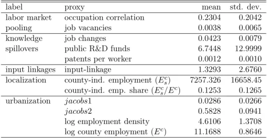
As argued above, despite having the same label ’knowledge spillovers’ the mechanism between job changes and the patents / R&D funds variables is distinct. For this reason these proxies are unlikely to be collinear and I will use them simultaneously in regressions. The correlation coefficients between the agglomeration mechanism variables and between the industrial environment variables shown in the Appendix in tables C.1 and C.2, respec-tively, confirm this. Table 1 presents summary statistics for all the agglomeration variables described above.

Table 1: summary statistics of agglomeration variables

label proxy mean std. dev.

labor market occupation correlation 0.2304 0.2042

pooling job vacancies 0.0038 0.0065

knowledge job changes 0.0423 0.0079

spillovers public R&D funds 6.7448 12.9999

patents per worker 0.0012 0.0010

input linkages input-linkage 1.3293 2.6760

localization county-ind. employment (E_sc) 7257.326 16658.45 county-ind. emp. share (Ec

s/Ec) 0.1253 0.1265

urbanization jacobs1 0.0286 0.0266

jacobs2 0.5828 0.0941

log employment density 4.6106 1.3708

log county employment (Ec) 11.1688 0.8646

Notes: The number of observations is 18569 for all variables.

Concerning endogeneity of these agglomeration variables, I am more confident with the job changes than with the other two spillover measures. It might be the case that the number of patent applications are correlated with productivity, simply because high productivity plants hire a more innovative personnel than low productivity plants. Alike, high productivity plants might be more successful in acquiring public funds than their competitors. Then these measures would just indicate, where high productivity plants are located, but would not imply the presence of knowledge spillovers. With regard to input linkages and labor market pooling I am carefully optimistic that endogeneity does not drive the results here. Firstly, because reasoning like above appears implausible in these cases. Secondly, Ellison et al. (2010) use a sophisticated set of instruments for similar agglomeration proxies and find their initial OLS results to be fairly stable. Similarly, even instrumenting employment density in Ciccone and Hall (1996) or in Combeset al. (2010) reinforced its prior OLS coefficients.

4

Results

4.1 Production functions results

Table 2 reports the results from the estimation of production functions under four speci-fications. The first column contains the result from a simple OLS regression of equation (1). The coefficients in the second column have been produced, applying only the OP estimation algorithm as described in section 2.2. The third and fourth column result from the KG procedure in equation (4). Finally the fifth and sixth column refer to the com-bined OP/KG adjustment from equation (A.4) and (A.8), the preferred specification. In both estimations where unobserved output prices are substituted, adjusted and unadjusted coefficients are reported. In the two cases, where the selection bias has been taken care of, all variables capturing agglomeration mechanisms (subsumed in the parameter Gc_t in the above equations) have been used as predictors in the Probit model. Controls for the share of high skilled workers, a west-dummy and industry fixed effects are included in all production functions20.

Table 2: basic production function coefficients

OLS OP KG OP/KG e α α_e α_e α α_e α materials 0.6522 0.6484 0.6512 0.8230 0.6474 0.8049 (0.0063) (0.0043) (0.0063) (0.0043) labor 0.3300 0.3287 0.3312 0.4186 0.3297 0.4100 (0.0086) (0.0057) (0.0087) (0.0057) capital 0.0472 0.0465 0.0472 0.0596 0.0458 0.0569 (0.0037) (0.0006) (0.0035) (0.0006) demand ela. - - 5.58 5.84 (1.1797) (1.6137) west 0.1212 0.1012 0.1204 0.1522 0.1007 0.1272 (0.0090) (0.0090) (0.0090) (0.0061) high-skilled share 0.1508 0.1465 0.1481 0.1872 0.1434 0.1783 (0.0178) (0.0159) (0.0177) (0.0161) N 18569 18569 18569 18569 R2 0.9711 - 0.9711

-Notes: Cluster robust standard errors at the plant level are given in parenthesis. In the OP and OP/KG case the standard errors were obtained by bootstrapping. Coefficients for the industry fixed effects are omitted.

Throughout table 2, all coefficients have the expected magnitude and are highly sig-nificant. Beginning in column 1, scale elasticities of labor, capital and intermediate inputs sum to 1.03, hence this production function exhibits increasing returns to scale. A sim-ple Wald test confirms that the sum α_ek+αel+αem is significantly different from unity.

20

Adding more controls like a workers’ council dummy and the legal form left the results in the following analysis unchanged. However, if those variables are themselves outcomes of the plant’s TFP rather than determinants, the production function estimation is distorted. Because those variables are nor decisive nor part of the research question, I opted for leaving them out.

The distinction between the first and the second column is, that I have accounted for the positive correlation between inputs and productivity. Just as predicted by theory, we see lower scale elasticities for capital, labor and materials, but still the sum of these coefficients indicate the presence of increasing returns to scale.

In estimating the production function according to Klette and Griliches (1996), I found that the year-industry specific term(rs_It−ps_It) did not exhibit enough temporal variation to identify industry specific demand elasticities in the presence of industry fixed effects. For this reason, I opted to keep the industry fixed effects and constrain the demand elas-ticity to be equal in all industries. In the KG case this elaselas-ticity across all industries is estimated to 5.58. Recall that through the combination of production and demand side, the original coefficients are reduced form parameters. After rescaling by _σσ₋₁ (in column 4) all scale estimates are higher than in the prior models and the production function exhibits substantial returns to scale.

Combining this KG specification with the OP procedure, again I find lower scale esti-mates due to the correction of the transmission bias. Here, the demand elasticity is 5.84. I have also estimated the same equation with industry specific demand elasticities and find their range to be quite narrow21. The highest demand elasticities are in ’wholesale and retail trade’ (6.84), in ’food, beverages and tobacco’ (6.54) and in ’transport, storage and communication’ (6.43). The industries least sensitive to price differences are ’wood products’ (5.41), ’other transport equipment’ (5.43) and ’precision and optical instruments’ (5.50). The latter industries tend to produce less standardized products than the three industries with the highest demand elasticities, so this finding accords with our intuition. To wrap up, all estimated parameters are quite plausible. Scale estimates are positive, significant and sum to somewhat more than unity. Also as expected, the west-dummy is highly significant and indicates that establishments in West Germany generate around 12% higher revenues with the same amount of inputs. Considering that demand elasticities are estimated at the plant level, their range from 5.4 to 6.8 seems reasonable, too. These numbers conform to the findings of other studies, e.g. De Loecker (2011). The author even had segment specific physical output quantities available and finds demand elasticities for subsectors of the textile industry between 2.8 and 6.2 in a similar setting. Also based on a CES utility function, Hanson (2005) estimates market potential functions from county specific data for the US. He obtains demand elasticities in a range of 5 to 7.5.

4.2 Agglomeration mechanisms results

Table 3 presents results from regressing each of the six proxies for agglomeration mecha-nisms separately on each of the four basic TFP measures, obtained from the production functions described in the previous subsection. All estimations control for year and in-dustry fixed effects. In addition, all agglomeration variables are standardized to have a zero mean and a standard deviation of one, in order to provide direct comparability of

21

Results are not reported, but are available upon request. These results were estimated from an equation without industry fixed effects.

their relative impact. Here and in the following regressions standard-errors are clustered at the county-industry-year level to account for a possible intra-group correlation of plant’s error components. Otherwise, standard errors are biased downwards in regressions with micro-level data and aggregated regressors (Moulton 1986). All variables have a positive coefficient and are comparable in size across the different TFP measures. Regarding the strength of the proxies, R&D and the occupational correlation rank on top in all ver-sions. Meaningful differences in the significance level across columns 1-4 emerge only in the patent variable. Besides it is the only variable lacking statistical significance at the 5% level. Before going deeper into interpretations, we want to inspect multivariate regressions, because as argued above, they will provide us with more reliable insights about the relative importance and magnitude of microeconomic agglomeration channels.

Table 3: agglomeration mechanisms in univariate regressions

OLS OP KG OP/KG occ-cor 0.0150 0.0206 0.0178 0.0246 (0.0000) (0.0000) (0.0000) (0.0000) R2 0.0018 0.0038 0.0042 0.0063 vacancies 0.0084 0.0098 0.0104 0.0119 (0.0068) (0.0017) (0.0058) (0.0015) R2 0.0012 0.0023 0.0037 0.0048 job-changes 0.0131 0.0135 0.0163 0.0166 (0.0000) (0.0000) (0.0000) (0.0000) R2 0.0019 0.0029 0.0044 0.0055 patents 0.0057 0.0108 0.0070 0.0132 (0.0566) (0.0003) (0.0569) (0.0003) R2 0.0009 0.0025 0.0033 0.0050 R&D 0.0163 0.0185 0.0200 0.0225 (0.0000) (0.0000) (0.0000) (0.0000) R2 0.0027 0.0042 0.0052 0.0067 input-linkage 0.0066 0.0061 0.0084 0.0075 (0.0014) (0.0029) (0.0009) (0.0025) R2 _{0.0009 0.0018 0.0034 0.0043}

Notes: p-values in parentheses are computed with cluster-robust standard errors at the county-industry-year level. Year and in-dustry fixed effects are included in all estimations. Each is based on 18569 observations. Covariates are standardized to have a zero mean and a standard deviation of one.

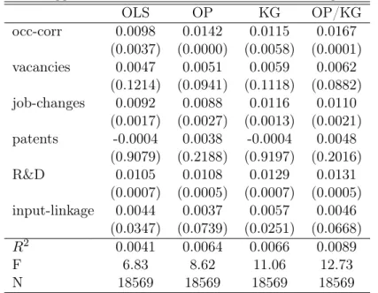
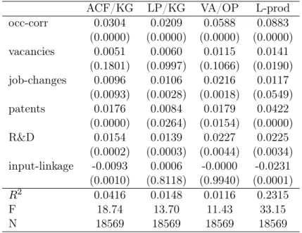
Table 4 contains the results from regressions of the basic TFP measures against all six agglomeration variables. Under the preferred specification (column 4), the labor market pooling measure and two of the knowledge spillovers are still positive and significant. More precisely, the number of job changes and the amount of funds for research projects posi-tively affect the average productivity of plants in a county, though the relative impact of R&D spillovers is slightly higher. The interpretation of this coefficient is that an increase by one standard deviation (13 MillionAC p.a.) would raise the average TFP in that county by 1.3 percentage points. However, plants benefit considerably more from a local labor

market with an occupational structure similar to their own industry. If the endogeneity bias and the omitted price bias are not accounted for, the magnitude of these positive effects is underestimated. In fact the TFP measure from the OLS regression yields 20-42% lower coefficients. Simple OLS and the KG regressions would even suggest that these three significant mechanisms are of the same importance. Furthermore, table 4 reveals that patent applications, input linkages and job vacancies in a county are not major sources of agglomeration externalities, or at least the way these variables are constructed does not capture the underlying mechanism well. This might especially be true for the input linkage proxy, whose construction could have been improved with information about local or even plant specific input-output flows. Concerning the considerable differences in the perfor-mance of the patent proxy in multivariate and univariate regressions it might be possible that its significance in the univariate regression is caused by positive correlation with some of the other agglomeration proxies. However, the correlation coefficients among the ag-glomeration variables displayed in table C.1 in the Appendix are all below 0.3 and variance inflation factors show, that the these regressions do not suffer from multicollinearity.

Greenstone et al.(2010) reach a similar conclusion across their univariate regressions (even though from somewhat different agglomeration proxies): labor market pooling gener-ates relatively higher productivity effects than knowledge spillovers and supplier proximity has no measurable effects. The evidence on co-agglomeration between industries in Ellison

et al.(2010) is not quite in line with table 3. In essence, the authors find positive effects for all three Marshallian forces with input-output relations being the most important followed by labor pooling22_.

A direct comparison between the OP and the OP/KG is especially insightful. In the OP case, the TFP estimate contains price variation. That is, because unobserved plant level prices have not been accounted for, they are included in the residual term. So instead of regressing true TFP against the agglomeration variables, the estimating equation in fact looks like this

ωjt+pjt=β0+Gct+ejt

Under this OP specification, we observe lower coefficients in table 4 for each of the six agglomeration mechanisms subsumed inGc_t. Hence unobserved plant level prices are neg-atively correlated with Gc_t. On the one hand, this suggests that plants quote on average lower prices in counties characterized by (1) having a similar occupational structure to their own industry, (2) high public R&D funding and (3) a high labor turnover. Because these characteristics are also associated with higher plant TFP, this finding, on the other hand, is in line with the prediction that high productivity plants quote lower prices (Melitz 2003). The same interpretation holds from a comparison between the results of the OLS and the KG productivity estimate in table 4. Likewise, the former TFP measure incorporates price variation while the latter does not.

22

The different outcome here is puzzling because the construction of the input relations variable is quite similar in Ellisonet al.(2010) and in Rigby and Essletzbichler (2002), as mentioned in footnote 15.

Table 4: agglomeration mechanisms in multivariate regressions OLS OP KG OP/KG occ-corr 0.0098 0.0142 0.0115 0.0167 (0.0037) (0.0000) (0.0058) (0.0001) vacancies 0.0047 0.0051 0.0059 0.0062 (0.1214) (0.0941) (0.1118) (0.0882) job-changes 0.0092 0.0088 0.0116 0.0110 (0.0017) (0.0027) (0.0013) (0.0021) patents -0.0004 0.0038 -0.0004 0.0048 (0.9079) (0.2188) (0.9197) (0.2016) R&D 0.0105 0.0108 0.0129 0.0131 (0.0007) (0.0005) (0.0007) (0.0005) input-linkage 0.0044 0.0037 0.0057 0.0046 (0.0347) (0.0739) (0.0251) (0.0668) R2 0.0041 0.0064 0.0066 0.0089 F 6.83 8.62 11.06 12.73 N 18569 18569 18569 18569

Notes: p-values in parentheses are computed with cluster-robust standard errors at the county-industry-year level. Year and in-dustry fixed effects are included in all estimations. Covariates are standardized to have a zero mean and a standard deviation of one.

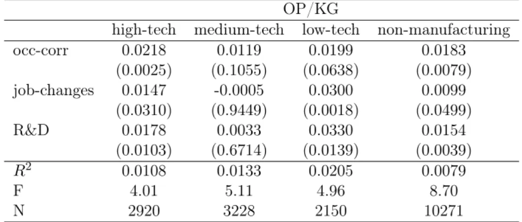
Another interesting question is, whether these agglomeration mechanisms differ be-tween industries. Due to the demanding data requirements of this investigation, the number of observations is quite low in some of the 22 industries. Therefore, I combined industries according to their R&D intensity into four groups (compare table B.1). Table 5 contains the results from the regression of those agglomeration proxies, which exhibited a significant coefficient in the multivariate regressions, against the OP/KG productivity. High-tech in-dustries exhibit a strong positive correlation between TFP and all agglomeration proxies. The magnitude of their impact is generally higher than in the pooled industry case but their ranking is preserved. The same is true for plants from non-manufacturing industries. In medium-tech sectors (column 2), no significant influence is found for either of the vari-ables. For low-tech industries a higher labor turnover and R&D funding to companies in their county are associated with a higher productivity level. Altogether it seems there are sectoral differences, but plants across the most R&D intensive sectors, non-manufacturing industries and even low-tech sectors benefit from labor market pooling and knowledge spillovers.

4.3 Urbanization and localization results

Table 6 displays the results from multivariate regressions using the industrial environment proxies. All covariates except for county size (Ec_{) are standardized to have a zero mean}

and a standard deviation of one. Across the four basic TFP measures the emerging picture is quite uniform. There is no sign that the industrial diversity is positively correlated with

Table 5: agglomeration mechanisms for industry groups OP/KG

high-tech medium-tech low-tech non-manufacturing

occ-corr 0.0218 0.0119 0.0199 0.0183 (0.0025) (0.1055) (0.0638) (0.0079) job-changes 0.0147 -0.0005 0.0300 0.0099 (0.0310) (0.9449) (0.0018) (0.0499) R&D 0.0178 0.0033 0.0330 0.0154 (0.0103) (0.6714) (0.0139) (0.0039) R2 0.0108 0.0133 0.0205 0.0079 F 4.01 5.11 4.96 8.70 N 2920 3228 2150 10271

Notes: p-values in parentheses are computed with cluster-robust standard errors at the county-industry-year level. Year and industry fixed effects are included in all estimations. Covariates are standardized to have a zero mean and a standard deviation of one. The dependent variable is plant level TFP from the OP/KG model.

plant level TFP. Recall that for both diversity measures the theory of Jane Jacobs predicted a negative coefficient. In contrast, we see that the share of the three largest industries in a county (jacobs2) exerts apositive and significant effect on productivity. Alongside, only county size shows significant coefficients in columns 1 to 623. Also standardizing this variable, for example in column 4, leads to a coefficient of 0.0163. Hence the share of the three largest industries is relatively more important. Remarkably, the two significant proxies again grow in magnitude, when the transmission bias and the omitted price bias are accounted for.

These multivariate regression also reveal that the share of the three largest industries dominates the effect of the share and size in plant’s own industry. In univariate regressions each of these three proxies shows a positive and significant influence on the OP or OP/KG TFP measure. To check whether multicollinearity is an issue here, some covariates are dropped in columns 5 and 6. Without the industrial diversity index all coefficients remain relatively unchanged. In column 6 the dominant variablejacobs2was excluded, leading to a much higher and more significant coefficient of the own industry employment share. These tests underline the robustness of the results, because they leave the previous conclusions unchanged: (1) A 10% increase in the size of a county is associated with a 0.2% to 0.3% higher plant level productivity. (2) The industrial specialization, either captured through the employment share of the own industry or the three largest industries in a county has a positive influence, whereas no significant effect is found for industrial diversity.

23_{The density of a county is not included in these regressions, because it is highly correlated with county} size. However, when I replaced county size with the density variable, qualitatively similar results were obtained.

Table 6: TFP against urbanization and localization variables

OLS OP KG OP/KG OP/KG OP/KG

Ec 0.0124 0.0158 0.0149 0.0189 0.0175 0.0288 (0.0025) (0.0001) (0.0030) (0.0001) (0.0003) (0.0000) Ec i 0.0029 0.0030 0.0042 0.0042 0.0044 0.0018 (0.3835) (0.3660) (0.3187) (0.3002) (0.2762) (0.6673) E_sc/Ec -0.0049 0.0010 -0.0084 -0.0003 0.0002 0.0177 (0.4132) (0.8738) (0.2519) (0.9645) (0.9806) (0.0098) jacobs2 0.0213 0.0230 0.0262 0.0279 0.0293 -(0.0000) (0.0000) (0.0000) (0.0000) (0.0000) jacobs1 0.0027 0.0034 0.0035 0.0043 - -(0.4446) (0.3433) (0.4275) (0.3263) R2 0.0064 0.0093 0.0089 0.0118 0.0117 0.0081 F 11.22 14.50 16.12 19.37 21.51 15.87 N 18569 18569 18569 18569 18569 18569

Notes: p-values in parentheses are computed with cluster-robust standard errors at the county-industry-year level. Year and industry fixed effects are included in all estimations. Except for county size, all covariates are standardized to have a zero mean and a standard deviation of one.

5

Robustness checks

The following section presents variations in the range of industries, changes in the spatial level of aggregation, additional controls for the type of county a plant resides and finally results of different TFP estimation methods. It turns out that the key insights presented so far are fairly robust to these variations.

5.1 Manufacturing only

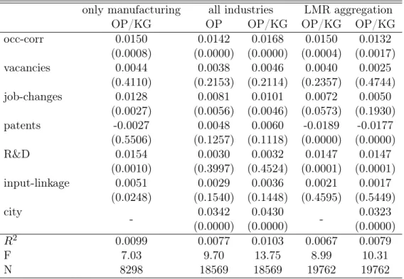
In order to verify that the results are not driven by the non-manufacturing industries, the same analysis is conducted without them. Both the estimation of the production function and the investigations on agglomeration economies are found to be largely unchanged. I interpret this as a sign that the concept of production functions should not be limited to the manufacturing sector, and that agglomeration forces spread over a wide industrial range. The only exception seems to be supplier linkages. This mechanism is now significant though still much smaller than labor market pooling and knowledge spillovers. Using the preferred OP/KG TFP as a showcase, the first column in table 7 and 8 contains the results for agglomeration mechanisms and industrial environment variables, respectively.

5.2 Control for city-counties

As a second robustness check, additional controls for the nature of the county are included. In Germany some counties are made up just of one large city, others are sparsely populated but vast in space. For instance, because it is less likely for large cities than for rural areas to reach a certain degree of specialization, it might be inappropriate to pool all county

Table 7: agglomeration mechanisms - robustness checks

only manufacturing all industries LMR aggregation

OP/KG OP OP/KG OP/KG OP/KG

occ-corr 0.0150 0.0142 0.0168 0.0150 0.0132 (0.0008) (0.0000) (0.0000) (0.0004) (0.0017) vacancies 0.0044 0.0038 0.0046 0.0040 0.0025 (0.4110) (0.2153) (0.2114) (0.2357) (0.4744) job-changes 0.0128 0.0081 0.0101 0.0072 0.0050 (0.0027) (0.0056) (0.0046) (0.0573) (0.1930) patents -0.0027 0.0048 0.0060 -0.0189 -0.0177 (0.5506) (0.1257) (0.1118) (0.0000) (0.0000) R&D 0.0154 0.0030 0.0032 0.0147 0.0147 (0.0010) (0.3997) (0.4524) (0.0001) (0.0001) input-linkage 0.0051 0.0029 0.0036 0.0021 0.0017 (0.0248) (0.1540) (0.1448) (0.4595) (0.5449) city - 0.0342 0.0430 - 0.0323 (0.0000) (0.0000) (0.0000) R2 0.0099 0.0077 0.0103 0.0067 0.0079 F 7.03 9.70 13.75 8.99 10.31 N 8298 18569 18569 19762 19762

Notes: p-values in parentheses are computed by the use of cluster-robust standard errors. Year and industry fixed effects are included in all estimations. Agglomeration variables are standardized to have a zero mean and a standard deviation of one. In column five and six all covariates but the city-county dummy are LMR and time specific.

types24. A dummy which indicates whether the county is a large city or not is added to the estimation of agglomeration economies25.

In table 7 the most remarkable consequence of this extension is that the R&D variable loses its significance. R&D funding exhibits by far the highest correlation (0.72) with county size (cf. table C.1). It is difficult to judge whether the assumed spillover itself is spurious, or whether the county control just outrivals its effect. An argument in favor of the second interpretation is that the induced insignificance of R&D does not always occur, as we will see in the following extension. Apart from that change the prior findings still hold. Labor market pooling and knowledge spillovers positively impact on plant’s TFP. As before, their strength and significance rises if OP/KG adjusted productivity instead of price biased TFP is examined. The same applies to the urbanization and localization variables displayed in table 8. County size and the share of the three largest industries in a county (jacobs2) boost productivity. Accordingly, this insight is robust to the control of city-counties as well as to the omission of non-manufacturing industries.

24

I thank Georg Hirthe for bringing this issue up. 25

I also experimented with nine different county type dummies classified according to the size and density of a region. However, all results were very similar to those with just the city dummy.

Table 8: urbanization and localization - robustness checks only manufacturing all industries LMR aggregation

OP/KG OP OP/KG OP/KG OP/KG

Ec 0.0222 0.0153 0.0180 0.0018 0.0000 (0.0010) (0.0002) (0.0004) (0.6838) (0.9912) Ec_i 0.0287 0.0029 0.0040 -0.0006 -0.0009 (0.3089) (0.3840) (0.3225) (0.9265) (0.9007) Ec_s/Ec -0.0213 0.0010 -0.0002 0.0084 0.0076 (0.0715) (0.8655) (0.9767) (0.3756) (0.4247) jacobs2 0.0249 0.0220 0.0262 0.0206 0.0179 (0.0000) (0.0000) (0.0000) (0.0000) (0.0000) jacobs1 0.0035 0.0035 0.0044 -0.0085 -0.0075 (0.5150) (0.3338) (0.3129) (0.0176) (0.0367) city - 0.0042 0.0072 - 0.0284 (0.5877) (0.4381) (0.0001) R2 _{0.0138 0.0093 0.0118 0.0065 0.0074} F 10.70 13.17 17.60 9.24 9.68 N 8298 18569 18569 19762 19762

Notes: p-values in parentheses are computed by the use of cluster-robust standard errors. Year and industry fixed effects are included in all estimations. Except for county size, all agglomeration covariates are standardized to have a zero mean and a standard deviation of one. In column five and six all covariates but the city-county dummy are LMR and time specific.

5.3 Aggregation to labor market regions

Another interesting exercise is to vary the boundaries of the spatial units and retest for agglomeration economies. Drawing this analogy examines the externalities’ scope. Be-cause gains from agglomeration reside in the proximity of agents, it is natural to presume that lower agglomeration externalities are observed in larger spatial entities. Furthermore, this extension evaluates the sensitivity of the results to the modifiable areal unit problem. Eckeyet al.(2006) propose a delineation of one or several counties to labor market regions (LMR) which cover the entire German territory. The delineation is based on a factor anal-ysis of commuting patterns between counties, subject to two restrictions: the LMR has a population of at least 50.000 and commuting time must not exceed 60 minutes26_{. Due to}

the labor market related division, it is reasonable to expect the labor market externality to decline less than knowledge spillovers. In order to implement the robustness check, all ag-glomeration variables are reconstructed on the level of LMRs and the OP/KG production function is estimated again, containing LMR specific variablesGlmr. Production function coefficients are very similar to the county case and are omitted for brevity. Columns 4 and 5 in table 7 present the corresponding multivariate regressions with and without the city dummy, respectively. Though being significant it has a negligible impact on the other covariates. In columns 4 and 5 the correlation between one LMR-industry and the rest of the LMR as well as the amount of public R&D funding per LMR raise plant’s TFP.

How-26

ever, the knowledge spillover transmitted via job changes is now insignificant. While the R&D related spillover seems to be unaffected by the greater distance, the influences from occupational correlation and job changes are now less significant and smaller in size, as one would have expected. This points to the conclusion, that a finer county level is more appro-priate for the investigation of agglomeration economies. For the record: The modification of spatial units does not alter the agglomeration economies fundamentally. In the three robustness checks up to here, labor market pooling and at least one knowledge spillover still have been detected. Moreover, agglomeration economies are again underestimated without the OP/KG adjustment (not reported due to space constraints).

Surprisingly, the patent variable has a negative and highly significant coefficient in both LMR estimations of table 7, thus more patent applications seem to drag down productivity. At first sight, this is contrary to the predictions in the regional science literature. However, patents also have a strategic value which is unrelated to the actual value of the invention. Firms increasingly use patents as offensive or defensive instruments in negotiations and trials (cf. Hall and Ziedonis (2001), Hu and Jefferson (2009)). Another aspect of this "patent paradox" is that "patents are not an indicator of research productivity, or that the number of patents per R&D expenditure would not indicate differences in innovation performances" (de Rassenfosse and van Pottelsberghe 2009: 779). In so far as profuse patenting for strategic competition takes up resources, the negative correlation with TFP is economically meaningful. A reason why the negative sign has not surfaced before, lies in the construction of the variable. The data at use is patent applications at the residence county of the applicant(s). Now that an LMR aggregates counties according to commuter flows, the discrepancy between patent counts at the workplace and at the inventors residence diminished. The actual connection between the patent counts and the plant is more forthright. What intuitively appeared to be a measure innovativeness turned out to abate productivity.

Columns 4 and 5 in table 8 report the results from regressing the urbanization and localization variables on OP/KG TFP. The specialization variable (jacobs2) again is highly significant. In contrast to prior estimations the employment size of a labor market region has no effect on TFP. Even though the commuting time within an LMR does not exceed one hour, this suggests that proximity is important on a rather small scale. Controlling whether a plant resides in a city or not, does not alter the results. Yet, the dummy is significant and indicates that TFP is on average almost 3% higher in city-counties. Note also that industrial diversity (jacobs1) now can not be rejected at the 5% significance level and its coefficient is negative as expected. This conforms to the observation in Beaudry and Schiffauerova (2009) in that it is more likely to detect Jacobs externalities, the larger the level of geographical aggregation.

5.4 Alternative TFP estimations

In this subsection I discuss results from four different specifications of the original OP framework: (1) the Levinsohn and Petrin (2003) estimation approach, which relies on a different control function than Olley and Pakes (1996), (2) the Ackerberget al. (2006) correction for the OP procedure, (3) taking value added instead of revenue based production functions, (4) using labor productivity instead of estimated TFP to identify agglomeration economies;

Levinsohn and Petrin (2003) (LP, henceforth) modify the OP estimation and use inter-mediate input demandmjt =m0t(kjt, ωjt(Gct))instead of investment demand to control for

unobserved productivity27. Before we assumed that productivity is the only unobserved factor in the investment demand and that the function is monotonic in productivity. Ob-viously, in the LP framework we have to make these two assumptions with respect to the intermediate inputs demand mjt. Observing considerable different results from both

models would lead to the conclusion, that one of control functions is defective. The lower panel of figure A.1 in the Appendix provides a graphical assessment of the invertability assumption. Intermediate input demand is increasing much sharper in productivity, but also decreasing earlier and faster than in the upper OP/KG case for any possible value of K. This suggests that the required invertability condition is more likely to hold for the investment control function. For the details on the implementation of the LP and the following Ackerberget al.(2006) estimation the reader is referred to the Appendix A.2 and A.3, respectively.

Ackerberg et al. (2006) (henceforth ACF) criticize the identification of coefficients on variable inputs in the Olley and Pakes (1996) and the Levinsohn and Petrin (2003) ap-proach. The authors consider that L and M are not chosen independently, but rather might be functions in kjt and ωjt, just like plant’s investments are. Substituting by

ωjt=ht(kjt, ijt, Gct) yields

ljt =lt(ωjt, kjt) =lt0(kjt, ijt, Gct) and (5)

mjt =mt(ωjt, kjt) =m0t(kjt, ijt, Gct) (6)

Plugging these functions into the production function (A.4), reveals that both equation (5) and (6) are perfectly collinear with the termφt(kjt, ijt, Gct), thus preventing the

identifica-tion of αl and αm in the first stage. Building on the proposal in Ackerberg et al. (2006)

the modified estimation algorithm relies on a different timing assumption of input choices. Taking value added (VA) instead of revenue production functions can be seen as another response to the collinearity problem brought up by Ackerberget al.(2006). Of course, value added production functions sidestep part of the problem, because the perfectly variable

27_{Their modification was primarily developed for datasets in which a large number of firms report} missing or zero investments. In the present case the sample size would not be increased much, because the construction of the capital variable already relies on plants’ investments. For better comparability of results the LP estimation is based on the preceding sample.

inputM does not have to be identified at all. Instead of changing the assumptions on the timing of input choices, according to Bond and Söderbom (2005) identification of perfectly variable inputs can be achieved, if the input factor encounters adjustment costs. That is also a maintainable assumption in the case of labor. Thus, either of the OP, LP or KG estimation algorithms can be performed analogous to the revenue case. Due to space constraints just the simple OP adjustment is presented. Nevertheless, this does not imply that value added is the superior measurement of production, cf. the discussion in Basu and Fernald (1997). At last, the following tables also contain regressions with log labor productivity as dependent variable, being computed as log revenues minus log labor input. The purpose of this exercise is to ascertain, whether a measure, which is not estimated from a production function, leads to the same inference as TFP measures.

5.4.1 Results for the additional TFP measures

Coefficients from the combined LP/KG and ACF/KG production functions are close to those obtained from OP/KG model in table 2. The largest deviation is given in the ACF capital coefficient which is reduced by more than 50%, casting some doubt on the accuracy of the procedure. This finding is unexpected, because the capital coefficient has already been identified in the second stage in the prior OP estimations. Having very similar coefficients in the LP/KG production function suggests that the identification of perfectly variable inputs (mjt), was not inaccurate before28.

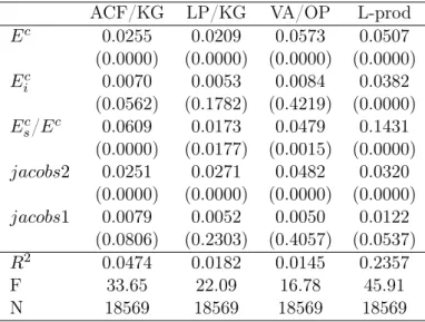
Of more importance is the question, if these productivity estimates lead to different con-clusions regarding agglomeration economies? The following tables 9 and 10 display results from multivariate regressions with one of the four additional TFP measures as dependent variable and agglomeration mechanisms and industrial environment proxies, respectively, as covariates. Table 9 confirms that occupational correlation exerts the largest influence on whichever TFP measure. For the ACF, VA and LP productivity job changes and R&D funding also show a positive and significant coefficient. In sum across all productivity measures, 21 out of 24 coefficients confirm that a labor market pooling measure exerts the largest impact on plant’s performance followed by R&D funding and job turnover, two knowledge spillover proxies29_.

Taking a closer look, we see that results from the LP productivity are very similar to the preferred OP/KG estimation. Column 3 reminds us that results from revenue and value added production functions are not comparablequantitatively. The value added TFP implies that a one standard deviation increase in public R&D expenditure for innovative projects would lead to a productivity increase of 2.2%, whereas inference from a revenue based productivity measure implies a 1.4% increase. Apart from the quantitative diver-gence the main conclusions from the OP/KG model remain valid. So it seems that whether intermediate inputs are identified in the first or second stage or not at all, is not crucial for

28_{De Loecker (2011) made the same observation in his dataset.} 29

Another piece of evidence is that across all eight productivity measures presented so far the variables with the highestR2 _{in univariate regressions are the occupational correlation and R&D funding.}