An improved saliency detection algorithm based on Itti’s model

(1)

ISSN 1330-3651(Print), ISSN1848-6339 (Online) UDC/UDK 004.81:159.937.5.952.1

AN IMPROVED SALIENCY DETECTION ALGORITHM BASED ON ITTI’S MODEL

Zhongshan Chen, Yan Tu, Lili Wang

Original scientific paper Visual attention mechanism (VAM) automatically ignores the superfluous information and pays attention to the most significant objects when people are watching the pictures. There are numerous bottom-up visual attention computational models to detect the salient area of an image. In this paper, an improved visual attention computational model based on Itti’s model is proposed, which is comprised of three components. Firstly, the lower-level primitive image features s are extracted from CIELa*b* color space instead of RGB color space; secondly, the feature images are decomposed into wavelet pyramids by wavelet-based multi-scale transform. Thirdly, a new strategy is used to combine all conspicuity maps into a final saliency map with different weights, which are proportional to the contribution of each conspicuity map. Compared with Itti’s models, subjective experiments prove that the approach proposed in this paper is more effective.

Keywords: bottom-up model, image feature, saliency map, visual attention mechanism (VAM) Poboljšani algoritam otkrivanja istaknutih elemenata zasnovan na Itti modelu

Izvorni znanstveni članak Kad ljudi promatraju slike, mehanizam vizualne pažnje (VAM) automatski zanemaruje nepotrebnu informaciju i pažnju usmjerava na najvažnije predmete. Postoje brojni računalni modeli za otkrivanje najistaknutijeg područja slike usmjeravanjem pažnje od dna slike prema gore. U ovom se radu predlaže poboljšani računalni model vizualne pažnje zasnovan na Itti modelu, a sastoji se od tri komponente. Najprije se s značajke nižeg nivoa osnovne slike izdvajaju iz područja boje CIELa*b* umjesto područja boje RGB; poslije toga se značajke slike rastavljaju u valićaste piramide pomoću valićaste osnove višeskalne pretvorbe. Kao treće, primjenjuje se nova strategija za sastavljanje svih upadljivih linija u završnu mapu istaknutih elemenata s različitim težinama, koje su proporcionalne doprinosu svake pojedinačne istaknute karakteristike. U usporedbi s Itti modelom, exsperimenti dokazuju da je pristup predložen u ovome radu učinkovitiji.

Ključne riječi: mapa istaknutih elemenata, mehanizam vizualne pažnje (VAM), model odozdo prema gore, značajka slike 1 Introduction

With the rapid development of multimedia information and Internet technology, images are increasingly become the essential carrier of spreading information. Selective VAM is one of the most crucial mechanisms of the human visual system (HVS), which can effectively eliminate the interference of redundant visual information and focus on the interested region when observing an image. It significantly reduces the complexity of the information processing and improves the processing speed.

Many visual attention computational algorithms were proposed to simulate what is likely to attract the attention of observers. There are two different VAM: bottom-up and top-down [1, 7, 11, 17]. The bottom-up visual attention is a data-driven process, human selectively focus on salient parts according to a variety of early visual features of the input image because of the primitive selective attention. The top-down visual attention is a directed task-driven process, human pays attention on the elements which is similar to the observer's goal. The prior knowledge [12, 13, 16] influences the recognition ability in top-down processing. It is generally considered that the top-down process is based on the bottom-up process.

1.1 Previous computational models

During the past several decades, many algorithms of bottom-up visual attention have been proposed [2 ÷ 6, 8, 10, 14 ÷ 16], which are generally divided into four categories [3, 4]:

1) Space-based model: The classical model is Itti’s model. Itti et al. devised a visual attention model based on

the behaviour and neuronal architecture of the primates’ early visual system in 1998 [10]. Recently, Valenti et al. submitted a saliency detection model by calculating the centre-surround differences of edges, colour, and shape of images [16].

2) Frequency-based model: The classical model is SR model. Hou et al. devised a saliency detection model based on a concept defined as spectral residual (SR) in 2007 [8]. Guo et al. discard the amplitude spectrum and utilize the original phase spectrum of the image to design a phase-based saliency detection model (FQFT) [5] by inverse Fourier transform (IFT).

3) Object-based model: According to schema theory, the unit of selective visual attention is perceptual object created by Gestalt rules. Bruce et al. described visual attention based on the principle of maximizing information [2]. Liu et al. used the technology of machine learning to obtain the saliency map of images [14].

4) Graph-based model: According to schema theory, selective visual attention selects different features of object. The classical model is GBVS model. A graph-based visual saliency (GBVS) model was proposed by Harel et al. The model used a better dissimilarity measure for saliency than Itti’s model [6]. Later, a saliency detection model based on the colour and orientation distributions in images was designed by Gopalakrishnan et al. [4].

1.2 The motivation of this paper

Itti’s model is generally thought to be a classic one in models mentioned above, which is widely used to detect the salient area for some given scene.

(2)

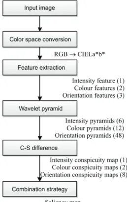
characteristics such as the intensity, colour opponency and orientation, Itti’s model uses these features as the primitive information. In data pre-treatment phase, the features are represented in a series of multilayer Gaussian pyramids after linear filtering. Then three conspicuity maps corresponding to three visual features are separately obtained by calculating the centre-surround differences of [10]. The final saliency map is achieved by the mean value of three conspicuity maps, as shown in Fig. 1.

Figure 1 Itti's model

Itti’s model is now widely recognized and applied in the fields of computer vision, such as object recognition, image compression and coding. However, there still are some shortcomings of Itti’s model. Firstly, it does not take into account different resolution of original images. That is, for all of the input images, Gaussian pyramid obtained by Itti’s model has the same structure with 9 layers. The size of saliency map is only 1/256 of the original image; secondly, Itti’s saliency map calculated by the multi-scale center-surround differences cannot reflect the whole significant area but the exact location of the significant point; thirdly, it is not easy to determine the size and shape of significant area. The shape of significant area by Itti’s model is a circular region with a fixed radius regardless of different size of attention area, which sometimes may contain too many background regions and ignore the integrity of the interesting target.

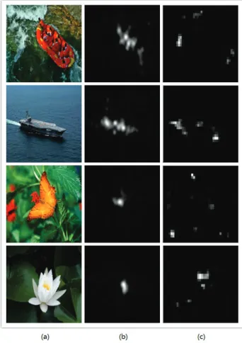
In most cases, the saliency map gotten from Itti’s model is not accurate enough because of these shortcomings, as shown in Fig. 2. It is clear that the saliency maps from Itti’s model contain some error points out of salient area and the results are also incomplete for salient object, which is different from eye tracking recording at the second column.

Figure 2 Performance comparison: (a) Original images. (b) Saliency maps from eye tracking. (c) Saliency maps from Itti’s model The purpose of this study is to improve Itti's model further and obtain a more accurate saliency map. Our improved model focuses on the bottom-up approach. This paper is arranged as follows. In Section 2, the improved algorithm is elucidated in detail. In Section 3, the results of the improved model and Itti's model are compared with the eye tracking experimental results. Finally, the paper draws the conclusions by summarizing our work.

2 The improved visual attention model

In this paper, the proposed model is more in accord with the human vision system. The overall work flow of the new model is depicted in Fig. 3.

The improved model includes the following four modules. Firstly, extract the early visual features from the CIELa*b* colour space. Secondly, establish the wavelet pyramids. Thirdly, calculate the centre-surround differences to simulate the function of human visual receptive fields. Lastly, obtain the final saliency map by combining all conspicuity maps with different weights proportional to the saliency of each conspicuity map. 2.1 Colour space conversion

The RGB colour space is used in Itti’s model. It is difficult for image processing and analysis since the RGB colour space is non-uniform perceptually and depending on the display equipment. Different from Itti’s model, the CIELa*b* colour space is used in our model instead of RGB colour space. One of the most significant properties

(3)

of the CIELa*b* colour space is more perceptually uniform and device independence. This means that a change of the colour value will produce homogeneous change of visual saliency and the colours do not depend on the device they are displayed on or their nature of creation.

Figure 3 The proposed model based on Itti’s model

Firstly, we use Eq. (1) to transform an image from RGB colour space to XYZ colour space:

, 9505 0 1192 0 0193 0 0722 0 7152 0 2126 0 1805 0 3576 0 4125 0           ×           =           B G R , , , , , , , , , Z Y X (1) where, R, G and B correspond to red, green and blue channels of the original image, respectively. X, Y, Z is the CIE XYZ tristimulus values;

Secondly, CIELa*b* colour space is converted from the XYZ colour space via Eq. (2),

, 200 , 500 , 16 116               −       × =               −       × = −       × = ∗ ∗ n n n n n Z Z f Y Y f b Y Y f X X f a Y Y f L (2)

where L represents luminance, a*_{stands for the red-green}

colour-opponency pair (RG), and b*_{is for the blue-yellow}

colour-opponency pair (BY). Xn, Yn and Zn are the

tristimulus values of CIE standard illuminant (the subscript n suggests "normalized"). Here, Xn = 95,0470; Yn =

100,0000; Zn = 108,8830 (Observer = 2°, illuminant = D65).    ≥ < + × = 008856 0 008856 0 13793 0 787037 7 ) ( ₁₃ , t t , t , t , t f . (3)

The f(t) function is divided into two parts at t0 =

0,008856, which is assumed to be linear below t0 and match

the t1/3_above_t 0.

Figure 4 Performance comparison (a) Original images, (b) Colour conspicuity maps based on RGB colour space. (c) Colour conspicuity

maps based on CIELa*b* colour space

Fig. 4 shows the calculation results based on RGB and CIELa*b* colour space separately. The colour features of the 5 tested images are very significant. It is seen that CIELa*b* colour space has a better effect on detecting colour saliency than RGB colour space. The results based on CIELa*b* colour space are very loose to realistic visual effects.

2.2 Extraction of early visual feature

It is commonly believed that colour is one of essential elements which can attract attention of a human when he observes the given image. Hence, most of computational models use colour as an elementary visual feature. In our model, the intensity, orientation and color-opponency are extracted as low-level visual features. Each feature is calculated as follows:

Colour-opponency: For the central area of the visual ﬁeld, the neurons in the primary visual cortex are excited by one of the colours in the RG and B-Y colour-opponency pairs, and inhibited by the other colour. The opposite holds for the surrounding area. Therefore, presence of a colour in the center increases saliency of a region, if this region is surrounded by the opponent colour. Since CIELa*b*

(4)

colour space is used in our model, it is convenient using a*

and b*_{channels to describe RG and BY colour-opponency,}

as shown in Eq. (4): * * BY b RG a = =

.

(4) Intensity: If R, G, and B stand for the red, green, and blue channel of the RGB image, then the intensity is computed from Eq. (5):

. 0722 0 7152 0 226 0, R , G , B I = × + × + × (5) Orientation: Orientation feature in Itti's model is obtained by convolving the gray map with the Gabor operator.

In our model, orientation features are obtained by convoluting intensity with a set of Gabor filters as Eq. (6).

, e e ) , , , , , , ( 2 2 2π 2 2 2       ₊         ₊ = σ λ ϕ γ γ γ σ ϕ λ θ 'x i ' 'x y x G (6) where, . cos sin , sin cos θ θ θ θ ⋅ + ⋅ − = ⋅ + ⋅ = y x 'y y x 'x (7) Here, (x, y) represents pixel position in space, λ stands for the wavelength of the cosine factor, ψ stands for the phase offset, σ stands for the sigma of the Gaussian envelope and γ stands for the spatial aspect ratio, and specifies the ellipticity of the support of the Gabor function. θ stands for the orientation of the normal to the parallel stripes of a Gabor kernel function, where, π,

k i⋅ =

θ k is the number of orientations, i = 0, 1, 2,…, (k − 1).

The corresponding parameters in proposed model are defined as: aspect ratio γ = 1, standard deviation σ = π, phase ψ = 0. There are 8 directions to be selected, K = 8,

. 8 π 7 , 8 π 6 , 8 π 5 , 8 π 4 , 8 π 3 , 8 π 2 , 8 π 1 0       ∈ , θ 8 Gabor filters

are shown in Fig. 5.

Figure 5 8 Gabor filters (8 orientations) 2.3 Construction of conspicuity maps

The flowchart of the construction of conspicuity maps is shown in Fig. 3. At first, a wavelet transform is adopted to decompose the image into six different spatial scales, where the local feature pyramids contrast maps based on intensity, orientation, and colour are constructed; then at each feature, three local contrast maps are respectively

calculated by center-surround differences; at last a combination algorithm is utilized to integrate three contrast maps to form a conspicuity map for each feature.

It is generally accepted that there are three types of multi-scale methods for image processing and analysis: Gaussian Pyramid, Laplacian Pyramid and Wavelet Pyramid [20 ÷ 25]. In Itti’s model Gaussian pyramid was built to simulate the multi-channel decomposition properties of Human Visual System (HVS).

Different from Gaussian pyramid, wavelet transform implements the different sensitivity of HVS in the response frequency band and spatial orientation selection, the input image is decomposed into different orientation and frequency bands, hence, wavelet transform is more in accord with HVS. In our improved model, wavelet low-pass pyramids are substituted for Gaussian pyramids to generate a low-level pyramid.

The wavelet pyramids of a 2D image are obtained by wavelet multi-resolution analysis shown in Eq. (8):

(

)

, ) , ( 1 1 2 3 3 1 2 1 1 1 3 2 2 2 1 2 3 3 2 3 1 3 3 3 1 2 1 1 1 3 2 2 2 1 2 2 3 1 2 1 1 1 1

∑

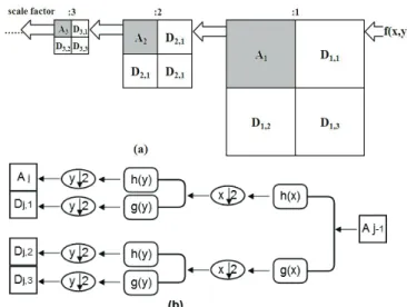
= + + + = = + + + + + + + + + + = = + + + + + + = = + + + = n j ,j ,j ,j n , , , , , , , , , , , , , , , , , , f D f D f D f A f D f D f D f D f D f D f D f D f D f A f D f D f D f D f D f D f A f D f D f D f A y x f 3 (8)

where Aj and Dj,p are the approximation coefficients and

detail coefficients obtained via wavelet decomposition, p=1, 2, 3, which respectively corresponds to detail coefficients of the horizontal, vertical and diagonal direction. Wavelet decomposition process is shown in Fig. 6a. The pyramid of level 0 is the original image. The jth_{-level pyramid is gotten from the (}_j_{− 1)}th_{- level pyramid}

by two steps as shown in Fig. 6b:

 Getting the (j − 1)th_{- level image by wavelet}

transform.

 Extracting the low-pass part of the resultant image from step  as the jth _{- level image.}

Figure 6 Wavelet decomposition and wavelet transform. (a) Wavelet decomposition of 2D image f(x, y). (b) The flowchart for wavelet

transform from (j− 1)th_{- level to}_jth_{- level.}

Here x↓_{2 and y}↓_{2 mean dyadic subsampling. If the}

(5)

that the signal frequency is high and more details of the image are given. If the scale factor is big, the signal frequency is low and the image is rough. As we know, significant areas usually correspond to high contrast areas, that is, the significant areas reflect the high frequency component in the frequency spectrum, and the background is corresponding to the low frequency components in the frequency spectrum. Therefore the background can be filtered via wavelet transform and the significance of salient region is improved.

Fig. 7 shows the experimental results of saliency map detected by wavelet pyramids, Gaussian pyramids and eye tracking equipment respectively. It can be seen that wavelet transform has a better effect on detecting saliency than Gaussian transform compared with the eye tracking results.

Figure 7 Performance comparisons: (a) Original images; (b) Saliency map detected by Wavelet Pyramids; (c) Saliency map detected by Gaussian Pyramids; (d) Saliency map detected by eye tracking equipment

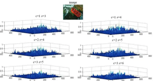
Figure 8 The similar data structure of a series of the feature maps (intensity) Further the pyramids based on wavelet decomposition

are used to extract feature maps by center-surround differences simulating center-surround receptive ﬁelds, which is obtained by calculating the difference between the center (c-level) pyramid and the surround (s-level) pyramid, shown from Eq. (9).

( )

( ) ( )

( )

, , , , , ) ( , ) , ) ( ( I c s I c I s RG c s RG c RG s BY c s BY c Y s O c s O c O s B θ θ θ Θ = Θ = Θ = = Θ (9)

Here, c and s indicate central level and surround level,

{

1,2,3 ,

}

,

{ }

2,3

c

∈

s c

= +

δ δ

∈

, which means there are six pairs of center-surround scales for each feature, and θ is the orientation of Gabor kernel function, as above. Θ is center-surround differences operator. This operation across spatial scales is done by interpolation to the fine scale and then point-by-point subtraction, yielding the feature map.

In summary, differences between "center" fine scales and its "surround" coarser scales create respectively 6 feature maps for intensity, red-green color-opponency, blue-yellow color-opponency, and the 8 orientations. A total of 66 feature maps are thus produced

The map combining the different center scales of feature maps by combination strategy is called "conspicuity map". In Itti’s model the linear combination strategy was used to calculate conspicuity maps, that is, the conspicuity map is simply the average of these feature maps.

After analyzing the data of a series of the feature maps corresponding to the same feature, it is obvious that the various feature maps have similar data structure, which is shown as Fig. 8. According to image multi-resolution analysis theory, scale changes from big to small, the corresponding frequency will change from low to high, contrast sensitivity function is proposed to combine the feature maps into a conspicuity map for each feature, which is elaborated by the following six steps:

 Normalize all feature maps to the range [0 1] to eliminate across-scale amplitude differences.

(6)

spectrogram.

 For each pixel P, calculate its visual spatial frequency f from Eq. (10):

. 2 2 y x f f f = + (10) Here, , , _α α 'v f ' u f_x = _y = (11) , 2 , 2 n v 'v m u ' u= − = − (12) where, fx is horizontal spatial frequency, fy is vertical spatial

frequency, α is angle of view, which depends on the experiment, m and n is the size of the image, (u, v) is the value of the point Q in the spectrum graph corresponding to the point P in the spatial domain.

 For each pixel P, calculate its contrast sensitivity function A(f) from Eq. (13) proposed by Manos and Sakrison, as shown in Fig. 9:

. )e 114 0 0192 0 ( 6 2 ) (_f _, _, _, _f (0,114 f)1,1 A ₌ _× ₊ _× − × ₍₁₃₎

Figure 9 Contrast sensitivity function

 Calculate the weight Wc of each contrast map by

averaging the value of all A(f), as shown in Eq. (14):

( )

_{( )}_, 1 1 1 n m i j j i c W A f m n = = = ×

∑∑

,

(14) where m and n are the size of the contrast map,

{

1,2,3

}

c

∈

.

 Combine contrast maps F into a conspicuity map C by Eq. (15):

( )

3 1 3 1 C i i i k i i N F W W = =  ×    =

∑

,

(15)

where N(.) is a normalization operator.

{

, , ,

}

k

∈

I BY RG O

θ , . 8 π 7 , 8 π 6 , 8 π 5 , 8 π 4 , 8 π 3 , 8 π 2 , 8 π 1 0       ∈ , θ

For example, the weights Wc of intensity feature maps

calculated via the above algorithm are shown in Tab. 1. Table 1 Weight Wi of each feature map (intensity feature)

Item No 1 No 2 No 3 No 4 No 5 No 6

c-s

level sc=3 =1 cs=4 =1 sc=4 =2 cs=5 =2 cs=3 =5 cs=3 =6 weight

Wc / % 21,6 20,6 18,2 15,3 12,9 11,4

2.3 Establishment of saliency map

Most of natural images have multiple visual features. Different features offer different significance. The more significant the feature is, the easier the significant areas are detected.

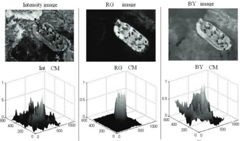
Figure 10 The data structures of the conspicuity maps: (a) intensity feature and conspicuity map; (b) red/green colour-opponency and conspicuity map; (c) blue/yellow colour-opponency and conspicuity map

(7)

Fig. 10 shows the data structures of intensity conspicuity map, RG conspicuity map and BY conspicuity map. It is obvious that different features have different conspicuity maps. The final saliency map is yielded by combining these conspicuity maps with different weights ω_i, which is clearly different from Itti's model. The weights are proportional to the contribution rate of each conspicuity map to the final saliency map. The details of weights calculation are as follows:

 Normalize each conspicuity map to the range [0 1], in order to eliminate amplitude differences due to dissimilar feature extraction mechanisms;

 For each conspicuity map, find its global maximum M and the average mof all the local maxima except for M;

 Globally multiply the conspicuity map from Eq. (16):

(

)

2. k k k = M −m ω (16) Here,

{

, , ,

}

k

∈

I BY RG O

θ . . 8 π 7 , 8 π 6 , 8 π 5 , 8 π 4 , 8 π 3 , 8 π 2 , 8 π 1 0       ∈ , θ

The total saliency S is given as Eq. (17), which is a combination of one intensity conspicuity map, two colour conspicuity maps and 8 orientation conspicuity maps.

(

)

S k k k k k C ω ω × =

∑

. (17) 3 Experimental results

In order to verify the credibility of our algorithm, a subjective experiment has been performed. We track and record the real eye movements of subjects by eye movement tracking experiment. 235 natural colour images with various contents selected from the Corel Photo Library and NeuroMathComp research group [18] are used as the test images. The size of the images is 640×480.

Figure 11 iView X Hi-speed eye movement tracking system iView X Hi-speed eye movement tracking system (analysis software: iView X v3.2) from Senso Motoric Instruments company (Germany) was used, and Dell 15

inch monitor was used to display the test images. 18 participants attended the experiment, all participants were normal vision, no colour blindness or colour weakness. The head of subject was fixed to ensure the eye track accuracy during the experiment. The eyes and screen centre were located at the same horizontal line, the observation distance was 2,5 times of the image height, about 0,65 meters. The image was displayed on the centre of the screen, the rest part of the screen was filled with black background. The tested images are shown in random order for the different testers, each image displayed for 5 seconds and between each image a grey image is displayed for 0,5 seconds. Experimental situation is shown in Fig. 11.

Figure 12 Performance comparison: (a) original images; (b) saliency maps by eye tracking; (c) saliency map by the proposed method;

(d) saliency maps obtained by Itti’s model.

Fig. 12 shows the experimental results of 5 tested images, each row in Fig. 12 indicates original image, eye tracking result, the results of our algorithm and the result of Itti’s model separately. Through comparing the eye tracking results with the concern degree by our method and Itti’s model, it can be seen that the saliency map obtained by our model is obviously much closer to the eye tracking results than Itti’s model. It shows that our proposed model produces a better visual effect than Itti’s model.

Table 2 Average computational complexity comparison

Image name Itti’s model (ms) our model (ms)

plane 98,8 47,6 tree 99,0 41,9 boat 100,9 42,1 bird 94,6 44,8 dragonfly 101,4 43,2 Average time 98,9 43,9

Furthermore, the improved model provides a significant improvement in computational complexity, as shown in Tab. 2.

The time for processing an image is performed by Matlab 2010 on DELL 620 (Microsoft Windows XP platform).

(8)

4 Conclusion

An improved visual attention model is proposed in this paper. In the improved model, one intensity, 2 color-opponency and 8 orientations of image are extracted in CIELa*b* colour space. The pyramids are given by wavelet decomposition which is more in accord with HVS. The various conspicuity maps are combined into a saliency map via combination strategy with different weights proportional to the contribution rate of each conspicuity map to the final saliency map. Experimental results show that the improved model has better performance and lower computational complexity than Itti's model. The proposed model is more promising to be employed to process multimedia in real time due to its low computational complexity and good accuracy.

Acknowledgment

This project is funded by the National Key Basic Research Program of China, No. 2010CB327705, and the National High Technology Research and Development

Program of China, No. 2012AA03A302，_{and innovation}

in higher education disciplines introduction program (B07027). And this project is also supported by Shenzhen China Star Optoelectronics Technology Co. LTD. The authors are grateful to the volunteers for participating in the experiments.

5 References

[1] Braun, J.; Sagi, D. Vision outside the focus of attention. // Percept Psychophysics. 48, 1(1990), pp. 45-48.

[2] Bruce, N. D.; Tsotsos, J. K. Saliency based on information maximization. // Adv. Neural Inf. Process. Syst. 18, (2006), pp. 155-162.

[3] Gao, D.; Vasconcelos, N. Bottom-up saliency is a discriminant process. // in Proc. IEEE Int. Conf. Computer Vision, 2007.

[4] Gopalakrishnan, V.; Hu, Y.; Rajan, D. Salient region detection by modeling distributions of colour and orientation. // IEEE Trans. Multi-media. 11, 5(2009), pp. 892-905.

[5] Guo, C.; Ma, Q.; Zhang, L. Spatio-temporal saliency detectionusing phase spectrum of quaternion Fourier transform. // in Proc. IEEE Int. Conf. Computer Vision and Pattern Recognition, 2008.

[6] Harel, J.; Koch, C.; Perona, P. Graph-based visual saliency. // Adv. Neural Inf. Process. Syst. 19, (2006), pp. 545-552. [7] He, D. J.; Zhang, Y. M.; Song, H. B. A Novel Saliency Map

Extraction Method Based on Improved Itti’s Model. // IEEE Computer Society. 3, (2010), pp. 323-327.

[8] Hou, X.; Zhang, L. Saliency detection: A spectral residual approach. // in Proc. IEEE Int. Conf. Computer Vision and Pattern Recognition, 2007.

[9] Hurvich, L. M.; Jameson, D. An opponent-process theory of colour vision. // Psychological Review. 64, 6(1957), pp. 384-404.

[10]Itti, L.; Koch, C.; Niebur, E. A model of saliency-based visual attention for rapid scene analysis. // IEEE Trans. Pattern Anal. Mach. Intell. 20, 11(1998), pp. 1254-1259. [11]Itti, L. Models of bottom-up and top-down visual attention.

// Ph.D. dissertation, Dept. Comput. Neural Syst., California Inst. Technol., Pasadena, 2000.

[12]Kanan, C.; Tong, M.; Zhang, L.; Cottrell, G. SUN:

Top-down saliency using natural statistics. // Visual Cognit. 17, 6(2009), pp. 979-1003.

[13]Lu, Z.; Lin, W.; Yang, X.; Ong, E.; Yao, S. Modeling visual attention’s modulatory aftereffects on visual sensitivity and quality evaluation. // IEEE Trans. Image Process. 14, 11(2005), pp. 1928-1942.

[14]Liu, T.; Sun, J.; Zheng, N.; Tang, X.; Shum, H. Y. Learning to detect a salient object. // in Proc. IEEE Int. Conf. Computer Vision and Pattern Recognition, 2007.

[15]Itti, L.; Koch, C. Computational modeling of visual attention. // Nature Rev. Neurosci. 2, 3(2001), pp. 194-203. [16]Torralba, A.; Oliva, A.; Castelhano, M. S.; Henderson, J. M. Contextual guidance of eye movements and attention in real-world scenes: The role of global features in object search. // Psychol. Rev. 113, 4(2006), pp. 766-786.

[17]Treisman, A.; Gelade, G. A feature-integration theory of attention. // Cognit. Psychol. 12, 1(1980), pp. 97-136. [18]http://www-sop.inria.fr/members/Neil.Bruce/#BIO

[19]Wolfe, J. M.; Butcher, S. J.; Hyle, M. Changing your mind: On the contributions of top-down and bottom-up guidance in visual search for feature singletons. // J. Experiment. Psychol.: Human Percept. Perform. 29, (2003), pp. 483-502. [20]Vuylsteke, P.; Schoeters, E. Multiscale image contrast

amplification (MUSICA™). // in Proc. SPIE Image Processing. 2167, (1994), pp. 551-560.

[21]Stahl, M.; Aach, T.; Buzug, T. M.; Dippel, S.; Neitzel, U. Noise-resistant weak-structure enhancement for digital radiography. // in Proc. SPIE Med. Imag. 3661, (1999), pp. 1406-1417.

[22]Lu, J.; Healy, D. M.; Weaver, J. B. Contrast enhancement of medical images using multiscale edge representation. // Opt. Eng. 33, 7(1994), pp. 2151-2161.

[23]Laine, A.; Fan, J.; Yang, W. Wavelets for contrast enhancement of digital mammography,. // IEEE Eng. Med. Biol. Mag. 14, (Sept./Oct. 1995), pp. 536-550.

[24]Zong, X.; Laine, A. F.; Geiser, E. A.; Wilson, D. C. De-noising and contrast enhancement via wavelet shrinkage and nonlinear adaptive gain. // in Proc. SPIE Wavelet Applications III. 2762, (1996), pp 566-574.

[25]Bolet, J.-P.; Cowen, A. R.; Launders, J.; Davies, A. G.; Parkin, G. J. S.; Bury, R. F. Progress with an "all-wavelet" approach to image enhancement and de-noising of direct digital thorax radiographic images. // in Proc. 6th_{Int. Conf.}

Image Processing and its Applications. 1, pp. 244-248, Dublin, Ireland, 1997, Conf. Publ. 443.