HAL Id: hal-01153255
https://hal.archives-ouvertes.fr/hal-01153255
Submitted on 19 May 2015
HAL
is a multi-disciplinary open access
archive for the deposit and dissemination of
sci-entific research documents, whether they are
pub-lished or not. The documents may come from
teaching and research institutions in France or
abroad, or from public or private research centers.
L’archive ouverte pluridisciplinaire
HAL
, est
destinée au dépôt et à la diffusion de documents
scientifiques de niveau recherche, publiés ou non,
émanant des établissements d’enseignement et de
recherche français ou étrangers, des laboratoires
publics ou privés.
Distributed under a Creative Commons
Attribution - NonCommercial - NoDerivatives| 4.0
A hybrid algorithm for Bayesian network structure
learning with application to multi-label learning
Maxime Gasse, Alex Aussem, Haytham Elghazel
To cite this version:
Maxime Gasse, Alex Aussem, Haytham Elghazel. A hybrid algorithm for Bayesian network structure
learning with application to multi-label learning. Expert Systems with Applications, Elsevier, 2014,
41 (15), pp.6755-6772. �10.1016/j.eswa.2014.04.032�. �hal-01153255�
A hybrid algorithm for Bayesian network structure learning
with application to multi-label learning
Maxime Gasse, Alex Aussem∗, Haytham Elghazel
Universit´e de Lyon, CNRS
Universit´e Lyon 1, LIRIS, UMR5205, F-69622, France
Abstract
We present a novel hybrid algorithm for Bayesian network structure learning, called H2PC. It first reconstructs the skeleton of a Bayesian network and then performs a Bayesian-scoring greedy hill-climbing search to orient the edges. The algorithm is based on divide-and-conquer constraint-based subroutines to learn the local structure around a target variable. We conduct two series of experimental comparisons of H2PC against Max-Min Hill-Climbing (MMHC), which is currently the most powerful state-of-the-art algorithm for Bayesian network structure learning. First, we use eight well-known Bayesian network benchmarks with various data sizes to assess the quality of the learned structure returned by the algorithms. Our extensive experiments show that H2PC outperforms MMHC in terms of goodness of fit to new data and quality of the network structure with respect to the true dependence structure of the data. Second, we investigate H2PC’s ability to solve the multi-label learning problem. We provide theoretical results to characterize and identify graphically the so-called minimal label powersets that appear as irreducible factors in the joint distribution under the faithfulness condition. The multi-label learning problem is then decomposed into a series of multi-class classification problems, where each multi-class variable encodes a label powerset. H2PC is shown to compare favorably to MMHC in terms of global classification accuracy over ten multi-label data sets covering
different application domains. Overall, our experiments support the conclusions that local structural learning with
H2PC in the form of local neighborhood induction is a theoretically well-motivated and empirically effective learning
framework that is well suited to multi-label learning. The source code (inR) of H2PC as well as all data sets used for
the empirical tests are publicly available.
Keywords: Bayesian networks, Multi-label learning, Markov boundary, Feature subset selection.
1. Introduction
A Bayesian network (BN) is a probabilistic model formed by a structure and parameters. The structure of a BN is a directed acyclic graph (DAG), whilst its parameters are conditional probability distributions as-sociated with the variables in the model. The problem of finding the DAG that encodes the conditional inde-pendencies present in the data attracted a great deal of interest over the last years (Rodrigues de Morais & Aussem, 2010a; Scutari, 2010; Scutari & Brogini, 2012; Kojima et al., 2010; Perrier et al., 2008; Villanueva & Maciel, 2012; Pe˜na, 2012; Gasse et al., 2012). The in-ferred DAG is very useful for many applications, includ-ing feature selection (Aliferis et al., 2010; Pe˜na et al.,
∗Corresponding author
Email address:[email protected](Alex Aussem)
2007; Rodrigues de Morais & Aussem, 2010b), causal relationships inference from observational data (Ellis & Wong, 2008; Aliferis et al., 2010; Aussem et al., 2012, 2010; Prestat et al., 2013; Cawley, 2008; Brown & Tsamardinos, 2008) and more recently multi-label learning (DembczyÅski et al., 2012; Zhang & Zhang, 2010; Guo & Gu, 2011).
Ideally the DAG should coincide with the dependence structure of the global distribution, or it should at least identify a distribution as close as possible to the correct one in the probability space. This step, called structure learning, is similar in approaches and terminology to model selection procedures for classical statistical mod-els. Basically, constraint-based (CB) learning methods systematically check the data for conditional indepen-dence relationships and use them as constraints to con-struct a partially oriented graph representative of a BN
equivalence class, whilst search-and-score (SS) meth-ods make use of a goodness-of-fit score function for evaluating graphical structures with regard to the data set. Hybrid methods attempt to get the best of both worlds: they learn a skeleton with a CB approach and constrain on the DAGs considered during the SS phase. In this study, we present a novel hybrid algorithm for
Bayesian network structure learning, called H2PC1. It
first reconstructs the skeleton of a Bayesian network and then performs a Bayesian-scoring greedy hill-climbing search to orient the edges. The algorithm is based on divide-and-conquer constraint-based subroutines to learn the local structure around a target variable. HPC may be thought of as a way to compensate for the large number of false negatives at the output of the weak PC learner, by performing extra computations. As this may arise at the expense of the number of false positives, we control the expected proportion of false discover-ies (i.e. false positive nodes) among all the discoverdiscover-ies
made inPCT. We use a modification of the Incremental
association Markov boundary algorithm (IAMB), ini-tially developed by Tsamardinos et al. in (Tsamardi-nos et al., 2003) and later modified by Jose Pe˜na in (Pe˜na, 2008) to control the FDR of edges when learn-ing Bayesian network models. HPC scales to thou-sands of variables and can deal with many fewer
sam-ples (n < q). To illustrate its performance by means
of empirical evidence, we conduct two series of exper-imental comparisons of H2PC against Max-Min Hill-Climbing (MMHC), which is currently the most pow-erful state-of-the-art algorithm for BN structure learn-ing (Tsamardinos et al., 2006), uslearn-ing well-known BN benchmarks with various data sizes, to assess the good-ness of fit to new data as well as the quality of the network structure with respect to the true dependence structure of the data.
We then address a real application of H2PC where the true dependence structure is unknown. More specif-ically, we investigate H2PC’s ability to encode the joint distribution of the label set conditioned on the input features in the multi-label classification (MLC) prob-lem. Many challenging applications, such as photo and video annotation and web page categorization, can ben-efit from being formulated as MLC tasks with large number of categories (DembczyÅski et al., 2012; Read et al., 2009; Madjarov et al., 2012; Kocev et al., 2007; Tsoumakas et al., 2010b). Recent research in MLC fo-cuses on the exploitation of the label conditional
de-1A first version of HP2C without FDR control has been discussed
in a paper that appeared in the Proceedings of ECML-PKDD, pages 58-73, 2012.
pendency in order to better predict the label combina-tion for each example. We show that local BN
struc-ture discovery methods offer an elegant and
power-ful approach to solve this problem. We establish two theorems (Theorem 6 and 7) linking the concepts of marginal Markov boundaries, joint Markov boundaries and so-called label powersets under the faithfulness
as-sumption. These Theorems offer a simple guideline to
characterize graphically : i) the minimal label powerset
decomposition, (i.e. into minimal subsetsYLP⊆Ysuch
thatYLP ⊥⊥Y\YLP |X), and ii) the minimal subset of
features, w.r.t an Information Theory criterion, needed to predict each label powerset, thereby reducing the in-put space and the comin-putational burden of the multi-label classification. To solve the MLC problem with BNs, the DAG obtained from the data plays a pivotal role. So in this second series of experiments, we assess the comparative ability of H2PC and MMHC to encode the label dependency structure by means of an indirect
goodness of fit indicator, namely the 0/1 loss function,
which makes sense in the MLC context.
The rest of the paper is organized as follows: In the Section 2, we review the theory of BN and dis-cuss the main BN structure learning strategies. We then present the H2PC algorithm in details in Section 3. Sec-tion 4 evaluates our proposed method and shows results for several tasks involving artificial data sampled from known BNs. Then we report, in Section 5, on our exper-iments on real-world data sets in a multi-label learning context so as to provide empirical support for the pro-posed methodology. The main theoretical results appear formally as two theorems (Theorem 8 and 9) in Section 5. Their proofs are established in the Appendix. Fi-nally, Section 6 raises several issues for future work and we conclude in Section 7 with a summary of our contri-bution.
2. Preliminaries
We define next some key concepts used along the pa-per and state some results that will support our analysis. In this paper, upper-case letters in italics denote random
variables (e.g.,X,Y) and lower-case letters in italics
de-note their values (e.g.,x,y). Upper-case bold letters
de-note random variable sets (e.g.,X,Y,Z) and lower-case
bold letters denote their values (e.g.,x,y). We denote
byX⊥⊥Y|Zthe conditional independence betweenX
andYgiven the set of variablesZ. To keep the notation
2.1. Bayesian networks
Formally, a BN is a tuple< G,P >, whereG =<
U,E >is a directed acyclic graph (DAG) with nodes
representing the random variablesUandPa joint
prob-ability distribution in U. In addition, Gand P must
satisfy the Markov condition: every variable, X ∈ U,
is independent of any subset of its non-descendant vari-ables conditioned on the set of its parents, denoted by
PaGi. From the Markov condition, it is easy to prove
(Neapolitan, 2004) that the joint probability distribution
Pon the variables inUcan be factored as follows :
P(V)=P(X1, . . . ,Xn)= n Y i=1 P(Xi|Pa G i) (1)
Equation 1 allows a parsimonious decomposition of
the joint distributionP. It enables us to reduce the
prob-lem of determining a huge number of probability values to that of determining relatively few.
A BN structureGentails a set of conditional
indepen-dence assumptions. They can all be identified by the
d-separation criterion(Pearl, 1988). We useX⊥GY|Zto
denote the assertion thatXis d-separated fromY given
ZinG. Formally,X⊥GY|Zis true when for every
undi-rected path inGbetweenX andY, there exists a node
W in the path such that either (1)W does not have two
parents in the path andW ∈Z, or (2)Whas two parents
in the path and neitherWnor its descendants is inZ. If
<G,P>is a BN,X⊥PY|ZifX⊥G Y|Z. The converse
does not necessarily hold. We say that<G,P >
satis-fies thefaithfulness conditionif the d-separations inG
identifyall and onlythe conditional independencies in
P, i.e.,X⊥PY|ZiffX⊥GY|Z.
A Markov blanketMT ofT is any set of variables
such thatT is conditionally independent of all the
re-maining variables givenMT. By extension, a Markov
blanket ofT inVguarantees thatMT ⊆V, and thatT
is conditionally independent of the remaining variables
inV, givenMT. A Markov boundary,MBT, ofT is any
Markov blanket such that none of its proper subsets is a
Markov blanket ofT.
We denote byPCGT, the set of parents and children
ofT inG, and by SPGT, the set ofspousesofT inG.
ThespousesofT are the variables that have common
children withT. These sets are unique for allG, such
that<G,P>satisfies the faithfulness condition and so
we will drop the superscriptG. We denote bydSep(X),
the set that d-separatesXfrom the (implicit) targetT.
Theorem 1. Suppose<G,P>satisfies the faithfulness
condition. Then X and Y are not adjacent inGiff∃Z∈
U\ {X,Y}such that X ⊥⊥ Y | Z. Moreover, MBX =
PCX∪SPX.
A proof can be found for instance in (Neapolitan, 2004).
Two graphs are said equivalentiff they encode the
same set of conditional independencies via the d-separation criterion. The equivalence class of a DAG
Gis a set of DAGs that are equivalent toG. The next
result showed by (Pearl, 1988), establishes that equiv-alent graphs have the same undirected graph but might disagree on the direction of some of the arcs.
Theorem 2. Two DAGs are equivalent iffthey have the
same underlying undirected graph and the same set of v-structures (i.e. converging edges into the same node,
such as X →Y ←Z).
Moreover, an equivalence class of network structures can be uniquely represented by a partially directed DAG (PDAG), also called a DAG pattern. The DAG pattern is defined as the graph that has the same links as the DAGs in the equivalence class and has oriented all and only the edges common to the DAGs in the equivalence class. A structure learning algorithm from data is said to be correct (or sound) if it returns the correct DAG pattern (or a DAG in the correct equivalence class) under the assumptions that the independence tests are reliable and that the learning database is a sample from a distribution
Pfaithful to a DAGG, The (ideal) assumption that the
independence tests are reliable means that they decide
(in)dependence iffthe (in)dependence holds inP.
2.2. Conditional independence properties
The following three theorems, borrowed from Pe˜na et al. (2007), are proven in Pearl (1988):
Theorem 3. Let X,Y,Z and W denote four
mutu-ally disjoint subsets of U. Any probability
distribu-tion p satisfies the following four properties:
Symme-try X ⊥⊥ Y | Z ⇒ Y ⊥⊥ X | Z, Decomposition,
X ⊥⊥ (Y∪W) | Z ⇒ X ⊥⊥ Y | Z, Weak Union
X⊥⊥(Y∪W)|Z⇒X⊥⊥Y|(Z∪W)and Contraction,
X⊥⊥Y|(Z∪W)∧X⊥⊥W|Z⇒X⊥⊥(Y∪W)|Z.
Theorem 4. If p is strictly positive, then p satisfies the
previous four properties plus the Intersection property
X ⊥⊥Y| (Z∪W)∧X ⊥⊥ W| (Z∪Y) ⇒ X ⊥⊥ (Y∪
W)|Z. Additionally, eachX∈Uhas a unique Markov
boundary,MBX
Theorem 5. If p is faithful to a DAGG, then p satisfies
the previous five properties plus the Composition
prop-ertyX⊥⊥Y|Z∧X⊥⊥W|Z⇒X⊥⊥(Y∪W)|Zand
the local Markov property X ⊥⊥(NDX\PaX)|PaX for
each X ∈ U, whereNDX denotes the non-descendants
2.3. Structure learning strategies
The number of DAGs,G, is super-exponential in the
number of random variables in the domain and the
prob-lem of learning the most probablea posterioriBN from
data is worst-case NP-hard (Chickering et al., 2004). One needs to resort to heuristical methods in order to
be able to solve very large problems effectively.
Both CB and SS heuristic approaches have advan-tages and disadvanadvan-tages. CB approaches are relatively quick, deterministic, and have a well defined stopping criterion; however, they rely on an arbitrary significance level to test for independence, and they can be unsta-ble in the sense that an error early on in the search
can have a cascading effect that causes many errors to
be present in the final graph. SS approaches have the advantage of being able to flexibly incorporate users’ background knowledge in the form of prior probabili-ties over the structures and are also capable of dealing with incomplete records in the database (e.g. EM tech-nique). Although SS methods are favored in practice when dealing with small dimensional data sets, they are slow to converge and the computational complexity of-ten prevents us from finding optimal BN structures (Per-rier et al., 2008; Kojima et al., 2010). With currently available exact algorithms (Koivisto & Sood, 2004; Si-lander & Myllym¨aki, 2006; Cussens & Bartlett, 2013; Studen´y & Haws, 2014) and a decomposable score like BDeu, the computational complexity remains exponen-tial, and therefore, such algorithms are intractable for BNs with more than around 30 vertices on current work-stations. For larger sets of variables the computational burden becomes prohibitive and restrictions about the structure have to be imposed, such as a limit on the size of the parent sets. With this in mind, the ability to restrict the search locally around the target variable is a key advantage of CB methods over SS methods. They are able to construct a local graph around the tar-get node without having to construct the whole BN first, hence their scalability (Pe˜na et al., 2007; Rodrigues de Morais & Aussem, 2010b,a; Tsamardinos et al., 2006; Pe˜na, 2008).
With a view to balancing the computation cost with the desired accuracy of the estimates, several hybrid methods have been proposed recently. Tsamardinos et al. proposed in (Tsamardinos et al., 2006) the Min-Max Hill Climbing (MMHC) algorithm and conducted one of the most extensive empirical comparison per-formed in recent years showing that MMHC was the fastest and the most accurate method in terms of struc-tural error based on the strucstruc-tural hamming distance. More specifically, MMHC outperformed both in terms
of time efficiency and quality of reconstruction the PC
(Spirtes et al., 2000), the Sparse Candidate (Friedman et al., 1999b), the Three Phase Dependency Analysis (Cheng et al., 2002), the Optimal Reinsertion (Moore & Wong, 2003), the Greedy Equivalence Search (Chick-ering, 2002), and the Greedy Hill-Climbing Search on a variety of networks, sample sizes, and parameter val-ues. Although MMHC is rather heuristic by nature (it returns a local optimum of the score function), it is cur-rently considered as the most powerful state-of-the-art algorithm for BN structure learning capable of dealing with thousands of nodes in reasonable time.
In order to enhance its performance on small dimen-sional data sets, Perrier et al. proposed in (Perrier et al.,
2008) a hybrid algorithm that can learn anoptimalBN
(i.e., it converges to the true model in the sample limit) when an undirected graph is given as a structural con-straint. They defined this undirected graph as a super-structure (i.e., every DAG considered in the SS phase is compelled to be a subgraph of the super-structure). This algorithm can learn optimal BNs containing up to 50 vertices when the average degree of the super-structure is around two, that is, a sparse structural constraint is assumed. To extend its feasibility to BN with a few hundred of vertices and an average degree up to four, Kojima et al. proposed in (Kojima et al., 2010) to divide the super-structure into several clusters and perform an optimal search on each of them in order to scale up to larger networks. Despite interesting improvements in terms of score and structural hamming distance on sev-eral benchmark BNs, they report running times about
103times longer than MMHC on average, which is still
prohibitive.
Therefore, there is great deal of interest in hybrid methods capable of improving the structural accuracy of both CB and SS methods on graphs containing up to thousands of vertices. However, they make the strong assumption that the skeleton (also called super-structure) contains at least the edges of the true network and as small as possible extra edges. While control-ling the false discovery rate (i.e., false extra edges) in BN learning has attracted some attention recently (Ar-men & Tsamardinos, 2011; Pe˜na, 2008; Tsamardinos & Brown, 2008), to our knowledge, there is no work on controlling actively the rate of false-negative errors (i.e., false missing edges).
2.4. Constraint-based structure learning
Before introducing the H2PC algorithm, we discuss the general idea behind CB methods. The induction of local or global BN structures is handled by CB methods through the identification of local neighborhoods (i.e.,
data sets. CB methods systematically check the data for conditional independence relationships in order to in-fer a target’s neighborhood. Typically, the algorithms
run either aG2or aχ2independence test when the data
set is discrete and a Fisher’s Z test when it is continu-ous in order to decide on dependence or independence, that is, upon the rejection or acceptance of the null hy-pothesis of conditional independence. Since we are limiting ourselves to discrete data, both the global and the local distributions are assumed to be multinomial, and the latter are represented as conditional probabil-ity tables. Conditional independence tests and network scores for discrete data are functions of these condi-tional probability tables through the observed frequen-cies{ni jk;i = 1, . . . ,R;j = 1, . . . ,C;k = 1, . . . ,L}for
the random variablesXandYand all the configurations
of the levels of the conditioning variablesZ. We use
ni+kas shorthand for the marginalPjni jk and similarly
forni+k,n++kandn+++=n. We use a classic conditional
independence test based on the mutual information. The mutual information is an information-theoretic distance measure defined as MI(X,Y|Z)= R X i=1 C X j=1 L X k=1 ni jk n log ni jkn++k ni+kn+jk
It is proportional to the log-likelihood ratio testG2
(they differ by a 2n factor, where n is the sample size).
The asymptotic null distribution isχ2with (R−1)(C−
1)Ldegrees of freedom. For a detailed analysis of their
properties we refer the reader to (Agresti, 2002). The main limitation of this test is the rate of convergence to its limiting distribution, which is particularly prob-lematic when dealing with small samples and sparse contingency tables. The decision of accepting or re-jecting the null hypothesis depends implicitly upon the degree of freedom which increases exponentially with the number of variables in the conditional set. Sev-eral heuristic solutions have emerged in the literature (Spirtes et al., 2000; Rodrigues de Morais & Aussem, 2010a; Tsamardinos et al., 2006; Tsamardinos & Bor-boudakis, 2010) to overcome some shortcomings of the asymptotic tests. In this study we use the two follow-ing heuristics that are used in MMHC. First, we do not
performMI(X,Y|Z) and assume independence if there
are not enough samples to achieve large enough power. We require that the average sample per count is above a user defined parameter, equal to 5, as in (Tsamardi-nos et al., 2006). This heuristic is called the power rule.
Second, we consider as structural zero either casen+jk
orni+k = 0. For example, ifn+jk = 0, we consider y
as a structurally forbidden value for Y when Z=z and
we reduce R by 1 (as if we had one column less in the
contingency table where Z=z). This is known as the
degrees of freedom adjustment heuristic. 3. The H2PC algorithm
In this section, we present our hybrid algorithm for Bayesian network structure learning, called Hy-brid HPC (H2PC). It first reconstructs the skeleton of a Bayesian network and then performs a Bayesian-scoring greedy hill-climbing search to filter and orient the edges. It is based on a CB subroutine called HPC to learn the parents and children of a single variable. So, we shall discuss HPC first and then move to H2PC. 3.1. Parents and Children Discovery
HPC (Algorithm 1) can be viewed as an ensemble method for combining many weak PC learners in an at-tempt to produce a stronger PC learner. HPC is based
on three subroutines: Data-Efficient Parents and
Chil-dren Superset(DE-PCS),Data-Efficient Spouses
Super-set(DE-SPS), andIncremental Association Parents and
Childrenwith false discovery rate control (FDR-IAPC),
a weak PC learner based on FDR-IAMB (Pe˜na, 2008) that requires little computation. HPC receives a target
nodeT, a data setDand a set of variablesUas input
and returns an estimation ofPCT. It is hybrid in that
it combines the benefits of incremental and divide-and-conquer methods. The procedure starts by extracting
a supersetPCST ofPCT (line 1) and a supersetSPST
of SPT (line 2) with a severe restriction on the
max-imum conditioning size (Z <= 2) in order to
signifi-cantly increase the reliability of the tests. A first can-didate PC set is then obtained by running the weak PC
learner called FDR-IAPC onPCST∪SPST(line 3). The
key idea is the decentralized search at lines 4-8 that in-cludes, in the candidate PC set, all variables in the
su-perset PCST \PCT that haveT in their vicinity. So,
HPC may be thought of as a way to compensate for the large number of false negatives at the output of the weak PC learner, by performing extra computations. Note
that, in theory, X is in the output of FDR-IAPC(Y) if
and only ifY is in the output of FDR-IAPC(X).
How-ever, in practice, this may not always be true, particu-larly when working in high-dimensional domains (Pe˜na, 2008). By loosening the criteria by which two nodes are
said adjacent, the effective restrictions on the size of the
neighborhood are now far less severe. The decentral-ized search has a significant impact on the accuracy of HPC as we shall see in in the experiments. We proved in
(Rodrigues de Morais & Aussem, 2010a) that the orig-inal HPC(T) is consistent, i.e. its output converges in
probability toPCT , if the hypothesis tests are
consis-tent. The proof also applies to the modified version pre-sented here.
We now discuss the subroutines in more detail. FDR-IAPC (Algorithm 2) is a fast incremental method that
receives a data set Dand a target nodeT as its input
and promptly returns a rough estimation ofPCT, hence
the term “weak” PC learner. In this study, we use FDR-IAPC because it aims at controlling the expected pro-portion of false discoveries (i.e., false positive nodes in
PCT) among all the discoveries made. FDR-IAPC is a
straightforward extension of the algorithm IAMBFDR developed by Jose Pe˜na in (Pe˜na, 2008), which is itself a modification of the incremental association Markov boundary algorithm (IAMB) (Tsamardinos et al., 2003), to control the expected proportion of false discover-ies (i.e., false positive nodes) in the estimated Markov boundary. FDR-IAPC simply removes, at lines 3-6, the
spousesSPTfrom the estimated Markov boundaryMBT
output by IAMBFDR at line 1, and returnsPCT
assum-ing the faithfulness condition.
The subroutines DE-PCS (Algorithm 3) and DE-SPS
(Algorithm 4) search a superset ofPCTandSPT
respec-tively with a severe restriction on the maximum
condi-tioning size (|Z|<=1 in DE-PCS and|Z|<=2 in
DE-SPS) in order to significantly increase the reliability of the tests. The variable filtering has two advantages : i) it allows HPC to scale to hundreds of thousands of variables by restricting the search to a subset of relevant variables, and ii) it eliminates many true or approximate deterministic relationships that produce many false neg-ative errors in the output of the algorithm, as explained in (Rodrigues de Morais & Aussem, 2010b,a). DE-SPS works in two steps. First, a growing phase (lines 4-8) adds the variables that are d-separated from the target but still remain associated with the target when
condi-tioned on another variable fromPCST. The shrinking
phase (lines 9-16) discards irrelevant variables that are ancestors or descendants of a target’s spouse. Pruning such irrelevant variables speeds up HPC.
3.2. Hybrid HPC (H2PC)
In this section, we discuss the SS phase. The follow-ing discussion draws strongly on (Tsamardinos et al., 2006) as the SS phase in Hybrid HPC and MMHC are exactly the same. The idea of constraining the
search to improve time-efficiency first appeared in the
Sparse Candidate algorithm (Friedman et al., 1999b).
It results in efficiency improvements over the
(uncon-strained) greedy search. All recent hybrid algorithms
Algorithm 1HPC
Require: T: target;D: data set;U: set of variables Ensure: PCT: Parents and Children ofT
1: [PCST,dSep]←DE-PCS(T,D,U) 2: SPST ←DE-SPS(T,D,U,PCST,dSep) 3: PCT ←FDR-IAPC(T,D,(T∪PCST∪SPST)) 4: for allX∈PCST\PCTdo 5: ifT∈FDR-IAPC(X,D,(T∪PCST∪SPST))then 6: PCT ←PCT∪X 7: end if 8: end for Algorithm 2FDR-IAPC
Require: T: target;D: data set;U: set of variables Ensure: PCT: Parents and children ofT;
*Learn the Markov boundary of T
1: MBT←IAMBFDR(X,D,U) *Remove spouses of T fromMBT
2: PCT ←MBT
3: for allX∈MBTdo
4: if∃Z⊆(MBT\X) such thatT ⊥X|Z then
5: PCT ←PCT\X
6: end if 7: end for
Algorithm 3DE-PCS
Require: T: target;D: data set;U: set of variables; Ensure: PCST: parents and children superset ofT;dSep:
d-separating sets; Phase I:Remove X if T⊥X 1: PCST←U\T 2: for allX∈PCSTdo 3: if(T ⊥X)then 4: PCST←PCST\X 5: dSep(X)← ∅ 6: end if 7: end for
Phase II:Remove X if T⊥X|Y
8: for allX∈PCSTdo
9: for allY∈PCST\Xdo
10: if(T ⊥X|Y)then
11: PCST ←PCST\X
12: dSep(X)←Y
13: break loop FOR 14: end if
15: end for 16: end for
Algorithm 4DE-SPS
Require: T: target; D: data set; U: the set of variables;
PCST: parents and children superset of T; dSep:
d-separating sets;
Ensure: SPST: Superset of the spouses ofT;
1: SPST← ∅ 2: for allX∈PCSTdo 3: SPSX T← ∅ 4: for allY ∈U\ {T∪PCST}do 5: if(T 6⊥Y|dSep(Y)∪X)then 6: SPSXT←SPS X T∪Y 7: end if 8: end for 9: for allY ∈SPSX Tdo 10: for allZ∈SPSX T\Ydo 11: if(T ⊥Y|X∪Z)then 12: SPSX T ←SPS X T\Y
13: break loop FOR 14: end if 15: end for 16: end for 17: SPST←SPST∪SPSXT 18: end for Algorithm 5Hybrid HPC
Require: D: data set;U: set of variables Ensure: A DAGGon the variablesU
1: for allpair of nodesX,Y∈U do
2: Add X inPCYand Add Y inPCX ifX∈HPC(Y) and
Y∈HPC(X)
3: end for
4: Starting from an empty graph, perform greedy
hill-climbing with operatorsadd-edge, delete-edge,
reverse-edge. Only try operatoradd-edge X→YifY∈PCX
build on this idea, but employ a sound algorithm for identifying the candidate parent sets. The Hybrid HPC first identifies the parents and children set of each vari-able, then performs a greedy hill-climbing search in the space of BN. The search begins with an empty graph. The edge addition, deletion, or direction reversal that leads to the largest increase in score (the BDeu score with uniform prior was used) is taken and the search continues in a similar fashion recursively. The
impor-tant difference from standard greedy search is that the
search is constrained to only consider adding an edge if it was discovered by HPC in the first phase. We extend the greedy search with a TABU list (Friedman et al., 1999b). The list keeps the last 100 structures explored. Instead of applying the best local change, the best lo-cal change that results in a structure not on the list is performed in an attempt to escape local maxima. When 15 changes occur without an increase in the maximum score ever encountered during search, the algorithm ter-minates. The overall best scoring structure is then re-turned. Clearly, the more false positives the heuristic al-lows to enter candidate PC set, the more computational burden is imposed in the SS phase.
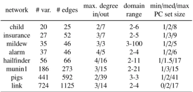
4. Experimental validation on synthetic data Before we proceed to the experiments on real-world multi-label data with H2PC, we first conduct an exper-imental comparison of H2PC against MMHC on syn-thetic data sets sampled from eight well-known bench-marks with various data sizes in order to gauge the prac-tical relevance of the H2PC. These BNs that have been previously used as benchmarks for BN learning algo-rithms (see Table 1 for details). Results are reported in terms of various performance indicators to investigate how well the network generalizes to new data and how well the learned dependence structure matches the true structure of the benchmark network. We implemented
H2PC inR(R Core Team, 2013) and integrated the code
into thebnlearnpackage from (Scutari, 2010). MMHC
was implemented by Marco Scutari in bnlearn. The
source code of H2PC as well as all data sets used for
the empirical tests are publicly available2. The
thresh-old considered for the type I error of the test is 0.05.
Our experiments were carried out on PC with Intel(R) Core(TM) i5-3470M CPU @3.20 GHz 4Go RAM run-ning under Linux 64 bits.
We do not claim that those data sets resemble real-world problems, however, they make it possible to
Table 1: Description of the BN benchmarks used in the experiments.
network # var. # edges max. degree domain min/med/max
in/out range PC set size
child 20 25 2/7 2-6 1/2/8 insurance 27 52 3/7 2-5 1/3/9 mildew 35 46 3/3 3-100 1/2/5 alarm 37 46 4/5 2-4 1/2/6 hailfinder 56 66 4/16 2-11 1/1.5/17 munin1 186 273 3/15 2-21 1/3/15 pigs 441 592 2/39 3-3 1/2/41 link 724 1125 3/14 2-4 0/2/17
pare the outputs of the algorithms with the known struc-ture. All BN benchmarks (structure and probability
ta-bles) were downloaded from the bnlearnrepository3.
Ten sample sizes have been considered: 50, 100, 200, 500, 1000, 2000, 5000, 10000, 20000 and 50000. All experiments are repeated 10 times for each sample size and each BN. We investigate the behavior of both algo-rithms using the same parametric tests as a reference. 4.1. Performance indicators
We first investigate the quality of the skeleton re-turned by H2PC during the CB phase. To this end, we measure the false positive edge ratio, the precision (i.e., the number of true positive edges in the output divided by the number of edges in the output), the recall (i.e., the number of true positive edges divided the true number of edges) and a combination of precision and recall
de-fined as p
(1−precision)2+(1−recall)2, to measure
the Euclidean distance from perfect precision and re-call, as proposed in (Pe˜na et al., 2007). Second, to as-sess the quality of the final DAG output at the end of the SS phase, we report the five performance indicators (Scutari & Brogini, 2012) described below:
• the posterior density of the network for the data
it was learned from, as a measure of goodness of fit. It is known as the Bayesian Dirichlet equivalent score (BDeu) from (Heckerman et al., 1995; Bun-tine, 1991) and has a single parameter, the equiv-alent sample size, which can be thought of as the size of an imaginary sample supporting the prior distribution. The equivalent sample size was set to 10 as suggested in (Koller & Friedman, 2009);
• the BIC score (Schwarz, 1978) of the network for
the data it was learned from, again as a measure of goodness of fit;
3http://www.bnlearn.com/bnrepository
• the posterior density of the network for a new data
set, as a measure of how well the network general-izes to new data;
• the BIC score of the network for a new data set,
again as a measure of how well the network gener-alizes to new data;
• the Structural Hamming Distance (SHD) between
the learned and the true structure of the network, as a measure of the quality of the learned depen-dence structure. The SHD between two PDAGs is defined as the number of the following operators required to make the PDAGs match: add or delete an undirected edge, and add, remove, or reverse the orientation of an edge.
For each data set sampled from the true probability distribution of the benchmark, we first learn a network structure with the H2PC and MMHC and then we com-pute the relevant performance indicators for each pair of network structures. The data set used to assess how well the network generalizes to new data is generated again from the true probability structure of the bench-mark networks and contains 50000 observations.
Notice that using the BDeu score as a metric of recon-struction quality has the following two problems. First, the score corresponds to the a posteriori probability of a network only under certain conditions (e.g., a Dirichlet distribution of the hyper parameters); it is unknown to what degree these assumptions hold in distributions en-countered in practice. Second, the score is highly sensi-tive to the equivalent sample size (set to 10 in our exper-iments) and depends on the network priors used. Since, typically, the same arbitrary value of this parameter is used both during learning and for scoring the learned network, the metric favors algorithms that use the BDeu score for learning. In fact, the BDeu score does not rely on the structure of the original, gold standard network at all; instead it employs several assumptions to score the networks. For those reasons, in addition to the score we also report the BIC score and the SHD metric.
4.2. Results
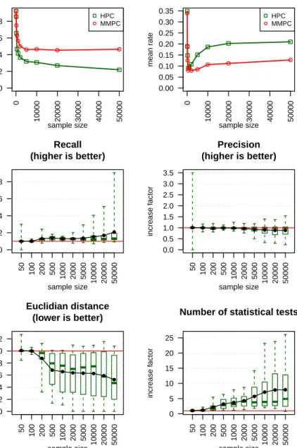
In Figure 1, we report the quality of the skeleton ob-tained with HPC over that obob-tained with MMPC (be-fore the SS phase) as a function of the sample size. Results for each benchmark are not shown here in de-tail due to space restrictions. For sake of conciseness, the performance values are averaged over the 8 bench-marks depicted in Table 1. The increase factor for a given performance indicator is expressed as the ratio of
0 10000 20000 30000 40000 50000 0.0 0.2 0.4 0.6 0.8 sample size mean r ate
False negative rate (lower is better) HPC MMPC 0 10000 20000 30000 40000 50000 0.00 0.05 0.10 0.15 0.20 0.25 0.30 0.35 sample size mean r ate
False positive rate (lower is better) HPC MMPC 50 100 200 500 1000 2000 5000 10000 20000 50000 0 2 4 6 8 sample size increase f actor Recall (higher is better) 50 100 200 500 1000 2000 5000 10000 20000 50000 0.0 0.5 1.0 1.5 2.0 2.5 3.0 3.5 sample size increase f actor Precision (higher is better) 50 100 200 500 1000 2000 5000 10000 20000 50000 0.0 0.2 0.4 0.6 0.8 1.0 1.2 sample size increase f actor Euclidian distance (lower is better) 50 100 200 500 1000 2000 5000 10000 20000 50000 0 5 10 15 20 25 sample size increase f actor
Number of statistical tests
Figure 1: Quality of the skeleton obtained with HPC over that obtained with MMPC (after the CB phase). The 2 first figures present mean values
aggregated over the 8 benchmarks. The 4 last figures present increase factors of HPC/MMPC, with the median, quartile, and most extreme values
the performance value obtained with HPC over that ob-tained with MMPC (the gold standard). Note that for some indicators, an increase is actually not an improve-ment but is worse (e.g., false positive rate, Euclidean distance). For clarity, we mention explicitly on the
sub-plots whether an increase factor> 1 should be
inter-preted as an improvement or not. Regarding the qual-ity of the superstructure, the advantages of HPC against MMPC are noticeable. As observed, HPC consistently increases the recall and reduces the rate of false neg-ative edges. As expected this benefit comes at a lit-tle expense in terms of false positive edges. HPC also improves the Euclidean distance from perfect precision and recall on all benchmarks, while increasing the num-ber of independence tests and thus the running time in the CB phase (see number of statistical tests). It is worth noting that HPC is capable of reducing by 50% the Eu-clidean distance with 50000 samples (lower left plot). These results are very much in line with other exper-iments presented in (Rodrigues de Morais & Aussem, 2010a; Villanueva & Maciel, 2012).
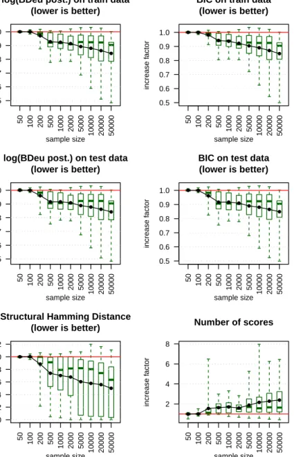
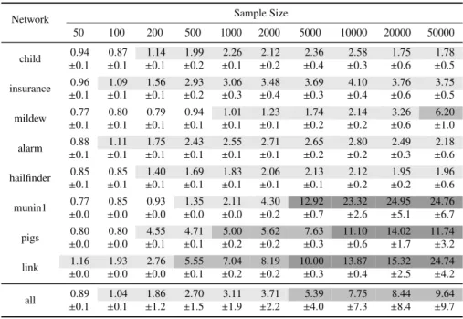
In Figure 2, we report the quality of the final DAG ob-tained with H2PC over that obob-tained with MMHC (af-ter the SS phase) as a function of the sample size. Re-garding BDeu and BIC on both training and test data, the improvements are noteworthy. The results in terms of goodness of fit to training data and new data using H2PC clearly dominate those obtained using MMHC, whatever the sample size considered, hence its ability to generalize better. Regarding the quality of the network structure itself (i.e., how close is the DAG to the true dependence structure of the data), this is pretty much a dead heat between the 2 algorithms on small sam-ple sizes (i.e., 50 and 100), however we found H2PC to perform significantly better on larger sample sizes. The SHD increase factor decays rapidly (lower is bet-ter) as the sample size increases (lower left plot). For 50 000 samples, the SHD is on average only 50% that of MMHC. Regarding the computational burden involved, we may observe from Table 2 that H2PC has a little computational overhead compared to MMHC. The run-ning time increase factor grows somewhat linearly with the sample size. With 50000 samples, H2PC is approxi-mately 10 times slower on average than MMHC. This is mainly due to the computational expense incurred in ob-taining larger PC sets with HPC, compared to MMPC. 5. Application to multi-label learning
In this section, we address the problem of multi-label learning with H2PC. MLC is a challenging prob-lem in many real-world application domains, where
each instance can be assigned simultaneously to mul-tiple binary labels (DembczyÅski et al., 2012; Read et al., 2009; Madjarov et al., 2012; Kocev et al., 2007; Tsoumakas et al., 2010b). Formally, learning from multi-label examples amounts to finding a mapping from a space of features to a space of labels. We shall
assume throughout thatX(a random vector inRd) is the
feature set, Y(a random vector in {0,1}n) is the label
set,U=X∪Yandpa probability distribution defined
overU. Given a multi-label training setD, the goal of
multi-label learning is to find a function which is able to map any unseen example to its proper set of labels. From the Bayesian point of view, this problem amounts
to modeling the conditional joint distributionp(Y|X).
5.1. Related work
This MLC problem may be tackled in various ways (Luaces et al., 2012; Alvares-Cherman et al., 2011; Read et al., 2009; Blockeel et al., 1998; Kocev et al., 2007). Each of these approaches is supposed to capture - to some extent - the relationships between labels. The two most straightforward meta-learning methods (Mad-jarov et al., 2012) are: Binary Relevance (BR) (Luaces et al., 2012) and Label Powerset (LP) (Tsoumakas & Vlahavas, 2007; Tsoumakas et al., 2010b). Both meth-ods can be regarded as opposite in the sense that BR does consider each label independently, while LP con-siders the whole label set at once (one multi-class prob-lem). An important question remains: what shall we capture from the statistical relationships between labels exactly to solve the multi-label classification problem? The problem attracted a great deal of interest (Dem-bczyÅski et al., 2012; Zhang & Zhang, 2010). It is well beyond the scope and purpose of this paper to delve deeper into these approaches, we point the reader to (DembczyÅski et al., 2012; Tsoumakas et al., 2010b) for a review. The second fundamental problem that we wish to address involves finding an optimal feature sub-set selection of a label sub-set, w.r.t an Information The-ory criterion Koller & Sahami (1996). As in the single-label case, multi-single-label feature selection has been studied recently and has encountered some success (Gu et al., 2011; Spolaˆor et al., 2013).
5.2. Label powerset decomposition
We shall first introduce the concept of label powerset that will play a pivotal role in the factorization of the
conditional distributionp(Y|X).
Definition 1. YLP ⊆ Y is called a label powersetiff
50 100 200 500 1000 2000 5000 10000 20000 50000 0.5 0.6 0.7 0.8 0.9 1.0 sample size increase f actor
log(BDeu post.) on train data (lower is better) 50 100 200 500 1000 2000 5000 10000 20000 50000 0.5 0.6 0.7 0.8 0.9 1.0 sample size increase f actor
BIC on train data (lower is better) 50 100 200 500 1000 2000 5000 10000 20000 50000 0.5 0.6 0.7 0.8 0.9 1.0 sample size increase f actor
log(BDeu post.) on test data (lower is better) 50 100 200 500 1000 2000 5000 10000 20000 50000 0.5 0.6 0.7 0.8 0.9 1.0 sample size increase f actor
BIC on test data (lower is better) 50 100 200 500 1000 2000 5000 10000 20000 50000 0.0 0.2 0.4 0.6 0.8 1.0 1.2 sample size increase f actor
Structural Hamming Distance (lower is better) 50 100 200 500 1000 2000 5000 10000 20000 50000 2 4 6 8 sample size increase f actor Number of scores
Figure 2: Quality of the final DAG obtained with H2PC over that obtained with MMHC (after the SS phase). The 6 figures present increase factors
Table 2: Total running time ratioR(H2PC/MMHC). White cells indicate a ratioR<1 (in favor of H2PC), while shaded cells indicate a ratioR>1
(in favor of MMHC). The darker, the larger the ratio.
Network Sample Size
50 100 200 500 1000 2000 5000 10000 20000 50000 child ±0.940.1 ±0.870.1 ±1.140.1 ±1.990.2 ±2.260.1 ±2.120.2 ±2.360.4 ±2.580.3 ±1.750.6 ±1.780.5 insurance 0.96 1.09 1.56 2.93 3.06 3.48 3.69 4.10 3.76 3.75 ±0.1 ±0.1 ±0.1 ±0.2 ±0.3 ±0.4 ±0.3 ±0.4 ±0.6 ±0.5 mildew 0.77 0.80 0.79 0.94 1.01 1.23 1.74 2.14 3.26 6.20 ±0.1 ±0.1 ±0.1 ±0.1 ±0.1 ±0.1 ±0.2 ±0.2 ±0.6 ±1.0 alarm ±0.880.1 ±1.110.1 ±1.750.1 ±2.430.1 ±2.550.1 ±2.710.1 ±2.650.2 ±2.800.2 ±2.490.3 ±2.180.6 hailfinder 0.85 0.85 1.40 1.69 1.83 2.06 2.13 2.12 1.95 1.96 ±0.1 ±0.1 ±0.1 ±0.1 ±0.1 ±0.1 ±0.1 ±0.2 ±0.2 ±0.6 munin1 0.77 0.85 0.93 1.35 2.11 4.30 12.92 23.32 24.95 24.76 ±0.0 ±0.0 ±0.0 ±0.0 ±0.0 ±0.2 ±0.7 ±2.6 ±5.1 ±6.7 pigs ±0.800.0 ±0.800.0 ±4.550.1 ±4.710.1 ±5.000.2 ±5.620.2 ±7.630.3 11.10±0.6 14.02±1.7 11.74±3.2 link 1.16 1.93 2.76 5.55 7.04 8.19 10.00 13.87 15.32 24.74 ±0.0 ±0.0 ±0.0 ±0.1 ±0.2 ±0.2 ±0.3 ±0.4 ±2.5 ±4.2 all 0.89 1.04 1.86 2.70 3.11 3.71 5.39 7.75 8.44 9.64 ±0.1 ±0.1 ±1.2 ±1.5 ±1.9 ±2.2 ±4.0 ±7.3 ±8.4 ±9.7
if it is non empty and has no label powerset as proper subset.
LetLPdenote the set of all powersets defined over
U, andminLPthe set of all minimal label powersets.
It is easily shown{Y,∅} ⊆ LP. The key idea behind
label powersets is the decomposition of the conditional distribution of the labels into a product of factors
p(Y|X)= L Y j=1 p(YLPj |X)= L Y j=1 p(YLPj |MLPj)
where{YLP1, . . . ,YLPL}is a partition of label
power-sets andMLPj is a Markov blanket ofYLPj inX. From
the above definition, we haveYLPi ⊥⊥YLPj |X,∀i,j.
In the framework of MLC, one can consider a multi-tude of loss functions. In this study, we focus on a non label-wise decomposable loss function called the
sub-set 0/1 loss which generalizes the well-known 0/1 loss
from the conventional to the multi-label setting. The
risk-minimizing prediction for subset 0/1 loss is
sim-ply given by the mode of the distribution (DembczyÅski et al., 2012). Therefore, we seek a factorization into a product of minimal factors in order to facilitate the esti-mation of the mode of the conditional distribution (also called the most probable explanation (MPE)):
max y p(y|x)= L Y j=1 max yLP j p(yLPj |x)= L Y j=1 max yLP j p(yLPj |mLPj)
The next section aims to obtain theoretical results for
the characterization of the minimal label powersetsYLPj
and their Markov boundariesMLPj from a DAG, in
or-der to be able to estimate the MPE more effectively.
5.3. Label powerset characterization
In this section, we show that minimal label powersets
can be depicted graphically whenpis faithful to a DAG,
Theorem 6. Suppose p is faithful to a DAGG. Then,
Yiand Yjbelong to the same minimal label powerset if
and only if there exists an undirected path inGbetween
nodes Yiand YjinYsuch that all intermediate nodes Z
are either (i) Z∈Y, or (ii) Z∈Xand Z has two parents
inY(i.e. a collider of the form Yp→X←Yq).
The proof is given in the Appendix. We shall now address the following questions: What is the Markov
boundary inXof a minimal label powerset? Answering
this question for general distributions is not trivial. We establish a useful relation between a label powerset and
Theorem 7. Suppose p is faithful to a DAG G. Let YLP = {Y1,Y2, . . . ,Yn}be a label powerset. Then, its
Markov boundaryMinUis also its Markov boundary
inX, and is given inGbyM=Sn
j=1{PCYj∪SPYj} \Y.
The proof is given in the Appendix. 5.4. Experimental setup
The MLC problem is decomposed into a series of class classification problems, where each multi-class variable encodes one label powerset, with as many classes as the number of possible combinations of la-bels, or those present in the training data. At this point, it should be noted that the LP method is a special case of this framework since the whole label set is a particular label powerset (not necessarily minimal though). The above procedure can been summarized as follows:
1. Learn the BN local graphGaround the label set;
2. Read offGthe minimal label powersets and their
respective Markov boundaries;
3. Train an independent multi-class classifier on each minimal LP, with the input space restricted to its
Markov boundary inG;
4. Aggregate the prediction of each classifier to output the most probable explanation, i.e.
arg maxyp(y|x).
To assess separately the quality of the minimal label powerset decomposition and the feature subset selection with Markov boundaries, we investigate 4 scenarios:
• BR without feature selection (denotedBR): a
clas-sifier is trained on each single label with all fea-tures as input. This is the simplest approach as it does not exploit any label dependency. It serves as a baseline learner for comparison purposes.
• BR with feature selection (denoted BR+MB): a
classifier is trained on each single label with the input space restricted to its Markov boundary in
G. Compared to the previous strategy, we evaluate
here the effectiveness of the feature selection task.
• Minimum label powerset method without feature
selection (denotedMLP): the minimal label
pow-ersets are obtained from the DAG. All features are used as inputs.
• Minimum label powerset method with feature
se-lection (denoted MLP+MB): the minimal label
powersets are obtained from the DAG. the input space is restricted to the Markov boundary of the labels in that powerset.
We use the same base learner in each meta-learning method: the well-known Random Forest classifier (Breiman, 2001). RF achieves good performance in standard classification as well as in multi-label prob-lems (Kocev et al., 2007; Madjarov et al., 2012), and is able to handle both continuous and discrete data eas-ily, which is much appreciated. The standard RF
imple-mentation inR(Liaw & Wiener, 2002)4was used. For
practical purposes, we restricted the forest size of RF to 100 trees, and left the other parameters to their default values.
5.4.1. Data and performance indicators
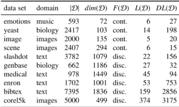
A total of 10 multi-label data sets are collected for experiments in this section, whose characteristics are summarized in Table 3. These data sets come from
different problem domains including text, biology, and
music. They can be found on the Mulan5 repository,
except for imagewhich comes from Zhou6 (Maron &
Ratan, 1998). LetDbe the multi-label data set, we use
|D|,dim(D),L(D),F(D) to represent the number of
ex-amples, number of features, number of possible labels,
and feature type respectively.DL(D)=|{Y|∃x: (x,Y)∈
D}|counts the number of distinct label combinations
ap-pearing in the data set. Continues values are binarized during the BN structure learning phase.
Table 3: Data sets characteristics
data set domain |D| dim(D) F(D) L(D) DL(D)
emotions music 593 72 cont. 6 27
yeast biology 2417 103 cont. 14 198
image images 2000 135 cont. 5 20
scene images 2407 294 cont. 6 15
slashdot text 3782 1079 disc. 22 156
genbase biology 662 1186 disc. 27 32
medical text 978 1449 disc. 45 94
enron text 1702 1001 disc. 53 753
bibtex text 7395 1836 disc. 159 2856
corel5k images 5000 499 disc. 374 3175
The performance of a multi-label classifier can be assessed by several evaluation measures (Tsoumakas
et al., 2010a). We focus on maximizing a
non-decomposable score function: the global accuracy (also
termed subset accuracy, complement of the 0/1-loss),
which measures the correct classification rate of the whole label set (exact match of all labels required).
4http://cran.r-project.org/web/packages/
randomForest
5http://mulan.sourceforge.net/datasets.html 6http://lamda.nju.edu.cn/data_MIMLimage.ashx
Note that the global accuracy implicitly takes into ac-count the label correlations. It is therefore a very strict evaluation measure as it requires an exact match of the predicted and the true set of labels. It was recently proved in (DembczyÅski et al., 2012) that BR is opti-mal for decomposable loss functions (e.g., the hamming loss), while non-decomposable loss functions (e.g. sub-set loss) inherently require the knowledge of the label conditional distribution. 10-fold cross-validation was performed for the evaluation of the MLC methods. 5.4.2. Results
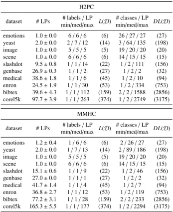
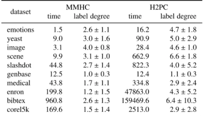
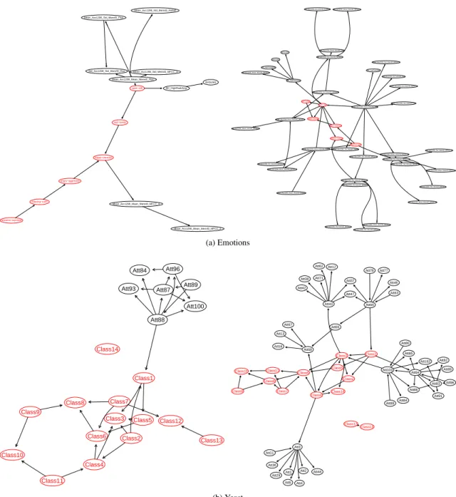
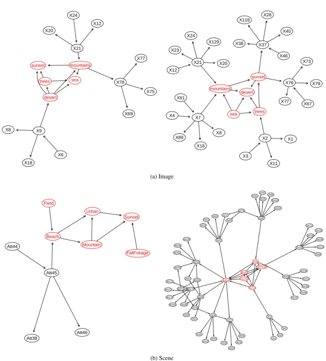
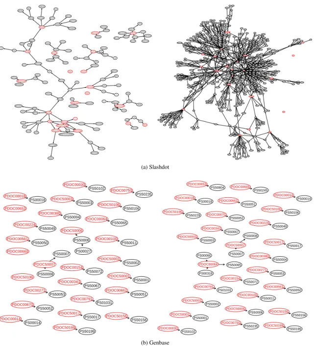
Table 4 reports the outputs of H2PC and MMHC, Ta-ble 5 shows the global accuracy of each method on the 10 data sets. Table 6 reports the running time and the average node degree of the labels in the DAGs obtained with both methods. Figures 3 up to 7 display graph-ically the local DAG structures around the labels, ob-tained with H2PC and MMHC, for illustration purposes. Several conclusions may be drawn from these exper-iments. First, we may observe by inspection of the av-erage degree of the label nodes in Table 6 that several
DAGs are densely connected, likesceneorbibtex, while
others are rather sparse, likegenbase, medical, corel5k.
The DAGs displayed in Figures 3 up to 7 lend them-selves to interpretation. They can be used for encod-ing as well as portrayencod-ing the conditional independen-cies, and the d-sep criterion can be used to read them
offthe graph. Many label powersets that are reported
in Table 4 can be identified by graphical inspection of the DAGs. For instance, the two label powersets in
yeast(Figure 3, bottom plot) are clearly noticeable in
both DAGs. Clearly, BNs have a number of advantages over alternative methods. They lay bare useful infor-mation about the label dependencies which is crucial if one is interested in gaining an understanding of the un-derlying domain. It is however well beyond the scope of this paper to delve deeper into the DAG interpreta-tion. Overall, it appears that the structures recovered by H2PC are significantly denser, compared to MMHC.
Onbibtexandenron, the increase of the average label
degree is the most spectacular. Onbibtex(resp.enron),
the average label degree has raised from 2.6 to 6.4 (resp. from 1.2 to 3.3). This result is in nice agreement with the experiments in the previous section, as H2PC was shown to consistently reduce the rate of false negative edges with respect to MMHC (at the cost of a slightly higher false discovery rate).
Second, Table 4 is very instructive as it reveals that
onemotions, image, and scene, the MLP approach boils
down to the LP scheme. This is easily seen as there is only one minimal label powerset extracted on average.
In contrast, on genbasethe MLP approach boils down
to the simple BR scheme. This is confirmed by inspect-ing Table 5: the performances of MMHC and H2PC (without feature selection) are equal. An interesting ob-servation upon looking at the distribution of the label powerset size shows that for the remaining data sets, the MLP mostly decomposes the label set in two parts: one on which it performs BR and the other one on which
it performs LP. Take for instanceenron, it can be seen
from Table 4 that there are approximately 23 label sin-gletons and a powerset of 30 labels with H2PC for a to-tal of 53 labels. The gain in performance with MLP over BR, our baseline learner, can be ascribed to the quality of the label powerset decomposition as BR is ignoring label dependencies. As expected, the results using MLP clearly dominate those obtained using BR on all data
sets except genbase. The DAGs display the minimum
label powersets and their relevant features.
Third, H2PC compares favorably to MMHC. On
scenefor instance, the accuracy of MLP+MB has raised
from 20% (with MMHC) to 56% (with H2PC). On
yeast, it has raised from 7% to 23%. Without feature
selection, the difference in global accuracy is less
pro-nounced but still in favor of H2PC. A Wilcoxon signed rank paired test reveals statistically significant improve-ments of H2PC over MMHC in the MLP approach
with-out feature selection (p<0.02). This trend is more
pro-nounced when the feature selection is used (p<0.001),
using MLP-MB. Note however that the LP
decompo-sition for H2PC and MMHC on yeast and image are
strictly identical, hence the same accuracy values in Ta-ble 5 in the MLP column.
Fourth, regarding the utility of the feature selection,
it is difficult to reach any conclusion. Whether BR or
MLP is used, the use of the selected features as inputs to the classification model is not shown greatly benefi-cial in terms of global accuracy on average. The per-formance of BR and our MLP with all the features out-performs that with the selected features in 6 data sets but the feature selection leads to actual improvements
in 3 data sets. The difference in accuracy with and
with-out the feature selection was not shown to be
statisti-cally significant (p>0.20 with a Wilcoxon signed rank
paired test). Surprisingly, the feature selection did
ex-ceptionally well ongenbase. On this data set, the
in-crease in accuracy is the most impressive: it raised from 7% to 98% which is atypical. The dramatic increase in
accuracy ongenbaseis due solely to the restricted
fea-ture set as input to the classification model. This is also
observed onmedical, to a lesser extent though.
Inter-estingly, on large and densely connected networks (e.g.
per-formed very well in terms of global accuracy and signif-icantly reduced the input space which is noticeable. On
emotions,yeast,image,sceneandgenbase, the method
reduced the feature set down to nearly 1/100 its
origi-nal size. The feature selection should be evaluated in
view of its effectiveness at balancing the increasing
er-ror and the decreasing computational burden by drasti-cally reducing the feature space. We should also keep in mind that the feature relevance cannot be defined in-dependently of the learner and the model-performance metric (e.g., the loss function used). Admittedly, our feature selection based on the Markov boundaries is not necessarily optimal for the base MLC learner used here, namely the Random Forest model.
As far as the overall running time performance is con-cerned, we see from Table 6 that for both methods, the running time grows somewhat exponentially with the size of the Markov boundary and the number of fea-tures, hence the considerable rise in total running time
onbibtex. H2PC takes almost 200 times longer on
bib-tex(1826 variables) andenron (1001 variables) which
is quite considerable but still affordable (44 hours of
single-CPU time onbibtexand 13 hours onenron). We
also observe that the size of the parent set with H2PC
is 2.5 (onbibtex) and 3.6 (onenron) times larger than
that of MMHC (which may hurt interpretability). In fact, the running time is known to increase exponen-tially with the parent set size of the true underlying net-work. This is mainly due the computational overhead of greedy search-and-score procedure with larger par-ent sets which is the most promising part to optimize in terms of computational gains as we discuss in the Con-clusion.
6. Discussion & practical applications
Our prime conclusion is that H2PC is a promising approach to constructing BN global or local structures around specific nodes of interest, with potentially thou-sands of variables. Concentrating on higher recall val-ues while keeping the false positive rate as low as
possi-ble pays offin terms of goodness of fit and structure
ac-curacy. Historically, the main practical difficulty in the
application of BN structure discovery approaches has been a lack of suitable computing resources and relevant accessible software. The number of variables which can be included in exact BN analysis is still limited. As a guide, this might be less than about 40 variables for ex-act structural search techniques (Perrier et al., 2008; Ko-jima et al., 2010). In contrast, constraint-based heuris-tics like the one presented in this study is capable of pro-cessing many thousands of features within hours on a
Table 4: Distribution of the number and the size of the minimal label powersets output by H2PC (top) and MMHC (bottom). On each data
set: mean number of powersets, minimum/median/maximum number
of labels per powerset, and minimum/median/maximum number of
distinct classes per powerset. The total number of labels and distinct labels combinations is recalled for convenience.
H2PC
dataset # LPs # labels/LP L(D) # classes/LP DL(D)
min/med/max min/med/max
emotions 1.0±0.0 6/6/6 (6) 26/27/27 (27) yeast 2.0±0.0 2/7/12 (14) 3/64/135 (198) image 1.0±0.0 5/5/5 (5) 19/20/20 (20) scene 1.0±0.0 6/6/6 (6) 14/15/15 (15) slashdot 9.5±0.8 1/1/14 (22) 1/2/111 (156) genbase 26.9±0.3 1/1/2 (27) 1/2/2 (32) medical 38.6±1.8 1/1/6 (45) 1/2/10 (94) enron 24.5±1.9 1/1/30 (53) 1/2/334 (753) bibtex 39.6±4.3 1/1/112 (159) 2/2/1588 (2856) corel5k 97.7±3.9 1/1/263 (374) 1/2/2749 (3175) MMHC
dataset # LPs min# labels/LP L(D) # classes/LP DL(D)
/med/max min/med/max
emotions 1.2±0.4 1/6/6 (6) 2/26/27 (27) yeast 2.0±0.0 1/7/13 (14) 2/89/186 (198) image 1.0±0.0 5/5/5 (5) 19/20/20 (20) scene 1.0±0.0 6/6/6 (6) 14/15/15 (15) slashdot 15.1±0.6 1/1/9 (22) 1/2/46 (156) genbase 27.0±0.0 1/1/1 (27) 1/2/2 (32) medical 41.7±1.4 1/1/4 (45) 1/2/7 (94) enron 36.8±2.7 1/1/12 (53) 1/2/119 (753) bibtex 77.2±3.1 1/1/28 (159) 2/2/233 (2856) corel5k 165.3±5.5 1/1/177 (374) 1/2/2294 (3175)
Table 5: Global classification accuracies using 4 learning methods
(BR, MLP, BR+MB, MLP+MB) based on the DAG obtained with
H2PC and MMHC. Best values between H2PC and MMHC are bold-faced. dataset BR MMHC H2PC MMHC H2PC MMHC H2PCMLP BR+MB MLP+MB emotions 0.327 0.371 0.391 0.147 0.266 0.189 0.285 yeast 0.169 0.273 0.271 0.062 0.155 0.073 0.233 image 0.342 0.504 0.504 0.227 0.252 0.308 0.360 scene 0.580 0.733 0.733 0.123 0.361 0.199 0.565 slashdot 0.355 0.419 0.474 0.274 0.373 0.278 0.439 genbase 0.069 0.069 0.069 0.974 0.976 0.974 0.976 medical 0.454 0.499 0.502 0.630 0.651 0.636 0.669 enron 0.134 0.165 0.180 0.024 0.079 0.079 0.157 bibtex 0.108 0.115 0.167 0.120 0.133 0.121 0.177 corel5k 0.002 0.030 0.043 0.000 0.002 0.010 0.034
Table 6: DAG learning time (in seconds) and average degree of the label nodes.
dataset time MMHClabel degree time H2PClabel degree
emotions 1.5 2.6±1.1 16.2 4.7±1.8 yeast 9.0 3.0±1.6 90.9 5.0±2.9 image 3.1 4.0±0.8 28.4 4.6±1.0 scene 9.9 3.1±1.0 662.9 6.6±1.8 slashdot 44.8 2.7±1.4 822.3 4.0±5.2 genbase 12.5 1.0±0.3 12.4 1.1±0.3 medical 43.8 1.7±1.1 334.8 2.9±2.4 enron 199.8 1.2±1.5 47863.0 4.3±5.2 bibtex 960.8 2.6±1.3 159469.6 6.4±10.3 corel5k 169.6 1.5±1.4 2513.0 2.9±2.8
personal computer, while maintaining a very high struc-tural accuracy. H2PC and MMHC could potentially handle up to 10,000 labels in a few days of single-CPU time and far less by parallelizing the skeleton identifica-tion algorithm as discussed in (Tsamardinos et al., 2006; Villanueva & Maciel, 2014).
The advantages in terms of structure accuracy and its ability to scale to thousands of variables opens up many avenues of future possible applications of H2PC in var-ious domains as we shall discuss next. For example, BNs have especially proven to be useful abstractions in computational biology (Nagarajan et al., 2013; Scutari & Nagarajan, 2013; Prestat et al., 2013; Aussem et al., 2012, 2010; Pe˜na, 2008; Pe˜na et al., 2005). Identify-ing the gene network is crucial for understandIdentify-ing the behavior of the cell which, in turn, can lead to better di-agnosis and treatment of diseases. This is also of great importance for characterizing the function of genes and the proteins they encode in determining traits, psychol-ogy, or development of an organism. Genome sequenc-ing uses high-throughput techniques like DNA microar-rays, proteomics, metabolomics and mutation analysis to describe the function and interactions of thousands of genes (Zhang & Zhou., 2006). Learning BN models
of gene networks from these huge data is still a difficult
task (Badea, 2004; Bernard & Hartemink, 2005; Fried-man et al., 1999a; Ott et al., 2004; Peer et al., 2001). In these studies, the authors had decide in advance which genes were included in the learning process, in all the cases less than 1000, and which genes were excluded from it (Pe˜na, 2008). H2PC overcome the problem by focusing the search around a targeted gene: the key step
is the identification of the vicinity of a nodeX (Pe˜na
et al., 2005).
Our second objective in this study was to demonstrate the potential utility of hybrid BN structure discovery to multi-label learning. In multi-label data where many
inter-dependencies between the labels may be present, explicitly modeling all relationships between the labels is intuitively far more reasonable (as demonstrated in our experiments). BNs explicitly account for such inter-dependencies and the DAG allows us to identify an op-timal set of predictors for every label powerset. The ex-periments presented here support the conclusion that lo-cal structural learning in the form of lolo-cal neighborhood induction and Markov blanket is a theoretically well-motivated approach that can serve as a powerful learn-ing framework for label dependency analysis geared toward multi-label learning. Multi-label scenarios are found in many application domains, such as multimedia annotation (Snoek et al., 2006; Trohidis et al., 2008), tag recommendation, text categorization (McCallum, 1999; Zhang & Zhou., 2006), protein function classification (Roth & Fischer, 2007), and antiretroviral drug catego-rization (Borchani et al., 2013).
7. Conclusion & avenues for future research We first discussed a hybrid algorithm for global or local (around target nodes) BN structure learn-ing called Hybrid HPC (H2PC). Our extensive experi-ments showed that H2PC outperforms the state-of-the-art MMHC by a significant margin in terms of edge recall without sacrificing the number of extra edges, which is crucial for the soundness of the super-structure used during the second stage of hybrid methods, like the ones proposed in (Perrier et al., 2008; Kojima et al., 2010). The code of H2PC is open-source and
publicly available online at https://github.com/
madbix/bnlearn-clone-3.4. Second, we discussed
an application of H2PC to the multi-label learning prob-lem which is a challenging probprob-lem in many real-world application domains. We established theoretical results, under the faithfulness condition, in order to characterize graphically the so-called minimal label powersets that appear as irreducible factors in the joint distribution and their respective Markov boundaries. As far as we know, this is the first investigation of Markov boundary
princi-ples to the optimal variable/feature selection problem in
multi-label learning. These formal results offer a simple
guideline to characterize graphically : i) the minimal la-bel powerset decomposition, (i.e. into minimal subsets
YLP ⊆ Ysuch that YLP ⊥⊥ Y\YLP | X), and ii) the
minimal subset of features, w.r.t an Information Theory criterion, needed to predict each label powerset, thereby reducing the input space and the computational burden of the multi-label classification. The theoretical analysis laid the foundation for a practical multi-label classifica-tion procedure. Another set of experiments were carried