GIS and Predictive Modeling: a Comparison of Methods Applied to Schima superba Potential Habitat and Decision Making

GIS and Predictive Modeling: a Comparison of Methods Applied to

Schima superba Potential Habitat and Decision Making

Hou-Chang Chen1 Nan-Jang Lo2 Wei-I Chang3Kai-Yi Huang4

1

Undergraduate (Senior), Dept. of Forestry; 2Specialist, Experimental Forest Management Office; 3Chief, Forest Planning Section, Forest Bureau, Council of Agriculture, Taipei 100,

Taiwan; 4Professor, Dept. of Forestry, Chung-Hsing University, 250 Kuo-Kuang Road, Taichung 402, Taiwan. Tel: +886-4-2854663; Fax: +886-4-22854663

E-mail: [email protected]; [email protected]; [email protected]; [email protected] (Corresponding author’s e-mail)

KEY WORDS: Geographic Information System (GIS), Decision Tree (DT), Logistic Multiple Regression (LMR), Discriminant Analysis (DA), Potential Habitat.

ABSTRACT Recently, in order to alleviate the impact of environmental issues due to global warming, forestation, which may increase forest cover and thus enhance the quantity of carbon sequestration, has become one of the most effective measures for carbon reduction. However, most of the previous plantations could not have achieved the goal of carbon reduction, since they did not follow the principle of “planting the right tree at right place”. We attempted to predict the potential habitat for planting Chinese guger-tree (Schima superba) in the Huisun study area in central Taiwan. We applied GIS to overlay the tree samples collected with GPS on the layers of elevation, slope, aspect, terrain position, and vegetation indices derived from SPOT-5 images for modeling the tree’s habitat. We developed decision tree (DT), logistic multiple regression (LMR) and discriminant analysis (DA) models to predict the tree’s potential sites in Huisun. Results based on the tree samples from Tong-Feng watershed in Huisun indicated that the accuracy of DT was slightly better than that of LMR, accuracies of the two models were much better than that of DA; and the three models were highly efficient in habitat modeling. DT and LMR models greatly reduced the area of field survey to less than 10% of the entire study area at the first stage, they were better suited for potential habitat modeling. Vegetation indices may not be useful for improving model accuracy for the widely distributed species. However, the reasons are still waiting to be further assessment.

1. INTRODUCTION

Global warming and climate change issues have been drastically debated around the world. Facing the issues, the government has proposed afforestation policy for enhancing carbon sinks. However, the past afforestation projects almost resulted in low survival rate and low growth rate with planted trees, and couldn’t achieve the aim of mitigating carbon emissions. The reason was that plantation didn’t meet the principle of “the right tree for the right place”. We wanted to use 3S technologies combining remote sensing, geographic information system, and global positioning system to establish a standard operating procedure (SOP). The SOP that would apply to model suitable habitats of various species will provide as a reference of species and plantations selection when planting operations to improve effectiveness of forestation.

Images from remote sensing have been widely applied in the land-cover and land-use classification of. However, application of vegetation classification was still difficult because the spectral reflectance differences of plants were more subtle, especially in the forest with higher complexity. Mundt et al. (2006) used airborne hyperspectral images and LiDAR data to classify effectively distributions of sagebrush vegetation in Idaho National Engineering and Environmental Laboratory (INEEL) in U.S. Suhaili et al. (2007) also used airborne hyperspectral data on classification and mapping in tropical forest in Kepong, Malaysia. Landenburger et al. (2008) used a combination of classification tree analysis method, Landsat 7

ETM+ satellite images, and extensive stand data to map distributions of whitebark pines that grow in the Greater Yellowstone Ecosystem in the U. S. A.

Chinese guger-tree (Schima superba.) species, widely distributed from 300 m to 2,300 m in Taiwan, is one of the fine broad-leaf tree species and good for fitment. Chinese guger-trees (CGT) have high water content and dense crown closure, and high dispersal ability; therefore, they have excellent fire resistance characteristics and can grow to form a fire line (Luo et al., 2005). In the past, a limited number of studies have applied GIS to wide distribution vegetation. We chose CGT as a target for the study to evaluate the applicability of GIS.

We used GIS to overlay tree samples collected with GPS on the layers of vegetation indices derived from SPOT-5 images, elevation, slope, aspect, and terrain position to analyze its spatial distribution. Decision tree (DT), logistic multiple regression (LMR) and discriminant analysis (DA) models were developed to predict its potential habitat. The objective of this study was to evaluate the effect of vegetation indices on model accuracy and to select a best model by comparing accuracies and efficiency of three models of modeling suitable habitat.

2. STUDY AREA

The study area cover the Huisun Forest Station, the property of Chung-Hsing University, in central Taiwan, situated within 24°2´–24°5´ N latitude and 121°3´–121°7´ E longitude. The station has a total area of 7,477 ha. The altitude ranges from 454 m to 2,419 m, and its climate is temperate and humid. Hence, the study area has nourished many different plant species and is a representative forest in central Taiwan. It comprises five watersheds, including two larger Kuan-Dau watershed at west and the Tong-Feng watershed at east, and all of the tree samples (ground data) were collected from the Tong-Feng watershed by using a GPS.

3. MATERIALS AND METHODS 3.1 Data Collection

Digital elevation model (DEM) with grid size 5  5 m, orthophoto base map (1:10,000), and nine-date SPOT-5 images were collected. Two-date SPOT-5 images (10/07/2004 and 11/11/2005) were selected because the two-date images have the best quality with the least amount of clouds. In-situ data (Chinese guger-tree samples) were also acquired by using a GPS linked with a laser range.

3.2 Data Processing

Slope and aspect data layers were generated from 5  5 m DEM by using ERDAS Imagine software module. The ridges and valleys in the study area interpreted from the contour lines shown on the orthophoto base maps were used together with DEM to generate terrain position layer. These lines were then digitized to establish the data layer of main ridges and valleys by using ARC/INFO software for later use. The data layer of main ridges and valleys in a vector format was converted into a new data layer in a raster format by ERDAS Imagine software, and then combined with DEM to generate terrain position layer (Skidmore, 1990). Vegetation indices were derived from the two-date SPOT-5 images, one in autumn, the other in summer, by using Spatial Modeler of ERDAS Imagine. The moisture content within different plant’s leaves would have different change between dry season (autumn) and wet season (summer), we use the difference ratio of near and mid infrared of two SPOT-5 images to discriminate plants with different change of moisture content. Chinese guger-tree samples obtained by GPS were converted into ArcView shapefile format for later use. There were 122 samples collected in the study, and 82 tree samples were used for model development (training) and the remaining, 40 tree samples, were used for model validation (test) in this study.

3.3 Database Building and Sampling

The GIS database used in the study was constructed by using ERDAS Imagine software module Layer Stack to make elevation, slope, aspect, terrain position, and vegetation index layers overlaid. The Chinese guger-tree sample layer was overlaid with five data layers, and those pixels of the five layers lying at the same position with tree sample pixels were clipped out. Because non-target sites (background) correspond to the vast majority of the study area, larger variation is expected in environmental characteristics for this group. The number of non-target pixels (sites) should be three times more than that of target pixels to increase the probability of acquiring a more representative sample of the habitat characteristics at non-target sites (Pereira and Itami 1991, Sperduto and Congalton 1996), and the sample data for non-target groups (background) were taken from data layers by the random sampling technique to minimize spatial autocorrelation in the independent variables (Pereira and Itami, 1991).

3.4 Model Development

The predictive models for selecting potential habitat of the trees were created using three statistical methods: (1) decision trees, (2) logistic multiple regression, and (3) discriminant analysis. Model development and validation can be done by cross-validation (it is called split-sample validation). Split-sample validation can be implemented by dividing a dataset into two subsets, the first one (training dataset) typically comprising one-half to two-thirds of all data and the other (test dataset) comprising one-third to one-half of all data. The first one is used to build and test a model. The other one (an independent dataset) is just used to test the model, not used to build the model. Three models were implemented by using SPSS software package in the study.

3.4.1 Decision Tree

Decision trees are a sequential partitioning of the dataset in order to maximize differences on a dependent variable. Decision pathways originate from a starting node (root) that contains all observations and end at multiple nodes containing unique subsets of observations. Terminal nodes are assigned a final outcome based on group membership of the majority of observations (De’ath and Fabricius, 2000; Bourg et al., 2005; O’Brien et al., 2005).

3.4.2 Logistic Multiple Regression

The LMR model developed in the study can be expressed as follows:









where P is the probability potential habitat of the tree species at a particular position, Yh is

dependent variable, x1, … , xn are a set of independent predictor (biophysical) variables, and

B0, . . ., Bn are logistic coefficients. The output probability values range from 0 to 1, with 0

indicating absence (a 0 percent probability of the target habitat) and 1 indicating presence (a 100 percent probability). The default threshold of 0.5 implies that probabilities above 0.5 are target habitat and below 0.5 are non-target habitat (Gross et al., 2002; O’Brien et al., 2005).

3.4.3 Discriminant Analysis

Discriminant analysis is a technique, which discriminates among k classes (objects) based on a set of independent or predictor variables. The objectives of DA are to (1) find linear composites of n independent variables which maximize among-groups to within-groups variability; (2) test if the group centroids of the k dependent classes are different; (3) determine

which of the n independent variables contribute significantly to class discrimination; and (4) assign unclassified or “new” observations to one of k classes (Lowell, 1991). The variates for a discriminant analysis, also known as the discriminant function takes the following form:

Z j k = a + W1X1 k + W2 X 2 k + . . . + W n X n k (2)

where

Z j k = discriminant Z score of discriminant function j for object (class) k

a = intercept

Wi = discriminant weight for independent variable i

X i k = independent variable i object (class) k

3.5 Model Validation

Model validation can be done by cross-validation (split-sample validation). Split-sample validation can be implemented by dividing a dataset into two subsets, the first one typically comprising one-half to two-thirds of all data and the other comprising one-third to one-half of all data. The first one (training dataset) is used to build and test a model; the other one (test dataset) is used to validate the model. For each model, predict the response of the remaining data, and calculate the error from the predictions and the observed values (De’ath and Fabricius, 2000).

4. RESULTS AND DISCUSSION

Table 1 summarizes basic statistics of five predictor variables for the entire study area and CGT sites. The table shows that CGTs grow at higher altitude more than 1,000m in the study area and also indicate that they may only grow at areas with higher altitude, and we really did not found it at areas with lower altitude in field survey. Furthermore, slope and TP statistics with CGT sites show that most CGTs prefer to grow at gentler slopes and near-ridge positions.

Table 1 Basic statistics of five predictor variables for the entire study area and CGT sites.

Statistics Entire Area CGT Altitude (m) Slope () Aspect () TP VI Altitude (m) Slope () Aspect () TP VI Mean 1314 34 185 5 24 1812 20 201 7 23 Mode 1239 37 127 5 22 1824 15 254 7 22 Maximum 2418 89 361 8 119 2054 40 353 8 31 Minimum 445 0 0 1 0 1225 1 10 5 20 TP = Terrain Position; VI = Vegetation Index

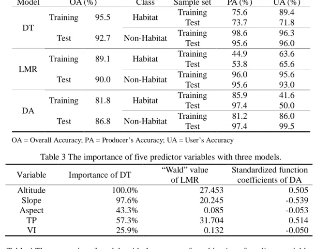
Table 2 shows the accuracies of three models with three predictor variables (altitude, slope, and terrain position) for predicting potential habitat of CGT. The accuracy of the DT model is slightly higher than that of the LMR model, and both of the two models are significantly better than that of the DA model, both in training and test cases. Moreover, the user’s accuracies of habitat with DT (average about 80%) are higher than those of LMR (average about 64%), and the user’s accuracies of habitat with DT and LMR are much higher than those of DA (average about 45%). The three models can be implemented efficiently using SPSS and ERDAS Imagine software package, thereby saving much labor and time. Of more importance is that the use of predictive models can greatly reduce the amount of fieldwork required for forestry-related studies.

Table 2 The accuracies of three models with predictor variables altitude, slope, and TP. Model OA (%) Class Sample set PA (%) UA (%)

DT

Training 95.5 Habitat Training 75.6 89.4 Test 73.7 71.8 Test 92.7 Non-Habitat Training 98.6 96.3 Test 95.6 96.0

LMR

Training 89.1 Habitat Training 44.9 63.6 Test 53.8 65.6 Test 90.0 Non-Habitat Training 96.0 95.6 Test 95.6 93.0

DA

Training 81.8 Habitat Training 85.9 41.6 Test 97.4 50.0 Test 86.8 Non-Habitat Training 81.2 86.0 Test 97.4 99.5

OA = Overall Accuracy; PA = Producer’s Accuracy; UA = User’s Accuracy

Table 3 The importance of five predictor variables with three models.

Variable Importance of DT “Wald” value of LMR Standardized function coefficients of DA Altitude 100.0% 27.453 0.505 Slope 97.6% 20.245 -0.539 Aspect 43.3% 0.085 -0.053 TP 57.3% 31.704 0.514 VI 25.9% 0.132 -0.050

Table 4 The accuracies of models with three types of combination of predictor variables.

Combination

Overall Accuracy (%)

DT LMR DA

Training Test Training Test Training Test B1, B2, B4 95.5 92.7 89.1 90.0 81.8 86.8 B1, B2, B4, B3 96.9 94.1 88.8 90.0 81.8 87.5 B1, B2, B4, B5 95.8 93.8 88.9 90.0 81.5 86.5

B1 = Altitude; B2 = Slope; B3 = Aspect; B4 = Terrain Position; B5 = Vegetation Index

Table 3 shows the relative importance of five predictor variables with three predictive models for predicting the potential habitat of CGTs. According to the importance ratios from DT implementation, altitude and slope contributed more significantly to class discrimination, followed by TP (B4), while aspect (B3) and vegetation index (B5) contributed the least. The Wald statistics derived from LMR implementation and standardized function coefficients from DA implementation also showed the same result as mentioned above. The models built from three variables (altitude, slope, and TP) were used as basis and compared with the same models but with one more variable, VI (vegetation index derived from SPOT-5 images), as shown in table 4. Results show that VI improved the model performance insignificantly in all three models. This is because the spectral resolution and spatial resolution of SPOT-5 imagery are not enough to discriminate CGT from other plants.

5. CONCLUSIONS

The study developed the three models of DT, LMR, and DA to extrapolate the tree’s potential sites in the study area. The accuracy of the DT model is slightly higher than that of

the LMR, and both of first two are much higher than that of the DA; the three models can be implemented efficiently in modeling the potential habitat. Therefore, the DT and LMR models are better suited for predicting the tree’s potential habitat. The results also have shown that the vegetation indices derived from SPOT-5 satellite images may not be able to significantly improve model accuracy due to the limits of their spectral resolutions with SPOT-5 imagery not enough to discriminate the slight difference of the electromagnetic spectrum reflected among the varieties of trees and spatial resolutions not enough to discriminate the dispersedly distributed tree species. Airborne hyperspectral data and LIDAR data will be used in follow-up studies so that the model accuracy can be improved. Finally, the tree samples in this study were acquired only from the Tong-Feng watershed, we will add more samples acquired from the Kuan-Dau watershed into the models to verify the reliability of the models.

6. REFERENCES

Bourg, N. A., W. J. Mcshea and D. E. Gill, 2005. Putting a CART before search: successful habitat prediction for a rare forest herb. Ecology, 86 (10), pp. 2793–2804.

De’ath, G. and K. E. Fabricius, 2000. Classification and regression trees: a powerful yet simple technique for ecological data analysis. Ecology, 81 (11), pp. 3178–3192.

Gross, J. E., M. C. Kneeland, D. F. Reed, and R. M. Reich, 2002. GIS-based habitat models for mountain goats. Journal of Mammalogy, 83 (1), pp. 218–228.

Landenburger, L., R. L. Lawrence, S. Podruzny, and C. C. Schwartz, 2008. Mapping regional distribution of a single tree species: white bark pine in the Greater Yellowstone Ecosystem. Sensors, 8, pp. 4983–4994.

Lowell, K., 1991. Utilizing discriminant function analysis with a geographical information system to model ecological succession spatially. International Journal of Geographical Information System, 5 (2), pp.175–191.

Luo, Y., X. N. Zeng, J. H. Ju, S. Zhang, S. Z. Wu, 2005. Molluscidal activity of the methanol extracts of 40 species of plants. Plant Protect, 31, pp.31–34. (In Chinese)

Mundt, J. T., D. R. Streutker, and N. F. Glenn, 2006. Mapping sagebrush distribution using fusion of hyperspectral and lidar classifications. Photogrammetric Engineering & Remote Sensing, 72 (1), pp. 47–54.

O’Brien, C. S. S. Rosenstock, J. J. Hervert, J. L. Bright, and S. R. Boe, 2005. Landscape – level models of potential habitat for Sonoran pronghorn. Wildlife Society Bulletin, 33 (1), pp. 24–34.

Pereira, J. M. C., and R. M. Itami, 1991. GIS-based habitat modeling using logistic multiple regression: a study of the Mt. Graham red squirrel. Photogrammetric Engineering & Remote Sensing, 57 (11), pp.1475–1486.

Skidmore, A. K., 1990. Terrain position as mapped from a grided digital elevation model. Int. J. of Geographical Information Systems, 4 (1), pp. 33–49.

Sperduto, M. B., and R. G. Congalton, 1996. Predicting rare orchid (small Whorled Pogonia) habitat using GIS. Photogrammetric Engineering & Remote Sensing, 62 (11), pp.1269–1279.

Suhaili, A., N. A. Ainuddin, A. G. Awang Noor, I. Faridah Hanum, and H. Z. M. Shafri, 2007. Application of airborne hyperspectral sensing for tropical forest mapping. Asian Conference on Remote Sensing 2007, Nov 12-16, Kuala Lumpur, Malaysia, TS 39.3.