using Local Optima Networks
Jonathan E. Fieldsend
University of Exeter Department of Computer Science
Khulood Alyahya
University of Exeter Department of Computer Science
ABSTRACT
Local optima networks (LONs) represent the landscape of optimi-sation problems. In a LON, graph vertices represent local optima in the search domain, their radii the basin sizes, and directed edges between vertices the ability to transit from one basin to another (with the edge width denoting how easy this is). Recently, a network construction approach inspired by LONs has been proposed for multi-objective problems which uses an undirected graph, repre-senting mutually non-dominating solutions and neighbouring links, but not basin sizes. In contrast, here we introduce two formulations for multi/many-objective problems which are analogous to the tra-ditional LON, using dominance-based hill-climbing to characterise the search domain. Each vertex represents a set of locally optimal solutions, with basins and ease of transition between them shown. These LONs vary depending on whether a point-based (dominance neutral optima) or set-based (Pareto local optima) representation is used to define mode construction. We illustrate these alternative formulations on some illustrative problems. We discuss some of the underlying computational issues in constructing LONs in a multi-objective as opposed to uni-multi-objective problem domain, along with the inherent issue of neutrality — as each a vertex in these graphs almost invariably represents a set in our proposed constructs.
CCS CONCEPTS
•Mathematics of computing→Combinatorial optimization;
Graph theory; •Applied computing→Multi-criterion
opti-mization and decision-making; •Human-centered
comput-ing→Visualization;Visualization design and evaluation
meth-ods;
KEYWORDS
multi-objective optimisation; fitness landscapes
ACM Reference Format:
Jonathan E. Fieldsend and Khulood Alyahya. 2019. Visualising the Landscape of Multi-Objective Problems using Local Optima Networks. InGenetic and
Evolutionary Computation Conference Companion (GECCO ’19 Companion),
Permission to make digital or hard copies of all or part of this work for personal or classroom use is granted without fee provided that copies are not made or distributed for profit or commercial advantage and that copies bear this notice and the full citation on the first page. Copyrights for components of this work owned by others than the author(s) must be honored. Abstracting with credit is permitted. To copy otherwise, or republish, to post on servers or to redistribute to lists, requires prior specific permission and /or a fee. Request permissions from [email protected].
GECCO ’19 Companion, July 13–17, 2019, Prague, Czech Republic
© 2019 Copyright held by the owner/author(s). Publication rights licensed to the Association for Computing Machinery.
ACM ISBN 978-1-4503-6748-6/19/07. . . $15.00 https://doi.org/10.1145/3319619.3326838
July 13–17, 2019, Prague, Czech Republic.ACM, New York, NY, USA, 9 pages. https://doi.org/10.1145/3319619.3326838
1
INTRODUCTION
Local optima networks (LONs) have been developed and used to visualise the landscape of uni-objective problems [12, 17], using directed graphs with variable node size and colour to denote infor-mation about the search landscape. Recent work inspired by LONs has proposed a network representation for multi-objective problems [10]. These Pareto local optimal solutions networks (PLOS-nets) use undirected graphs. Each vertex representing a single local optima, with edges connecting neighbouring solutions. In contrast with PLOS-nets, we present here definitions of LONs for multi-objective problems which employ directed graphs, convey information re-garding basin sizes and which can incorporate the standard edge definitions used in LONs. Due to the nature of multi-modality in multi-objective problems, the vertices represent sets of solutions rather than single solutions in our approach. As such, to the best of the authors’ knowledge, this work presents the first full trans-ference of the LON landscape visualisation methodology to the multi-objective domain.
We present two formulations: one relying on a point-based hill-climb anddominanceto describe contiguous regions of neutrality under this measure to define vertices, the other, relying on a set-based search approach, which results in vertices composed of Pareto local optima.
The paper proceeds as follows: Section 2 briefly describes local optima networks, as developed in the uni-objective optimisation domain; Section 3 describes the multi/many-objective optimisa-tion problem, along with the different types of optima that inhabit this landscape, and how they are identified; Section 4 describes the PLOS-net of [10] before introducing our two new LON-based approaches along with bi-objective examples; Section 5 provides illustrations of the proposed LONs constructs on some larger many-objective problems. The paper concludes with a discussion in Sec-tion 6.
2
LOCAL OPTIMA NETWORKS
A LON is a network-based model that compresses the information of the search space into a weighted oriented graph. The model is adapted from the inherent networks of energy landscapes in physical-chemistry and is used as a method to visualise and ap-ply complex network analysis tools to combinatorial optimisation problems [12, 17]. The vertices of a given landscape graph are the local optima under its neighborhood operator. An edge between two vertices can be defined in different ways. It was originally de-fined in such a way to represent when two optima have adjacent
Algorithm 1Greedy (best) improvement hill-climbing
Require: xst ar t ▷Initial sample
1: xend :=xst ar t 2: converдed:=false
3: whileconverдed=falsedo 4: better_f ound:=false 5: forx′∈N(xend)do
6: iff(x)<f(xend)then ▷If neighbour is better 7: xend =x ▷Replace with better neighbour 8: better_f ound:=true
9: end if
10: end for
11: ifbetter_f ound=truethen
12: goto4 ▷Better neighbour found, so climb again 13: else
14: converдed:=true ▷No better neighbour found 15: end if
16: end while
17: returnxend ▷Return path start and end locations
Algorithm 2First improvement hill-climbing
Require: xst ar t ▷Initial sample
1: xend :=xst ar t 2: converдed:=false
3: whileconverдed=falsedo
4: Z:=random_order(N(xend))▷Random order neighbours 5: forz∈Zdo ▷For each randomly ordered neighbour 6: iff(z)<f(xend)then ▷If neighbour is better 7: xend =z ▷Replace with better neighbour 8: goto4 ▷Better neighbour found, so climb again
9: end if
10: end for
11: converдed:=true ▷No better neighbour found 12: end while
13: returnxend ▷Return path start and end locations
basins (i.e. the transition probability between the basins of the two optima). However, this definition was found to be computationally expensive and produces a densely connected graph. An alterna-tive definition of an edge was therefore proposed to represent the probability of escaping from one local optimum to another after applying controlled mutation followed by hill-climbing [18].
Local optima networks have been applied to study the landscape of several combinatorial optimisation problems, e.g. [2, 6, 13]. It has also been applied to study the behaviour of different local search methods. For example, in [14] LONs are applied toN K problem examples with two different hill-climbing algorithms employed to generate paths, and hence define the subsequent LONs generated. These were (i) the greedy hill-climbing formulation used in ear-lier work on LONs, which always selects the best move out of all neighbours (detailed in Algorithm 1), and (ii) the next improve-ment hill-climbing formulation which selects the first evaluated of the neighbours (randomly ordered) that is better than the cur-rent design (detailed in Algorithm 2). LONs generated using these
two different algorithms were designated b-LONs and f-LONs re-spectively. The edges were calculated using the basin transition definition. Calculating the f-LONs is obviously cheaper compared to b-LONs where each move requires the evaluation of the entire neighbourhood. The f-LONs were found to be more dense than b-LONs with lower weighted self-loops indicating that it is easier to escape an optimum using first-improvement hill-climber. The shortest paths in f-LONs were found to be on average slightly longer than the ones in b-LONs.
Most of the existing work on LONs were limited to relatively small problem sizes due to the requirement of complete enumera-tion of the search space to find all local optima and calculate the edges between them. However, recently sampling methods have been proposed to sample LONs efficiently [3] and in statistical sound way as not to lose accuracy of the network metrics [19]. Other methods have been proposed to sample LONs from the ac-tual runs of local search methods [7, 11].
The LON construction for uni-objective landscapes exhibiting neutrality was investigated in [21] on neutral variants ofNK land-scapes. The study generated LONs using exact calculation and thus was limited to enumerable problem sizes. The main issue they found with neutrality is the definition of basins of attraction and the transition between them. LONs were defined such that each vertex represents a network of neutral neighbours, i.e. a plateau. An edge between two vertices was defined as the transition probability between their basins of attraction. In [19], they mention as future work extending their sampling method to sample LONs of fitness landscapes with significant neutrality.
3
MULTI-OBJECTIVE OPTIMISATION
In the general multi-objective optimisation case (two or three ob-jectives) and the many-objective optimisation case (four or more objectives) we seek to find the Pareto set of solutions — or, more realistically, an estimate of it. Without loss of generality, we seek to simultaneously minimiseKobjectives:fk(x),k=1, . . . ,K, where each objective depends upon a vectorx=(x1, . . . ,xN)ofNdesign or decision variables. These variables may be continuous, discrete, or a combination of both. The variables may also be subject to equality and inequality constraints. Such constraints defineX: the feasible design space.
When there is more than one objective to be minimised, solu-tions may exist for which performance on one objective cannot be improved without reducing performance on at least one other. Such solutions are said to bePareto optimal. The set of all Pareto optimal solutions is said to form thePareto set, whose image in the objective space is known as thePareto front. Identifying such solutions relies on Paretodominance. A decision vectorxis said to dominate anotherx′iff
fk(x) ≤fk(x′) for all k=1, . . . ,K and f(x),f(x′). (1)
This is often simply denoted asx ≺x′rather thanf(x) ≺f(x′). Formally, the Pareto set (the global Pareto optima, or GPO) can be extracted fromXusing thenondomfunction:
Algorithm 3Pareto Local Search (PLS) of [15].
Require: xst ar t ▷Initial sample
1: F:={xst ar t} ▷Initial set to process 2: XP LO :=∅ ▷Set holding estimated PLO 3: whileF,∅do ▷While still locations to process 4: x:=random_draw(F)
5: W:=∅
6: for allx′∈ N (x)do
7: ifx′′∈W∪F∪XP LO|x′′⪯x′then
8: W :=W∪x′▷Not dominated by current estimate
9: end if 10: end for 11: XP LO:={x′|x′∈XP LO:x′′∈W|x′′≺x′} 12: F:=F\ {x} ∪W 13: F:={x′|x′∈F:x′′∈W|x′′≺x′} 14: end while
15: returnXP LO ▷Return path start location and end set
however in practice|X|is often too large to be exhaustively searched, and optimisers seek to return an approximation toXG P O(the set returned by nondom(X)), in terms of quality underf.
What does a fitness landscape mean in the context of multi- or many-objective optimisation? Multi-objective optimisation is most typically a set-based procedure. Even single parent single child (1+1) methods like the popular PAES algorithm [9] rely on maintaining an archive of the approximated Pareto set, to reference for movement decisions. WhenXis in the plane we may use dominance landscapes [4] to visualise the local search landscape, however in higher design dimensions it is natural to explore whether there is an appropriate analogue of the uni-objective LON visualisation. To do this we need to consider what the multi-objective equivalent to the point-based hill-climbing used in LONs is.
3.1
Pareto local optima
We first consider theset-basedlocal hill-climb described in Pareto Local Search (PLS) [15]. This is detailed in Algorithm 3. Although it starts with a single point in design space, it maintains a dy-namic set to identify the Pareto local set of solutions (the Pareto local optima) identified from hill-climbing from an initial point. This set is comprised entirely of mutually non-dominating designs. More formally, the Pareto local optimum (PLO) setXP LO ∈ X with respect to the neighbour functionNis composed such that
∀x ∈ XP LOx′ ∈ N (XP LO)wherex′ ≺x(see e.g. [15, 20] for further details).
Consider the simple problem illustrated in Figure 1, using the von Neumann neighbourhood function in a box constrained plane. Here there are two criteria evaluated on designs from the domain
X, which has 25 members in total. There are two distinct spatial groupings ofXP LOindividuals, which are shown with red vertices. The Pareto set (the global Pareto optima) are highlighted with blue circles, and are a subset of the union of all PLO.
Figure 2 illustrates the process from an initial sample to conver-gence using PLS on the problem from Figure 1. Outwardly using PLS to characterise the landscape is an attractive approach, how-ever, from a practical point of view (and as identified in [15]) it can
9,9 9,9 9,9 8,8 7,7 9,9 8,7 7,7 7,6 5,7 8,8 9,8 8,8 6,7 6,3 8,8 8,7 7,7 4,5 5,4 4,4 5,4 3,7 3,6 7,2
Figure 1: Landscape illustration. Each vertex represents a so-lution, with edges connecting neighbours underN. Cost un-der two criteria denoted to the top right of a vertex.XP LO
members are coloured red. The global Pareto optima (GPO) are circled in blue. Note in this exampleXG P O,ÐiXP LOi .
t=0 t=1 t=2
t=3 t=4 t=5
t=6 t =7
Figure 2: Landscape hill-climb illustration using PLS on the problem shown in Figure 1, with repetitionst of the while loop. The start point is denoted with a green node, the esti-mate ofXP LOwith red nodes, andN (XP LO) \XP LOwith grey
nodes.
be prohibitively expensive in large domains. This is because, where a landscape is approximated with a fixed budget rather than com-pletely enumerated, one may spend the entire budget on a single hill-climb (and resultant local Pareto set enumeration), rather than approximating the landscape over the broader domain. Effectively, eachXP LObehaves similarly to a plateau in the uni-objective fit-ness landscape. However, this landscape feature is considerably more expensive to identify and explore. In the uni-objective case, a solution equal in fitness to one plateau member is equal in fit-ness to all other members, but in the multi-objective case being
10,10 9,9 9,9 9,9 9,9 9,9 1,9 5,3 5,6 6,5 10,10 9,9 5,2 4,2 2,4 11,11 11,12 10,7 5,3 3,5 2,3 13,15 9,8 6,7 6,6
Figure 3: Landscape illustration. Each vertex represents a so-lution, with edges connecting neighbours underN. Cost un-der two criteria denoted to the top right of a vertex. There are threeXP LO, whose members are coloured red. However,
depending on the start location two of theXiP LOwill be re-turned as asingleset from a hill-climb. The global Pareto optima (GPO) are circled in blue.
mutually non-dominated with one local Pareto set memberdoes not ensure mutual non-domination with all other members of anXi
P LO. Although the use of advanced data structures means the compu-tational cost of comparison does not need to grow linearly with the set size [5, 8], nevertheless, the computational cost of verifying membership still grows with|Xi
P LO|, and can become a significant computational burden.
3.1.1 Inconsistency of landscape under Pareto local search, and
implications.Until now we have denoted the distinct PLO sets
returned by an initial location in PLS asXi
P LO. However, a property not generally discussed in the literature regarding the PLO returned from PLS is that in some cases bothXi
P LO∩X j
P LO,∅andXP LOi \
Xj
P LO,∅are true. The root cause of this that the PLO returned by PLS can bedisjoint. That is, one or more elements of the returned set are not reachable by walking from other members of the returned set, via neighbours in the same set. Also, depending on the initial starting point for the PLS, two sets of PLOs returned by two different start points can be intersectingbut not equal.
The possibility of returning intersecting but not equal sets ef-fectively means the landscape is not consistent when viewed from different starting points in the design space, and interpreting the resultant visualisation can become problematic. We cannot easily make the cognitive transition from modes in uni-objective space (single solutions) to modes in multi-objective space (sets of solu-tions), as the PLS from a location may return a single mode, or multiple disjoint modes, which may (partially) overlap with single or multiple modes returned from the PLS from adifferent start-ing point. A simple illustration of such a situation is provided in Figures 3 and 4, which show a problem and the basins associated with each (disjoint) PLO set induced by it using the von Neumann neighbourhood.
A solution to this may initially appear to be splitting (via e.g. path finding algorithms) each PLO set discovered by a PLS run into its maximally sized disjoint subsets — that is those subsets
Disjoint PLO, and all locations which reach them
Xi
P LOreturned from PLS, and their basins
Figure 4:Top:Basins for each disjoint PLO set, illustration from Figure 3 used. PLO sets highlighted in red, basin mem-bers in green. Note that from some starting locations discon-nectedXP LOappear in the same set returned from PLS, but
from other starting locations only one disjoint subset is re-turned.Bottom:TheXiP LOreturned from PLS, with starting locations indicated in green showing respective basins.
Figure 5: Exact basins for eachXiP LO set returned by PLS, using problem illustrated in Figure 1. PLO sets highlighted in red, respective basin in green. Note that from some start-ing locations the PLO returned may include a subset of that from another starting location, due to members being dom-inated by a disjoint elements also discovered during search.
where all elements can be reached by neighbourhood walks, whose union covers the PLO of the domain, and who do not intersect. However, this will not in general be sufficient. Figure 5 shows the basins of attraction for the problem illustrated in Figure 1, and the correspondingXi
P LOreturned using PLS. The PLO which are in the same returned set from one starting point can have elements rejected due to domination from PLS members from another start-ing point, due to discovery of a disjoint PLO members durstart-ing the search. In this particular example the same pair of solutions appear in three differentXi
P LO. At the same time, only a subset of the
XP LOmembers appearing in the top right panel, also appear in the two bottom panels.
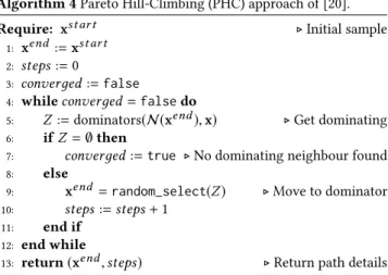
Algorithm 4Pareto Hill-Climbing (PHC) approach of [20].
Require: xst ar t ▷Initial sample
1: xend :=xst ar t 2: steps:=0
3: converдed:=false
4: whileconverдed=falsedo
5: Z:=dominators(N (xend),x) ▷Get dominating 6: ifZ=∅then
7: converдed:=true ▷No dominating neighbour found 8: else
9: xend =random_select(Z) ▷Move to dominator 10: steps:=steps+1
11: end if 12: end while
13: return(xend,steps) ▷Return path details
As outlined above, generating meaningful LONs using PLO is non-trivial. The set returned by PLS can intersect with that returned from a PLS started from a different solution, and therefore a solution may appear in multiple modes (in standard uni-objective LONs, a solution may contribute weight to multiple basins but a modal solution defines only one mode).
3.2
Dominance neutral optima
An alternative approach to define the landscape is to employ a point-basedlocal hill-climb to define a dominance-neutral neighbourhood [4]. Previous work to take such an approach to multi-objective land-scape analysis is the Pareto Hill-Climbing (PHC) approach of [20], which randomly moves a design in the hill-climb to a dominating neighbouring solution until no dominating neighbour was found. This approach is detailed in Algorithm 4.
It was asserted in [20] that the solution returned by PHC would be a member of anXP LO. However, this is not guaranteed, and indeed we observe that regularly this is not the case whenxst ar t <
Ð
iXP LOi . Figure 6 illustrates a simple counter example to the asser-tion that PHC results in a member ofXP LO, using the same data as illustrated in Figure 1. Nevertheless, such a point-based rather than set-based hill-climb is attractive from a practical point of view, as it does not require exhaustive enumeration of aXP LOfor a hill-climb to complete, and is therefore practical in a landscape approximation context (via sampling).
Using PHC results in dominance-neutral neighbourhoods (XD N O) comprised of solutions where each member is mutually non-dominated with immediate neighbouring members of the set, which we call dominance neutral optima (DNO). However, it does not ensure the set as a whole is comprised of mutually non-dominating solu-tions. In theory, this may lead to the pathological situation where
XD N O =X(or a substantial portion of it). This may arise when there aremanyobjectives, where the dominance measure is known to be less discriminating [1]. To be clear, in terms of set relationships:
Ð iXG P Oi ⊆ Ð jXP LOj ⊆ Ð mXmD N O ⊆X. 9,9 9,9 9,9 8,8 7,7 9,9 8,7 7,7 7,6 5,7 8,8 9,8 8,8 6,7 6,3 8,8 8,7 7,7 4,5 5,4 4,4 7,7 7,7 3,6 7,2 9,9 9,9 9,9 8,8 7,7 9,9 8,7 7,7 7,6 5,7 8,8 9,8 8,8 6,7 6,3 8,8 8,7 7,7 4,5 5,4 4,4 7,7 7,7 3,6 7,2
Figure 6: Example where PHC does not return a member of anXP LO. Left panel showsxst ar t in green, andxend in red
with the path in black (note how none of the neighbours ofxend dominate it). The right panel shows all dominance-neutral optima under PHC coloured red.Ð
jXD N Oj is a
su-perset ofÐ
iXP LOi .
Figure 7: PLOS-nets corresponding to the problems illus-trated in Figure 1 (left) and Figure 3 (right).
4
MULTI-OBJECTIVE OPTIMISATION
LANDSCAPES
We now describe existing work on representing multi-objective optimisation landscapes as graph, before presenting two new ap-proaches which embody many of the properties of LONs.
4.1
PLOS-nets
As mentioned in Section 1, PLOS-nets have recently been proposed as the first attempt to formulate a LON-like graph visualisation for multi-objective problems [10]. Although the term ‘Pareto local optima’ is used to describe the solutions defining the vertices in [10], they are actually defined in the work in terms of immediate neighbourhood non-dominance, and thus are not PLO (as defined in [15]). To avoid confusion, we will refer to the vertex solution properties in PLOS-nets as dominance neutral optima rather than Pareto local optima.
In PLOS-net construction, after the DNO are identified via enu-meration of the domain, the graph vertices are used to represent each DNO solution. Edges between vertices are formed if one solu-tion is a mutually non-dominating neighbour of another, resulting in an undirected graph. Figure 7 shows the PLOS-net graphs for the problems illustrated in Figure 1 and Figure 3. In keeping with [10], vertices are coloured according to their corresponding solution quality under theKth objective.
Algorithm 5PLON generation.
1: XP LO=∅ ▷Initial set of vertex sets
2: B=∅ ▷Initial map to basin size
3: C=∅ ▷Initial map to vertex colours 4: Esubset =∅ ▷Initial map of vertices to subsets 5: for∀x∈X do
6: P:=PLS(x) ▷Get resulting PLO set, see Algorithm 3 7: ifP,Xi
P LO∀XP LOi ∈XP LOthen ▷If newXiP LO 8: XP LO:=append(XP LO,P) ▷Add to list ofXi
P LO
9: BP :=1 ▷Initialise basin count
10: else
11: BP :=BP+1 ▷Increment basin count through map 12: end if 13: end for 14: for∀Xi P LO ∈XP LOdo 15: C Xi P LO :=count_GPO(Xi
P LO,XP LO)▷Get number of GPO 16: for∀Xj P LO∈XP LOdo 17: ifXj P LO⊂XiP LOthen 18: Esubset Xi P LO :=append(Esubset Xi P LO ,Xj P LO)▷Get covering 19: end if 20: end for 21: end for
22: E=get_edge_weights(XP LO,N ) ▷Generate edges 23: return(XP LO,B,C,E,Esubset)
4.2
Pareto local optima networks
Our first approach to transfer the LON to multi/many-objective problems is to initially identify the uniqueXi
P LOreturned by PLS, which may include intersectingXi
P LO. We can then identify all solutions which lead to each of theseXi
P LO, and therefore identify the basin sizes. There remains the issue that someXi
P LOmay be proper subsets of others, and therefore effectively their basin is larger than merely those members whose PLS lead to them exactly. We address this here by additionally highlighting directed edges where a mode completely contains the solutions defining another. We now describe the construction of LONs using PLS and PHC, which we call Pareto LONs (or PLONS). In PLONs the vertices represent theXi
P LOreturned from PLS. Their other properties are as follows:
(1) vertices are coloured proportional to the number of GPO they contain;
(2) the vertex radii are proportional to basin size;
(3) there is a directed edge between vertexAand vertexBif it is possible to move fromAtoBusing a transition to the other (illustrated using escape edges [18] here), with the width of the edge denoting the number of neighbours of the source
Xi
P LOwhich lead to this transition;
(4) highlighted edges denote if the destination is a subset of the source.
An algorithm outlining the generation of a PLON is provided in Algorithm 5. Example PLONs are provided in Figure 8 for the problems illustrated in Figure 1 and Figure 3.
Figure 8: PLONs corresponding to the problems illustrated in Figure 1 (left) and Figure 3 (right). Edges in red denote where theXP LO of the destination node is a subset of the
XP LOof the source node.
Algorithm 6DNON generation.
1: D=∅ ▷Initial set of dominance neutral locations 2: XD N O =∅ ▷Initial set of vertex sets
3: B=∅ ▷Initial map to basin size
4: C=∅ ▷Initial map to vertex colours 5: Esubset =∅ ▷Initial map of vertices to subsets 6: for∀x∈X do
7: Y :=PHC(x) ▷Get list of all locations resulting from PHC 8: for eachy∈Ydo 9: ify∈Dthen 10: By:=By+1 11: else 12: D=D∪ {y} 13: By:=1 14: end if 15: end for 16: end for
17: (XD N O,B):=agglomerate(D,B)▷Get walkable components 18: C:=get_number_of_GPO_per_vertex(XD N O)
19: E=get_edge_weights(XD N O,N ) ▷Generate edges 20: return(XD N O,B,C,E)
4.3
Dominance-neutral optima networks
Using PHC, andXD N O, we may construct Dominance-Neutral Optima Networks (DNONs) with the following properties:
(1) vertices are coloured by the number of GPO contained within the correspondingXi
D N O;
(2) the vertices represent the unique disjoint subsets of the
Xi
D N O, constructed by walking across solutions returned by PHC;
(3) the vertex radii are proportional to basin size (the proportion of walks from each solution inX where PHC leads to a member of theXi
D N O represented by the vertex);
(4) there is an edge between two verticesAandBif it is possible to move from one vertex to the other, with the width of the edge denoting how easy this is.
An algorithm outlining the generation of a DNON is provided in Algorithm 6. Example DNONs are provided in Figure 9 for the problems illustrated in Figure 1 and Figure 3.
Figure 9: DNONs corresponding to the problems illustrated in Figure 1 (left) and Figure 3 (right).
f1 f2 f3
f4 f5 Optima
Figure 10: Fitness landscapes under the five different rela-tively smooth objective functions. Bottom right panel high-lights the GPO, PLO and DNO sets.
f1 f2 f3
f4 f5 Optima
Figure 11: Fitness landscapes under the five different rela-tively rugged objective functions. Bottom right panel high-lights the GPO, PLO and DNO sets.
5
MANY-OBJECTIVE ILLUSTRATION
Our previous illustrations have been on small (|X|=25) bi-objective problems. We now illustrate the PLOS-net, PLON, and DNON on two larger (|X|=1600) five-objective (i.e. many-objective) prob-lems, one comprised of relatively smooth functions, and the other composed of relatively rugged functions. To aid visualisation and
Figure 12: PLOS-net (top-left), DNON (top-right) and PLON (bottom) for the problem illustrated in Figure 10.
Figure 13: PLOS-net (top-left), DNON (top-right) and PLON (bottom) for the problem illustrated in Figure 11.
understanding, we again use a problem where the search domain is in the plane. The images of these domains under the five different objective functions of the two problems are shown in Figures 10 and 11. The bottom right panel of each of these figures colours each cell (solution) by type. White are GPO, light grey are PLO (as are all black cells) and dark grey are DNO (as are all light grey and white cells). None of the black cells act as attractors under any optima category.
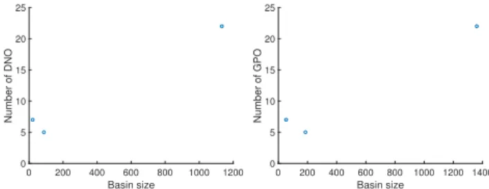
0 200 400 600 800 1000 1200 Basin size 0 5 10 15 20 25 Number of DNO 0 200 400 600 800 1000 1200 1400 Basin size 0 5 10 15 20 25 Number of GPO
Figure 14: DNON basin size versus number of DNO (left) and DNON basin size versus number of GPO (right) using the problem illustrated in Figure 11.
0 50 100 150 Basin size 0 20 40 60 80 Number of PLO 0 50 100 150 Basin size 0 5 10 15 20 Number of GPO
Figure 15: PLON basin size versus number of PLO (left) and PLON basin size versus number of GPO (right) using the problem illustrated in Figure 11.
In the smooth landscape with only a few minima under each indi-vidual objective, there are twoXi
P LOin the PLON, one of which is a subset of the other, and threeXj
D N O in the DNON, with the global Pareto optima split amongst two of them (see Figure 12). There is a marked contrast in the LONs generated for the rugged landscape. Again there are only threeXj
D N O using the DNON, although the basin sizes are different than for the first problem (the PLOS-net has correspondingly three maximal subgraph components). In con-trast, there are 93Xi
P LOunder the PLON representation — although nearly three-quarters of these are subsets of others (see Figure 13). The GPO are distributed amongst all vertices in both the DNON and PLON for this problem.
Figure 14 shows the distribution of basin size versus number of DNO in a vertex, and basin size versus the number of GPO in a vertex for the DNON on the rugged problem (correspondingly the number of vertices in each component of the PLOS-net). As can be seen, the distributions between the two subplots are fairly consistent, and the positive trend obvious (albeit on a small number of points). Figure 15 shows the distribution of basin size versus number of PLO in a vertex, and basin size versus the number of GPO in a vertex for the PLON on the rugged problem. In this particular instance there is a poor correlation between basin size and number of PLO or number of GPO (with a Spearman’sρof−0.31 and−0.17 respectively) — however, once basins which lead to vertices which are supersets of other vertices are taken into consideration we find the scatter plots in Figure 16, with a Spearman’sρ of−0.65 and−0.25 for the correlation between the augmented basin size
0 100 200 300 400
Augmented basin size
0 20 40 60 80 Number of PLO 0 100 200 300 400
Augmented basin size
0 5 10 15 20 Number of GPO
Figure 16: Augmented PLON basin size versus number of PLO (left) and augmented PLON basin size versus number of GPO (right) using the problem illustrated in Figure 11.
and PLO and GPO respectively, highlighting the difficulty of this particular problem.
As mentioned in Section 4.3, it is well-known that dominance becomes much less discriminatory as the number of objectives increases, making the landscape look largely neutral under local dominance comparisons. This is likely the root cause of the small number of vertices in the DNON representation, and PLOS-net com-ponents, though we have yet to undertake a rigourous examination of DNON properties as the number of objectives increases.
6
DISCUSSION
We have presented two new approaches for visualising multi/many-objective landscapes using the LON framework.
The first, the PLON exploits Pareto local search to build the LON and define the set memberships of each mode, mimicking the set-basednature of typical multi-objective search. Its construction is however relatively costly, and the inherent nature of theXi
P LO means there are two different forms of edges between vertices which require representation in the single graph. We note that alternatives could be to employ a graphpair representation, or employing a partitioned graph visualisation, akin to that used in e.g. [16] for funnels to denote this.
The second, the DNON uses point-based local search, with so-lutions requiring agglomeration after the individual Pareto hill-climbs have all completed to obtain the vertices. Nevertheless, its computational cost is much lower than the PLON, and the sets of so-lutions determining the vertices do not intersect. As such, it is more amenable to use in a estimation (sampling-based) context. It may also be effectively paired with the PLOS-net visualisation, to gain additional information as to how the separate DNO components are formed.
Although our illustrations are on problems with neighbourhoods on a grid, this was merely to aid visualisation and explanation. Both PLONs and DNONs may be applied generally to any multi-objective problem where a neighbourhood function is available for solutions, and we look forward to developing generic and efficient genera-tors for this (building on our previous work developing efficient packages in the uni-objective domain [3]).
Matlab code to regenerate the examples and visualisations in this paper is available at https://github.com/fieldsend.
ACKNOWLEDGMENTS
This work was supported by the Engineering and Physical Sciences Research Council [grant number EP/N017846/1].
REFERENCES
[1] David W. Corne and Joshua D. Knowles. 2007. Techniques for Highly Multiob-jective Optimisation: Some Nondominated Points Are Better Than Others. In Proceedings of the 9th Annual Conference on Genetic and Evolutionary Computation (GECCO ’07). ACM, New York, NY, USA, 773–780.
[2] Fabio Daolio, Sébastien Verel, Gabriela Ochoa, and Marco Tomassini. 2010. Local Optima Networks of the Quadratic Assignment Problem. InIEEE Congress on Evolutionary Computation. 1–8.
[3] Jonathan E. Fieldsend. 2018. Computationally Efficient Local Optima Network Construction. InProceedings of the Genetic and Evolutionary Computation Confer-ence Companion (GECCO ’18). ACM, New York, NY, USA, 1481–1488. [4] Jonathan E. Fieldsend, Tinkle Chugh, Richard Allmendinger, and Kaisa Miettinen.
2019. A Feature Rich Distance-Based Many-Objective Visualisable Test Problem Generator. InGenetic and Evolutionary Computation Conference, GECCO2019, Proceedings. ACM. https://doi.org/10.1145/3321707.3321727
[5] Tobias Glasmachers. 2017. A Fast Incremental BSP Tree Archive for Non-dominated Points. InInternational Conference on Evolutionary Multi-Criterion Optimization. Springer, 252–266.
[6] Leticia Hernando, Fabio Daolio, Nadarajen Veerapen, and Gabriela Ochoa. 2017. Local Optima Networks of the Permutation Flowshop Scheduling Problem: Makespan vs. total flow time. In2017 IEEE Congress on Evolutionary Compu-tation (CEC). 1964–1971.
[7] David Iclanzan, Fabio Daolio, and Marco Tomassini. 2014.Data-driven Local Optima Network Characterization of QAPLIB Instances. InProceedings of the 2014 Annual Conference on Genetic and Evolutionary Computation (GECCO ’14). ACM, New York, NY, USA, 453–460.
[8] Andrzej Jaszkiewicz and Thibaut Lust. 2018. ND-Tree-Based Update: A Fast Algorithm for the Dynamic Nondominance Problem.IEEE Transactions on Evolu-tionary Computation22, 5 (2018), 778–791.
[9] Joshua Knowles and David Corne. 1999. The Pareto archived evolution strategy: A new baseline algorithm for Pareto multiobjective optimisation. InEvolutionary Computation, 1999. CEC 99. Proceedings of the 1999 Congress on, Vol. 1. IEEE, 98–105.
[10] Arnaud Liefooghe, Bilel Derbel, Sébastien Verel, Manuel López-Ibáñez, Hernán Aguirre, and Kiyoshi Tanaka. 2018. On Pareto Local Optimal Solutions Networks. InParallel Problem Solving from Nature – PPSN XV, Anne Auger, Carlos M. Fon-seca, Nuno Lourenço, Penousal Machado, Luís Paquete, and Darrell Whitley
(Eds.). Springer International Publishing, Cham, 232–244.
[11] Gabriela Ochoa and Sebastian Herrmann. 2018. Perturbation Strength and the Global Structure of QAP Fitness Landscapes. InParallel Problem Solving from Nature – PPSN XV, Anne Auger, Carlos M. Fonseca, Nuno Lourenço, Penousal Machado, Luís Paquete, and Darrell Whitley (Eds.). Springer International Pub-lishing, Cham, 245–256.
[12] Gabriela Ochoa, Marco Tomassini, Sebástien Vérel, and Christian Darabos. 2008. A Study of NK Landscapes’ Basins and Local Optima Networks. InProceedings of the 10th Annual Conference on Genetic and Evolutionary Computation (GECCO ’08). ACM, New York, NY, USA, 555–562.
[13] Gabriela Ochoa, Nadarajen Veerapen, Darrell Whitley, and Edmund K. Burke. 2016. The Multi-Funnel Structure of TSP Fitness Landscapes: A Visual Exploration. InArtificial Evolution, Stéphane Bonnevay, Pierrick Legrand, Nicolas Monmarché, Evelyne Lutton, and Marc Schoenauer (Eds.). Springer International Publishing, Cham, 1–13.
[14] Gabriela Ochoa, Sébastien Verel, and Marco Tomassini. 2010. First-Improvement vs. Best-Improvement Local Optima Networks of NK Landscapes. InInternational Conference on Parallel Problem Solving from Nature. Springer, 104–113. [15] Luis Paquete, Tommaso Schiavinotto, and Thomas Stützle. 2007. On local optima
in multiobjective combinatorial optimization problems. Annals of Operations Research156, 1 (2007), 83.
[16] Sarah L Thomson, Fabio Daolio, and Gabriela Ochoa. 2017. Comparing commu-nities of optima with funnels in combinatorial fitness landscapes. InProceedings of the Genetic and Evolutionary Computation Conference. ACM, 377–384. [17] Marco Tomassini, Sébastien Vérel, and Gabriela Ochoa. 2008. Complex-network
analysis of combinatorial spaces: The NK landscape case.Physical Review E78 (Dec 2008), 066114. Issue 6.
[18] Sébastien Vérel, Fabio Daolio, Gabriela Ochoa, and Marco Tomassini. 2012. Lo-cal Optima Networks with Escape Edges. InArtificial Evolution, Jin-Kao Hao, Pierrick Legrand, Pierre Collet, Nicolas Monmarché, Evelyne Lutton, and Marc Schoenauer (Eds.). Springer Berlin Heidelberg, Berlin, Heidelberg, 49–60. [19] Sébastien Verel, Fabio Daolio, Gabriela Ochoa, and Marco Tomassini. 2018.
Sam-pling Local Optima Networks of Large Combinatorial Search Spaces: The QAP Case. InParallel Problem Solving from Nature – PPSN XV, Anne Auger, Carlos M. Fonseca, Nuno Lourenço, Penousal Machado, Luís Paquete, and Darrell Whitley (Eds.). Springer International Publishing, Cham, 257–268.
[20] Sébastien Verel, Arnaud Liefooghe, Laetitia Jourdan, and Clarisse Dhaenens. 2011. Pareto local optima of multiobjective NK-landscapes with correlated objectives. In European Conference on Evolutionary Computation in Combinatorial Optimization. Springer, 226–237.
[21] Sébastien Verel, Gabriela Ochoa, and Marco Tomassini. 2011. Local optima networks of NK landscapes with neutrality.IEEE Transactions on Evolutionary Computation15, 6 (2011), 783–797.