Conditional Volatility Nexus between Stock Markets and Macroeconomic Variables: Empirical Evidence of G-7 Countries

Journal of Economic Studies

Conditional volatility nexus between stock markets and macroeconomic variables: Empirical evidence of G-7

countries

Journal: Journal of Economic Studies

Manuscript ID JES-03-2017-0062.R2 Manuscript Type: Research Paper

Keywords: G-7 countries, stock market volatility, macroeconomic fundamentals, VAR models

Journal of Economic Studies

Conditional volatility nexus between stock markets and macroeconomic

3 4 5 6 7 8 9 10 11 12 13 14 15 16 17 18 19 20 21 22 23 24 25 26 27 28 29 30 31 32 33 34 35 36 37 38 39 40 41 42 43 44 45 46 47 48 49 50 51 52 53 54 55 56 57 58 59

variables: Empirical evidence of G-7 countries

David McMillan, University of Stirling

Shouyang Wang, University of the Chinese Academy of Sciences

Abstract

Purpose: The relation between stock market volatility and macroeconomic fundamentals for G-7 countries is analyzed using monthly data over the period from July 1985 to June 2015.

Methodology: The empirical methodology is based on two steps: in the first step, we obtain the conditional volatilities of stock market returns and macroeconomic variables through the GARCH family of models. We also incorporate the impact of early 2000s dotcom and the global financial crises. In the second step, we estimate multivariate vector autoregressive (VAR) model to analyze the dynamic relation between stock markets return and macroeconomic variables. Findings: The overall results for G-7 countries indicate a weak volatility transmission from macroeconomic factors to stock market volatility at individual level but the collective impact of volatility transmission is highly significant. Although, the results of block exogeneity indicate a bidirectional causality except for the UK, but the causal linkage is quite weak from stock market to macroeconomic variables. Moreover, the local financial variables excluding interest rate are closely integrated, and the volatility of industrial production growth and oil price are identified as the most significant macroeconomic factors that could possibly influence the directions of stock markets.

Originality: This research establishes the nature of the links between stock market and macroeconomic volatility. Research to date has been unable to satisfactorily establish the empirical nature of such links. We believe this paper begins to do this.

Journal of Economic Studies

1. Introduction.

Over the past few decades, as international stock markets have surged significantly, the issue of stock market volatility has become more prominent, especially during high volatility periods. The analysis of financial market volatility is crucial for asset pricing, risk management and fund allocation (Martens and Zein, 2004). Officer (1973) mentions that US stock market volatility was unusually high from 1929 to 1939 when compared to periods before and after. This view is supported by Schwert (1989), who reports that stock market volatility was high during major episodes in US economic history such as WWI, the great depression of 1929, WWII, the OPEC oil shocks and similar events. Karunanayake, et al. (2010) and Manda (2010) also report similar results regarding stock market volatility during the global financial crisis of 2008. Apart from such major events that significantly affect stock market volatility, noise trading and investor overreaction to macroeconomic news can also impact such volatility (Liljeblom and Stenius, 1997; French and Roll, 1986). Thus, understanding the relations between stock market and macroeconomic volatility is of importance to investors and other stakeholders, including policy makers, in order to know which factors affect stock market volatility and of any subsequent impact on the economy (Corradi et al., 2013). This issue forms the focus of the paper.

In relation to macroeconomic fundamentals, the initial work of, for example, Fama (1981), Schwert (1981), Geske and Roll (1983) and Pearce and Roley (1983) provides the theoretical underpinnings for the dynamic linkage between macroeconomic variables and stock market returns. Since then, an extensive discussion in the finance and economics literature on the sensitivity of stock markets to the macroeconomic uncertainty in both developed and emerging economies has occurred. The state of the literature is summed up aptly by Chen et al. (1986) who notes that we are yet unable to determine which economic variables are responsible for the

3 4 5 6 7 8 9 10 11 12 13 14 15 16 17 18 19 20 21 22 23 24 25 26 27 28 29 30 31 32 33 34 35 36 37 38 39 40 41 42 43 44 45 46 47 48 49 50 51 52 53 54 55 56 57 58 59

Journal of Economic Studies

movement of stock returns. In contrast, however, Chan et al. (1998) dismiss the empirical relevance of macroeconomic fundamentals on security returns. They argue that such exogenous factors make a poor showing in asset pricing and are as useful as any randomly generated series.

Although, the connection between systematic risk factors and the volatility of stock returns is intuitively appealing and can be theoretically motivated (Boudoukh and Richardson, 1993), there exists a large gap between the theoretical and empirical identification of such macroeconomic factors. The current study tries to bridge this gap by analyzing the volatility connectedness between stock returns and macroeconomic variables.

A sizeable empirical work has been advanced to study the linkage between the volatility of stock returns and macroeconomic fundamentals. For example, Schwert (1989) examines the relation of stock market volatility with the volatility of real and nominal macroeconomic series, financial leverage and trading volume by using monthly data from 1857-1987 for the US.1 He argues that although the volatilities of interest rate and corporate bond returns are correlated with the volatility of stock market returns, none of these play a dominant role in explaining the behavior of stock market volatility. Further studies examine the behavior of stock returns and inflation and the money supply (e.g., Fama, 1981; Geske and Roll, 1983; Pearce and Roley, 1983 find a negative relation). Erdem, et al. (2005) find a negative volatility spillover impact of inflation and a positive spillover impact of interest rate, exchange rate, money supply and industrial production on stock prices.

Like Schwert (1989), Morelli (2002) finds only a weak connection between stock market volatility and macroeconomic risk factors, notably industrial production index and money supply. Whereas, Diebold and Yilmaz (2007) report a positive linkage between macroeconomic

1

The initial work of Officer (1973), Black (1976), Shiller (1981), Fama (1981), Schwert (1981) Chen et al. (1986), Abel (1988), Campbell and Shiller (1988), French and Roll (1986) and Schwert (1989) laid the foundation for the work examining the nexus between stock market returns and macroeconomic uncertainty.

3 4 5 6 7 8 9 10 11 12 13 14 15 16 17 18 19 20 21 22 23 24 25 26 27 28 29 30 31 32 33 34 35 36 37 38 39 40 41 42 43 44 45 46 47 48 49 50 51 52 53 54 55 56 57 58 59

Journal of Economic Studies

volatility and stock market volatility in a global perspective. Similarly, Chinzara (2011) finds a positive volatility spillover from the T-bill rate, exchange rate and gold price while negative volatility spillovers arise from inflation. Narayan and Gupta (2015) find that the oil price is a significant predictor of stock returns. By using monthly data over the period of one and half century long for US, they find that negative oil price shocks are more significant in predicting stock returns as compared to positive shocks. Diaz et al., (2016) also document a negative response of stock market volatility to oil price volatility.

The main motivation of our research is to examine how macroeconomic volatility affects stock market volatility in G-7 countries. Our research will thus compliment and extend the existing literature (e.g., Wongbangpo and Sharma, 2002; Diebold and Yilmaz, 2007; Yartey, 2008; Diaz, et al., 2016), which will also provide a point of comparison, especially given the number of crises that have occurred over the last 30-years period.2 Of perhaps particular relevance is the impact of the two most recent crises that began with the bursting of the dotcom bubble as well as the global financial crisis. Moreover, while the work of Diebold and Yilmaz (2007) covers a wide range of markets, none of the previous research considers the impact of crisis periods on aggregate stock market returns in the framework of macroeconomic fundamentals.

The present study contributes in several ways; first, it uses an updated monthly data set covering the last 30-years for the G-7 countries, except France and Italy.3 The use of both monthly data and a long sample period should ensure robust results that would help financial

2

The most prominent crises that took place during our sample period are OPEC collapse in 1986, Black Monday on October 19, 1987, early 1990s recession, Japan stock market collapse in early 1992, Asian financial crises, Russian and Brazilian financial crises, Argentina economic depression, dotcom bubble crash, 9/11 terror attacks, global financial crises of 2008, Russian oil market crash and the euro debt crisis.

3

Data availability problem restricted us to use 30-years data for France and Italy. For France, we have used data for almost 25-years monthly data that starts from January 1990 to June 2015 while for Italy we have used 18.5-years monthly data that covers from December 1997 to June 2015.

3 4 5 6 7 8 9 10 11 12 13 14 15 16 17 18 19 20 21 22 23 24 25 26 27 28 29 30 31 32 33 34 35 36 37 38 39 40 41 42 43 44 45 46 47 48 49 50 51 52 53 54 55 56 57 58 59

Journal of Economic Studies

analysts and policy makers in improved decision-making. Second, we consider the effect of crisis periods through the inclusion of two dummy variables for the early 2000s crisis and global financial crisis of 2008 respectively. Third, we investigate the relation between the volatilities of stock market and macroeconomic variables (industrial production, money supply, interest rate, inflation, exchange rate and oil price) in a multiple country perspective, allowing us to make comparisons. Overall, we hope that the findings of this study will be of interest to investors, financial analysts and policy makers.

The remainder of this study is organized as follows. Section 2 presents the data and descriptive statistics and Section 3 explains the econometric methodology of this study. Section 4 and Section 5 present the empirical results and the concluding remarks respectively.

2.Data

2.1. Data and variables

The stock markets data used in this study are comprised of monthly indices of aggregate stock markets of G-7 countries.4 The data is obtained over the time-period from July 1985 to June 2015. The time series plots of the stock market indices are displayed in Figure 1 and indicates that stock market indices follow a random walk pattern. As can be observed, while there are numerous up and down movements there are two noticeable downward swings for all G-7 countries except Japan, which has experienced less stock market growth since the 1980s. These coincide with the early 2000s dotcom crash and the global financial crisis.

The macroeconomic variables to be used in study are industrial production index (IPI),

4

Dow Jones Industrial Average (DJIA) Index for USA, Financial Times Stock Exchange 100 Index for UK, Toronto Stock Exchange Index for Canada, Nikkei225 Index for Japan, German Deutscher Aktien Index(GDAXI) for Germany, CAC40 Index for France and FTSE MIB-30 Index for Italy. The data is obtained from DataStream.

3 4 5 6 7 8 9 10 11 12 13 14 15 16 17 18 19 20 21 22 23 24 25 26 27 28 29 30 31 32 33 34 35 36 37 38 39 40 41 42 43 44 45 46 47 48 49 50 51 52 53 54 55 56 57 58 59

Journal of Economic Studies

consumer price Index (CPI), broad money supply (M2), treasury bill rate (TBR),5 exchange rate with respect to the US dollar (ER)6 and crude oil price in local currency (OIL).7 This selection of the variables is based on the theoretical relevance of these variables to the stock market index as supported by the existing literature (Schwert, 1989, Morelli, 2002; Flannery and Protopapadakis, 2002; Gan, et al. 2006; Chinzara, 2011; Hsing and Hsieh, 2012; Su et al., 2014; Kumari and Mahakud, 2015). All the data series are converted into growth form by using first-difference logarithmic transformation (∆LnYt = LnYt – LnYt-1). Majority of macroeconomic data series and

stock market indices for G-7 countries are collected from the online Thomson Reuters DataStream and CEIC global data base.8 We also used Organization of Economic Co-operation and Development (OECD) data source to collect the missing data on short term interest rate for Japan, France and Italy.

2.2. Stability diagnostics for G-7 stock markets return

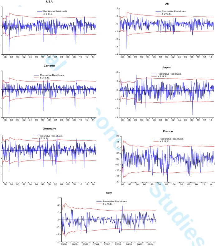
Our data for the G7 stock markets covers a history of three decades. Therefore, it is possible that the data contains structural breaks. For this purpose, we estimate the recursive residuals from an AR model (discussed below) with plus/minus two standard errors, which are displayed in Figure 2. Evident in the plots of the recursive residual are various low and high extremes. Of particular interest are those that cross the standard error bounds, which appear evident during the stock market crash in 1987, Asian financial crisis, early 2000s crisis and the global financial crisis.

5

Six months Treasury Bill rate has been used for USA, UK, Canada and Italy and Short term interest rate collected from OECD website (https://data.oecd.org/) for Japan, Germany and France.

6

Exchange rate for USA has been taken as units of USD per Euro 7

Oil Price is the WTI spot price in local currency, which is calculated using the exchange rate as per USD.

8

CEIC is a European institutional investor company founded in 1992 that provides most expansive and accurate economic and financial data about the emerging and developed markets. The CEIC global database was accessed from the School of Management, university of Chinese Academy of Sciences Beijing, China.

3 4 5 6 7 8 9 10 11 12 13 14 15 16 17 18 19 20 21 22 23 24 25 26 27 28 29 30 31 32 33 34 35 36 37 38 39 40 41 42 43 44 45 46 47 48 49 50 51 52 53 54 55 56 57 58 59

Journal of Economic Studies

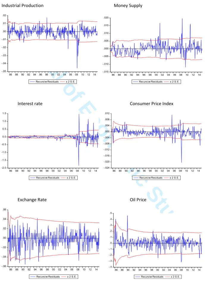
Therefore, the current study uses dummy variables to captures the impact of crises periods.9 For consistency, we also consider a similar exercise for the macroeconomic variables, to illustrate Figure 3 reports the plots for the US. As can be observed from this figure, we can see the potential for breaks occurring over the same time-period as those for the stock returns. Notably, this is for the financial crisis period and, to a lesser extent, the bursting of the dotcom bubble. Thus, the dummy variables we include, as noted above, appear to be appropriate for the macroeconomic series.10

2.3. Descriptive summary and unit root tests

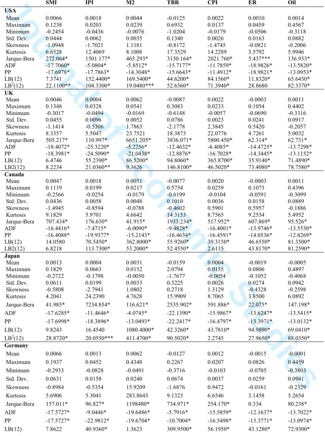
Descriptive statistics and unit root test results for the stock returns and macroeconomic growth rates are presented in Table 1. The results indicate that the average of stock market return is highest for US and Germany, followed by Canada, UK, France, Japan and Italy. The average stock market return for Italy not only stands lowest in the list of G-7 countries but is in fact negative, while Italy also has the highest standard deviation. The stock markets of the US, UK and Canada have a relatively lower standard deviation compared to the markets of Japan and Germany. Overall, we can nonetheless observe the usual characteristics whereby the financial data are more volatility than the macroeconomic data. For unit root testing, both the Augmented-Dickey Fuller (ADF) and Phillips-Perron (PP) tests show that all the growth series are stationary.11 Ljung-Box (LB) tests for return series and squared return series were also performed to check the serial correlation and ARCH effect, and the results of these tests justify the

9

The current study only uses two dummy variables that captures the impact of early 2000s crisis period and the global financial period of 2008 for all G-7 countries. Although, for Japan there appears to be no stability problem during the early 2000s, but for sake for uniformity of dummy selection, we include this dummy for Japan. The insignificance of the dummy variable for Japan during the early 2000s crisis period will also serve as a validity check for this dummy variable.

10

The plots for the remaining countries are available upon request. 11

For the sake of completeness, the levels of the series all contain a single unit root.

3 4 5 6 7 8 9 10 11 12 13 14 15 16 17 18 19 20 21 22 23 24 25 26 27 28 29 30 31 32 33 34 35 36 37 38 39 40 41 42 43 44 45 46 47 48 49 50 51 52 53 54 55 56 57 58 59

Journal of Economic Studies

application of GARCH models to capture the volatility of monthly data series for stock market returns and other macroeconomic variables.

3. Methodology

To analyze the dynamic relation between stock market volatility and macroeconomic risk factors we use a vector autoregressive (VAR) model. A significant body of the literature (Liljeblom and Stenius, 1997; Errunza and Hogan, 1998; Morelli, 2002; Chinzara, 2011; Kumari and Mahakud, 2015) has previously considered this approach. Prior to the application of the VAR model, we first capture the stock market and macroeconomic volatilities using a GARCH model.

3.1. GARCH model specifications

The autoregressive conditional heteroscedasticity (ARCH) model was introduced by Engle (1982) before Bollerslev (1986) extended the model to the generalized ARCH (GARCH) model. This model employs a maximum likelihood procedure and allows the conditional variance to be vary over time. This model is now widely used to capture the volatility clustering effect observed in many data series. In the application of the model here, we include two dummy variables to capture the effect of the crises noted above.12 The GARCH(p,q) model is specified as follows:

1 , k t i i t i t i r µ a r₋ ε = = +

∑

ε

Dum1is used to account for the early 2000s crises originating from the US dotcom bubble crash and the 9/11 terror attacks. The dummy covers the period from March 2000 to October 2002, and almost all G-7 countries were affected over this period. Dum2 is used to capture the global financial crisis (GFC) that cover the period from July 2007 to June 2009. In terms of other possible dummies, an obviously period would be 1987. However, we do not include a dummy here. This is because, although, there was a market crash on October 19, 1987 and the Dow Jones industrial average index plunged about 500 points, the market partially rebounded the next day. Moreover, there was no lasting economic effect, as economic growth continued to be positive. Hence, this period differs from the dotcom and financial crisis periods that had a longer lasting economic impact.

3 4 5 6 7 8 9 10 11 12 13 14 15 16 17 18 19 20 21 22 23 24 25 26 27 28 29 30 31 32 33 34 35 36 37 38 39 40 41 42 43 44 45 46 47 48 49 50 51 52 53 54 55 56 57 58 59

Journal of Economic Studies

ω

α ε

β

γ

γ

∑

∑

ω

α

β

returns. The current innovation term, εt is conditioned on a previous information set It-1 with zero

mean, a variance ht and is serially uncorrelated, rt and rt-i denote the current and lagged returns respectively. Equation (2) is a GARCH(p,q) variance equation, where ht is the conditional variance, ωi is constant, αi is the coefficient of the lagged squared residuals from the mean

equation and βj is the coefficient for the lagged conditional variance. Dum1=1 for the early 2000s

crises period, otherwise 0, Dum2=1 if for the GFC period, otherwise 0 and γ1 and γ2 are the

coefficients of dummy variables respectively.

One assumption underlying the standard GARCH model is the symmetry of shocks on volatility. However, it is argued that negative shocks should have a greater impact on volatility than positive shocks of an equal magnitude. Therefore, we consider the exponential-GARCH (EGARCH) model of Nelson (1991). The model is given by:

1 1 2 2 1 1 1 log( ) log q m p t i t i t k t i i k j t j i _{t i t i} k _{t k} j h E h Dum Dum h h h ε ε ε ω α − − γ − β ϕ ϕ − = _{− −} = ₋ =  _{ }   = + − _ _ + + + +  _{ }  

∑

∑

∑

Where γk is the coefficient of asymmetric component and if it is significant and negative then

negative (or bad news) brings higher volatility compared to positive news of the same magnitude. In the empirical application below we consider both the GARCH and EGARCH models and select the preferred model according to Akaike Information Criterion (AIC).

3.2. VAR Models

The specification of the VAR model to analyze the relation between the conditional volatility of stock markets and macroeconomic variables is as follows.

3 4 5 6 7 8 9 10 11 12 13 14 15 16 17 18 19 20 21 22 23 24 25 26 27 28 29 30 31 32 33 34 35 36 37 38 39 40 41 42 43 44 45 46 47 48 49 50 51 52 53 54 55 56 57 58 59

Journal of Economic Studies

ε

∑

Where, hit is the time varying column vector of stock market volatility and macroeconomic variables volatilities of G-7 countries. ci is a 7x1 deterministic component of a constant, m is the

lag length for 7x7 matrix coefficients and εit is 7x1 residual vector which is not correlated to the

past values of ht-s contemporaneously.

Although, the VAR model is a very useful technique to examine interrelations between variables, the interpretation of the results can become complicated when the coefficient sign on variable changes across lags. Thus, to determine the impact on future values on other variables in the VAR system we examine the impulse response functions (IRFs) and the forecast variance decompositions.

4. Empirical Results and Discussion 4.1. GARCH models results and discussion

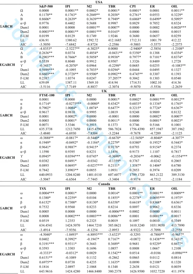
GARCH models are estimated for all stock markets return and macroeconomic variables for the G-7 countries with the results are presented in Table 2. The conditional mean model (not reported) was estimated according to an ARMA specification.13 The results of the volatility models with dummy variables show evidence volatility persistence in all the stock return and macroeconomic growth series except for exchange rate and oil prices for France and CPI and exchange rate for Italy. The results of EGARCH model show clear evidence of asymmetry in all the stock markets return except UK. In case of macroeconomic variables, the asymmetry coefficient (γ) of industrial production, short-term interest rate and oil price is significant for

13

In most of the series we only added a AR(1), MA(1) or ARMA(1,1) in the mean equation in order to ensure a white noise error term although in a few cases the AIC and SIC values were lowest at higher order ARMA process.

3 4 5 6 7 8 9 10 11 12 13 14 15 16 17 18 19 20 21 22 23 24 25 26 27 28 29 30 31 32 33 34 35 36 37 38 39 40 41 42 43 44 45 46 47 48 49 50 51 52 53 54 55 56 57 58 59

Journal of Economic Studies

most G-7 countries. Whereas, the asymmetry coefficient of money supply, inflation and exchange rate is insignificant for all countries except for CPI for UK that has significant γ. The results of EGARCH model show that the overall response the volatilities of stock market returns and macroeconomic variables to the market news is identical. The significant and negative value of asymmetry coefficient indicates that the negative news has a greater impact on the volatility of stock markets return and macroeconomic variables, than positive news of same magnitude. These results are consistent with findings within the literature (e.g., Schwert, 1989; Campbell and Hentschel, 1992; Koutmos and Booth, 1995; Chinzara, 2011, Kumari and Mahakud, 2015).

The dummy coefficients are significant in all the stock markets return except UK. For the macroeconomic variables, industrial production index has structural breaks for all countries. M2 TBR and CPI also have structural breaks for all countries except for M2 for the UK. Similarly, exchange rate has structural breaks for all countries except France and Germany. Finally, the results of oil price data do not indicate any structural break for USA, Canada, Japan, France and Germany. Most of the significant coefficients of dummy variables are negative which indicate that during the crisis period volatility is much higher as compared to non-crisis period.

3.2 VAR models results and discussion

Having obtained the conditional volatilities for the stock market and macroeconomic series from the appropriate GARCH model, we now estimate a system of simultaneous equations using the vector autoregressive (VAR) framework. The appropriate lag length is selected by AIC lag selection criteria.14 After selecting the lag length, we estimate block exogeneity (F-statistics) to analyze the causal connection between the volatilities of the macroeconomic variables on stock

14

In addition to the AIC we also consider the BIC and FPE (final prediction error). In each case the AIC and FPE choose the same lag length, as does the BIC for three markets. For the remaining markets the BIC chooses a shorter lag length. We opt for the AIC/FPE lag length to avoid the potential issue of selecting too short a lag length.

3 4 5 6 7 8 9 10 11 12 13 14 15 16 17 18 19 20 21 22 23 24 25 26 27 28 29 30 31 32 33 34 35 36 37 38 39 40 41 42 43 44 45 46 47 48 49 50 51 52 53 54 55 56 57 58 59

Journal of Economic Studies

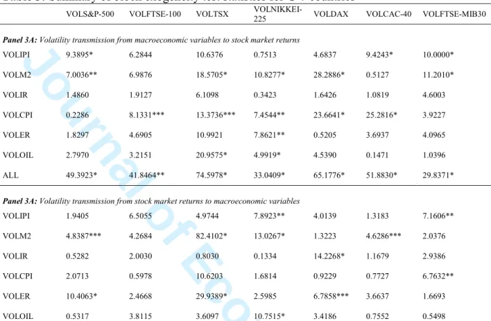
market returns. One important issue concerns the identification of the VAR in which the ordering of variables is important (Mills and Mills, 1991). To consider this, we estimate various combinations of the given variables in our VAR system, while the reported results are the ones that are robust with respect to different possible orderings of the variables. The results of the block exogeneity tests for volatility transmission between the macroeconomic and stock markets variables are presented in Table 3.

The results in Panel-3A of Table 3 show the volatility transmission from macroeconomic factors to stock market returns. These results indicate that the volatility of industrial production growth and money supply significantly influence US stock market volatility. For the UK, only CPI is found to significantly affect stock market volatility, while for Canada, Japan, Germany, France and Italy the volatility of the monetary variables (money supply and CPI) significantly impact stock market volatility. The volatility of industrial production growth is also a significant macroeconomic factor for stock market volatility for France and Italy. These results partly confirm those previously reported in the literature (e.g., Erdem, et al. 2005; Diebold and Yilmaz 2007 and Chinzara, 2011). Oil price volatility is also identified as an important determinant of stock market volatility in Canada and Japan. As oil is a major input for economic activity, it is plausible that oil price fluctuations would influence the level of output through production costs and the prices of consumer goods, which in turn will affect household consumption and profitability of firms. Of the markets considered here, Canada is the largest exporter of oil, while Japan is the second largest importer of oil, after the US, which is also an oil producer and thus, less impacted by oil price fluctuations. Diaz et al., (2016) also report a strong connection between oil price volatility and stock market returns in their study on G-7 countries.

In case of Japan, the volatility of money supply, inflation, exchange rate and oil price are

3 4 5 6 7 8 9 10 11 12 13 14 15 16 17 18 19 20 21 22 23 24 25 26 27 28 29 30 31 32 33 34 35 36 37 38 39 40 41 42 43 44 45 46 47 48 49 50 51 52 53 54 55 56 57 58 59

Journal of Economic Studies

significant factors affecting stock market volatility. Thus, we observe more interaction from the macroeconomic variables. This may be because the Japanese economy has faced a difficult situation for the past two decades, starting from the late 1980s and which has been accompanied by unorthodox monetary policy. A possible reason for the stronger integration between the volatility of the monetary and stock market variables could be accredited with the fact that the exchange rate (yen/dollar) was a dominant factor affecting monetary policy and trade tensions between the US and Japan, especially in the first decade of our sample period. Indeed, the exchange rate was subject to political influence, which affected market expectations (McKinnon and Ohno, 1997).

The above results provide evidence of significant macroeconomic volatility transmission to the volatility of stock market returns for all G-7 countries. The results of volatility transmission from stock market to macroeconomic variables are presented in Panel-3B of Table 3. The findings of the block exogeneity test indicate volatility transmission from stock market to macroeconomic variables for all G-7 countries except the UK. The results for UK indicate that there is a unidirectional volatility transmission moving from macroeconomic variables to stock market return, while for the rest of countries it is bidirectional. The results of causality linkage between the volatilities of stock markets return and macroeconomic variables for the UK are in line with Morelli (2002), who also reports a weak volatility connection between macroeconomic variables and stock market returns for the UK.

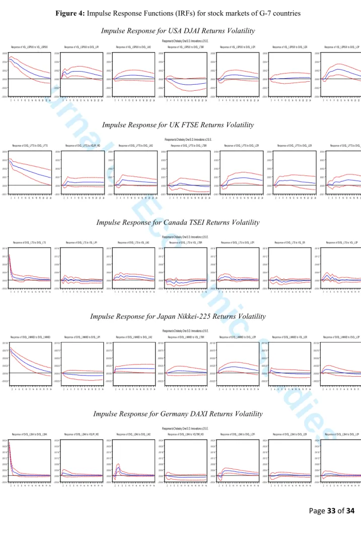
To analyze the speed, direction and persistence of stock market volatility in response to macroeconomic shocks, we estimate 24-month impulse response functions, which are reported in Figure 4. 15 Generally, the response of stock market volatility to the innovations of

15

Results of remaining IRFs of other macroeconomic variables were also estimates in the VAR system, but for space interest, all results are not reported here and can be made available on request.

3 4 5 6 7 8 9 10 11 12 13 14 15 16 17 18 19 20 21 22 23 24 25 26 27 28 29 30 31 32 33 34 35 36 37 38 39 40 41 42 43 44 45 46 47 48 49 50 51 52 53 54 55 56 57 58 59

Journal of Economic Studies

macroeconomic variables is quite persistent. There is a positive response of stock market volatility to the one standard deviation innovation of industrial production volatility (VOLIPI) over the 24-months horizon period for all G-7 countries except Canada and Japan. In case of Canada, the response is initially positive and then after one year it becomes negative while for Japan it is insignificant and negative. We note that for the US and Italy, the positive impact of VOLIPI on stock market volatility becomes significant and sustainable after the 12th and 20th month respectively, while for UK, Germany and France it remains insignificant over the 24-months horizon period. The results are similar to Schwert (1989) and Morelli (2002).

The response of stock market volatility to money supply volatility (VOLM2) shocks is positive for all countries except France where it is initially positive but over the long run it becomes negative. The literature has also reported mix results about the response of stock market to money supply.16 The results for France are in the line with (Grossman, 1981; Urich and Wachtel, 1981; Pearce and Roley, 1983; Gan, et al. 2006 and Adjasi, 2009). The negative response of stock market volatility to money supply growth volatility can be rationalized through the behavior of investors who assume that the central bank will tighten monetary policy when inflationary expectations rise. This anticipation of restrictive monetary policy would trigger investors to sell their securities leading to a higher expected future rate of return.17 That said, investors may have different expectations about the inflation when stock markets respond positively to the monetary shocks (Fama and Schwert, 1977 and Fama, 1981). A counter

16

Mukherjee and Naka (1995) argue that analyzing the impact of money supply shocks to stock markets is an empirical question and that results can vary depending upon the selections of sample data sets, countries, measures of variables used. So, the results can be different for different researchers and this argument was found to be true after examining the results of mentioned studies in the literature, some researchers have found positive relation while others have found negative between money supply and stock prices volatility.

17

See Gan, Lee, Yong, and Zhang (2006) found a negative response of New Zealand stock market volatility to money supply (M1) shocks. Similarly, the consensus finding from the studies of Grossman, 1981; Urich and Wachtel, 1981; Pearce and Roley, 1983) is that they all have associated the higher interest rate to the high unexpected money growth and that would lead to lower the stock prices.

3 4 5 6 7 8 9 10 11 12 13 14 15 16 17 18 19 20 21 22 23 24 25 26 27 28 29 30 31 32 33 34 35 36 37 38 39 40 41 42 43 44 45 46 47 48 49 50 51 52 53 54 55 56 57 58 59

Journal of Economic Studies

argument in favor of a positive response of stock market volatility to money supply has also been made (e.g., Friedman and Schwartz, 2008; Muradoglu and Metin, 1996; Bailey, 1988; Maysami and Koh, 2000). This line of research argues that money growth would lead to an increase in liquidity and the purchasing power of consumers that would ultimately lead to an increase in the price of stocks.

The results of impulse response functions of stock market volatility with respect to one standard deviation innovations in the Treasury bill (VOLTBR) indicate a negative response for all stock markets except the Nikkei 225 for Japan. This negative response is consistent with Chinzara (2011), who reports similar results for South Africa. The positive response of Japanese stock market volatility to VOLTBR is in line with the findings of Kumari and Mahakud (2015) for India. That said, the stock market volatility response in this case is only significant for the US and Canada in short-run otherwise. The response of stock market volatility to inflation shocks is positive and mainly significant over the short and medium term for all countries except the US and Italy. Once again, the challenge of mixed results is persistent because Adjasi, (2009) among others finds a negative response of stock market volatility to inflation rate while positive response to the interest rate shocks.

A mixed response of stock market volatility to exchange rate volatility (VOLER) is also observed. For the US and UK, it appears positive over the horizon period while for rest of the countries the spontaneous response of stock market volatility is negative but over the long run it also becomes positive. However, the response of the Japanese market is opposite to the other stock markets. In short run, the response of the Japanese market is positive, but over the long run it becomes negative. A possible reason for this behavior can be given by McKinnon and Ohno (1997), who argue that the underlying factors of exchange rate (yen/dollar) movements certainly

3 4 5 6 7 8 9 10 11 12 13 14 15 16 17 18 19 20 21 22 23 24 25 26 27 28 29 30 31 32 33 34 35 36 37 38 39 40 41 42 43 44 45 46 47 48 49 50 51 52 53 54 55 56 57 58 59

Journal of Economic Studies

affect market behavior, while policy failed to provide direction for the exchange rate. Wangbangpo and Sharma (2002) also find a mixed relation between stock prices and exchange rate for some emerging Asian economies (Malaysia, Indonesia, Singapore, Thailand and Philippine). Surprisingly, the response of stock market volatility to oil price volatility (VOLOIL) is insignificant and positive for the US, UK and Germany. These results are contradictory to Diaz et al., (2016), who find a negative response of G-7 stock markets to an increase in oil prices. For Canada, Japan, France and Italy, the response of stock market volatility is negative to VOLOIL, but it significant only for Canada and Japan. The overall results of impulse response functions are in line with the block exogeneity results in Table 3. Moreover, it can be observed from the impulse response functions that the relation between stock market volatility and macroeconomic factors is indeed bidirectional.18 Thus, there is also evidence of significant volatility response of macroeconomic variables to the volatility of stock markets returns for all G-7 countries.

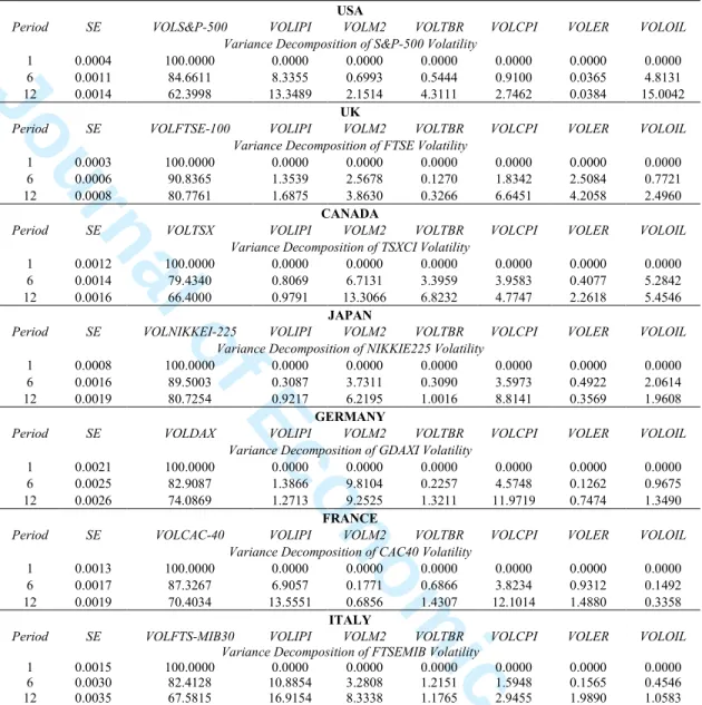
In order to provide further analysis of our results, we now consider the variance decompositions, which reveal proportion of stock market volatility that is explained by the macroeconomic volatility and vice versa. For this purpose, we estimate 12-period forecast for the variance decomposition with the results presented in Table 4.19

Examining these results, it can be observed that the movement of volatility of stock market returns, for most the G-7 countries, arises from their own shocks. However, it is noticeable that some macroeconomic variables contribute to stock return volatility. At the 12th period lag, about 38% of the variation in US stock market volatility is explained by the volatility

18

The results of IRFs are only reported here partially; the complete results are available with the authors and can be made available to the reviewers on demand.

19

The results of 12 periods forecast variance decomposition are only reported here for stock markets of G-7 countries. The complete results are not reported here due to space reasons and can be made available upon request.

3 4 5 6 7 8 9 10 11 12 13 14 15 16 17 18 19 20 21 22 23 24 25 26 27 28 29 30 31 32 33 34 35 36 37 38 39 40 41 42 43 44 45 46 47 48 49 50 51 52 53 54 55 56 57 58 59

Journal of Economic Studies

of other macroeconomic variables. For the other markets, the equivalent figures are about 20% of the variation in UK and Japanese stock return volatility, 34% of the variations in the Canadian and Italian stock market and 26% and 30% for German and French markets respectively.

Examining these results in greater detail, for the US the main contributing factors are oil (VOLOIL) and industrial production (VOLIPI), contributing 15% and 13.35% respectively. For the UK, the highest contribution is made by consumer prices (VOLCPI), however, this is only 6.64%, with more than 80% of the variation arising from the stock market itself. For Canada oil and money supply (VOLM2) are the main factors, explaining 5.45% and 13.31% of the variation in stock market volatility. In case of Japan and Germany, money supply and consumer prices are the highest contributing factors, while for France, consumer prices and industrial production are the main contributing series. Finally, for Italy VOLIPI and VOLM2 contribute 17% and 8% respectively to stock market volatility.

In terms of the reverse effect, the 12-period forecast variance decomposition reveal a weak contribution from stock market volatility to macroeconomic volatility. For Canada, stock market volatility contributes 8.6% of the movement in money supply growth volatility. For Japan, we observe 12% and 6% from stock market volatility to VOLIPI and VOLOIL respectively, while only 6% of the variation in VOLTBR arises form stock market volatility for Germany. Overall, these results reveal a weak contribution of macroeconomic volatility to stock market volatility and vice versa for our markets. This weak connection has previously been observed by Schwert (1989). Whereas, Chinzara (2011) and Kumari and Mahakud (2015) reported a strong feedback connection from stock market volatility to macroeconomic uncertainty for emerging markets (i.e. South Africa and India).

To summarize, the empirical linkage between stock market volatility and the systematic

3 4 5 6 7 8 9 10 11 12 13 14 15 16 17 18 19 20 21 22 23 24 25 26 27 28 29 30 31 32 33 34 35 36 37 38 39 40 41 42 43 44 45 46 47 48 49 50 51 52 53 54 55 56 57 58 59

Journal of Economic Studies

risk factors remains unclear. Although the collective impact of systematic risk factors to stock market volatility is significant as shown by block exogeneity results, it is weak at the individual macro-series level. Of note, it would appear unexpected to find no significant relation arising from short-term interest rates. Generally, short-term interest rates are considered as perhaps the most important factor in stock market volatility as interest rate play a crucial role in determining both macroeconomic health and firm level decisions around the appropriate capital structure and investment plans. That said, the volatility of money supply growth is identified as the most dominant factor of macroeconomic volatility. Further, the significant dummy coefficients in EGARCH model for stock market returns and most of the macroeconomic variables indicate the potential for structural breaks. It may be that issues surrounding stability within the data can have a strong influence on the potential stock market and macroeconomic volatility nexus.

5. Concluding Remarks.

This paper considers the relation between stock market and macroeconomic volatility for the G-7 markets using monthly data over the period July 1985 to June 2015. In conducting the analysis, we take explicit account of two major crisis periods (the dotcom crash and the global financial crisis). We obtain the conditional volatilities of both stock market and macroeconomic variables by estimating GARCH-type models. The volatilities are then used in a VAR model in order to consider the linkages. The GARCH models reveal the usual characteristics of volatility persistence, with asymmetric behavior in the stock market returns as well as some of the macroeconomic variables (industrial production, short-term interest rate and oil price). Furthermore, the GARCH results reveal a significant impact of the crisis periods on the majority of the volatility series.

3 4 5 6 7 8 9 10 11 12 13 14 15 16 17 18 19 20 21 22 23 24 25 26 27 28 29 30 31 32 33 34 35 36 37 38 39 40 41 42 43 44 45 46 47 48 49 50 51 52 53 54 55 56 57 58 59

Journal of Economic Studies

The VAR results reveal that the volatility transmission impact of industrial production, money supply and inflation is positive, for interest rates it is insignificant and negative for all countries except Japan, while for the exchange rate and oil prices the spillover impact is mixed across the different markets. The relation between stock market volatility and macroeconomic volatility unidirectional for UK, while for the rest of G-7 countries, causality is bidirectional, although it may not always be strong. Of particular note, money supply and exchange rate volatility has strong bidirectional causality with stock market volatility for the majority of countries.

Overall, the bidirectional causality highlights the nature of interdependence of macroeconomic fundamentals and stock market returns. This, in turn, is important for policy makers, investors and risk managers who should incorporate these interrelations into their decision making. As a final point, we have included dummy variables to account for the dotcom and financial crisis periods. Our results show that accounting for these periods is important. An extension to this work could be to consider further periods of market stress at both the local and regional as well as global level. This should further improve our understanding of the nature of the linkages between the stock market and the macroeconomy.

3 4 5 6 7 8 9 10 11 12 13 14 15 16 17 18 19 20 21 22 23 24 25 26 27 28 29 30 31 32 33 34 35 36 37 38 39 40 41 42 43 44 45 46 47 48 49 50 51 52 53 54 55 56 57 58 59

Journal of Economic Studies

References

Abbas, G., & McMillan, D. G. (2014). Interaction among stock prices and monetary variables in Pakistan. International Journal of Monetary Economics and Finance, 7(1), 13-27.

Abel, A. B. (1988). Stock prices under time-varying dividend risk: An exact solution in an infinite-horizon general equilibrium model. Journal of Monetary Economics, 22(3), 375-393.

Adjasi, C. K. (2009). Macroeconomic uncertainty and conditional stock-price volatility in frontier African markets: Evidence from Ghana. The Journal of Risk Finance, 10(4), 333-349.

Bailey, W. (1988). Money supply announcements and the ex ante volatility of asset prices.

Journal of Money, Credit and Banking, 20(4), 611-620.

Bollerslev, T. (1986). Generalized autoregressive conditional heteroskedasticity. Journal of Econometrics, 31(3), 307-327.

Boudoukh, J., & Richardson, M. (1993). Stock returns and inflation: A long-horizon perspective.

The American Economic Review, 83(5), 1346-1355.

Brooks, C. (2014). Introductory Econometrics for Finance: Cambridge University Press.

Campbell, J. Y., & Hentschel, L. (1992). No news is good news: An asymmetric model of changing volatility in stock returns. Journal of Financial Economics, 31(3), 281-318. Campbell, J. Y., & Shiller, R. J. (1988). Stock prices, earnings, and expected dividends. The

Journal of Finance, 43(3), 661-676.

Chan, L. K., Karceski, J., & Lakonishok, J. (1998). The risk and return from factors. Journal of Financial and Quantitative Analysis, 33(02), 159-188.

Chen, N.-F., Roll, R., & Ross, S. A. (1986). Economic forces and the stock market. Journal of Business, 59(3), 383-403.

Chinzara, Z. (2011). Macroeconomic uncertainty and conditional stock market volatility in South Africa. South African Journal of Economics, 79(1), 27-49.

Corradi, V., Distaso, W., & Mele, A. (2013). Macroeconomic determinants of stock market volatility and volatility premiums. Journal of Monetary Economics, 60(2),203-220. Diaz, E. M., Molero, J. C., & de Gracia, F. P. (2016). Oil price volatility and stock returns in the

G7 economies. Energy Economics, 54(2), 417-430.

Diebold, F. X., & Yilmaz, K. (2007). Macroeconomic volatility and stock market volatility, worldwide. Working Paper, National Bureau of Economic Research.

Engle, R. F. (1982). Autoregressive conditional heteroscedasticity with estimates of the variance of United Kingdom inflation. Econometrica, 50(4), 987-1007.

Erdem, C., Arslan, C. K., & Sema Erdem, M. (2005). Effects of macroeconomic variables on Istanbul stock exchange indexes. Applied Financial Economics, 15(14), 987-994.

Errunza, V., & Hogan, K. (1998). Macroeconomic determinants of European stock market volatility. European Financial Management, 4(3), 361-377.

Fama, E. F. (1981). Stock returns, real activity, inflation, and money. The American Economic Review, 71(4), 545-565.

Fama, E. F., & Schwert, G. W. (1977). Asset returns and inflation. Journal of Financial Economics, 5(2), 115-146.

Flannery, M. J., & Protopapadakis, A. A. (2002). Macroeconomic factors do influence aggregate stock returns. Review of Financial Studies, 15(3), 751-782.

French, K. R., & Roll, R. (1986). Stock return variances: The arrival of information and the reaction of traders. Journal of Financial Economics, 17(1), 5-26.

3 4 5 6 7 8 9 10 11 12 13 14 15 16 17 18 19 20 21 22 23 24 25 26 27 28 29 30 31 32 33 34 35 36 37 38 39 40 41 42 43 44 45 46 47 48 49 50 51 52 53 54 55 56 57 58 59

Journal of Economic Studies

Friedman, M., & Schwartz, A. J. (2008). A Monetary History of the United States, 1867-1960: Princeton University Press.

Gan, C., Lee, M., Yong, H. H. A., & Zhang, J. (2006). Macroeconomic variables and stock market interactions: New Zealand evidence. Investment Management and Financial Innovations, 3(4), 89-101.

Geske, R., & Roll, R. (1983). The fiscal and monetary linkage between stock returns and inflation. The Journal of Finance, 38(1), 1-33.

Grossman, S. J. (1981). An introduction to the theory of rational expectations under asymmetric information. The Review of Economic Studies, 48(4), 541-559.

Hsing, Y., & Hsieh, W.-j. (2012). Impacts of macroeconomic variables on the stock market index in Poland: new evidence. Journal of Business Economics and Management, 13(2), 334-343.

Humpe, A., & Macmillan, P. (2009). Can macroeconomic variables explain long-term stock market movements? A comparison of the US and Japan. Applied Financial Economics, 19(2), 111-119.

Karunanayake, I., Valadkhani, A., & O'Brien, M. (2010). Modelling Australian stock market volatility: a multivariate GARCH approach. Economics Working Paper Series, University of Wollongong.

Koutmos, G., & Booth, G. G. (1995). Asymmetric volatility transmission in international stock markets. Journal of International Money and Finance, 14(6), 747-762.

Kumari, J., & Mahakud, J. (2015). Relationship between conditional volatility of domestic macroeconomic factors and conditional stock market volatility: Some further evidence from India. Asia-Pacific Financial Markets, 22(1), 87-111.

Liljeblom, E., & Stenius, M. (1997). Macroeconomic volatility and stock market volatility: empirical evidence on Finnish data. Applied Financial Economics, 7(4), 419-426.

Manda, K. (2010). Stock market volatility during the 2008 financial crisis, the Leonard N.Stern School of Business, Gluksman Institute for Research in Securities Markets.

Martens, M., & Zein, J. (2004). Predicting financial volatility: High‐frequency time‐series forecasts vis‐à‐vis implied volatility. Journal of Futures Markets, 24(11), 1005-1028. Maysami, R. C., & Koh, T. S. (2000). A vector error correction model of the Singapore stock

market. International Review of Economics & Finance, 9(1), 79-96.

McKinnon, R., & Ohno, K. (1997). Dollar and yen: Resolving Economic Conflict between the United States and Japan. Cambridge, MA: MIT Press.

Mills, T. C., & Mills, A. G. (1991). The international transmission of bond market movements.

Bulletin of Economic Research, 43(3), 273-281.

Morelli, D. (2002). The relationship between conditional stock market volatility and conditional macroeconomic volatility: Empirical evidence based on UK data. International Review of Financial Analysis, 11(1), 101-110.

Mukherjee, T. K., & Naka, A. (1995). Dynamic relations between macroeconomic variables and the Japanese stock market: an application of a vector error correction model. Journal of Financial Research, 18(2), 223-237.

Muradoglu, Y. G., & Metin, K. (1996). Efficiency of the Turkish stock exchange with respect to monetary variables: a cointegration analysis. European Journal of Operational Research, 90(3), 566-576.

Narayan, P. K. & Gupta, R. (2015). Has oil price predicted stock returns for over a century?

Energy Economics, 48(2), 18-23 3 4 5 6 7 8 9 10 11 12 13 14 15 16 17 18 19 20 21 22 23 24 25 26 27 28 29 30 31 32 33 34 35 36 37 38 39 40 41 42 43 44 45 46 47 48 49 50 51 52 53 54 55 56 57 58 59

Journal of Economic Studies

Nelson, D. B. (1991). Conditional heteroskedasticity in asset returns: A new approach.

Econometrica, 59(2), 347-370.

Officer, R. R. (1973). The variability of the market factor of the New York Stock Exchange. The Journal of Business, 46(3), 434-453.

Pearce, D. K., & Roley, V. V. (1983). The reaction of stock prices to unanticipated changes in money: A note. The Journal of Finance, 38(4), 1323-1333.

Schwert, G. W. (1981). The adjustment of stock prices to information about inflation. the Journal of Finance, 36(1), 15-29.

Schwert, G. W. (1989). Why does stock market volatility change over time? The Journal of Finance, 44(5), 1115-1153.

Shiller, R. J. (1981). The use of volatility measures in assessing market efficiency. The Journal of Finance, 36(2), 291-304.

Sims, C. A. (1980). Macroeconomics and reality. Econometrica, 48(1), 1-48.

Urich, T., & Wachtel, P. (1981). Market response to the weekly money supply announcements in the 1970s. The Journal of Finance, 36(5), 1063-1072.

Wongbangpo, P., & Sharma, S. C. (2002). Stock market and macroeconomic fundamental dynamic interactions: ASEAN-5 countries. Journal of Asian Economics, 13(1), 27-51. Yartey, C. A. (2008). The determinants of stock market development in emerging economies: Is

South Africa different? IMF Working Papers, 32(8), 1-31.

3 4 5 6 7 8 9 10 11 12 13 14 15 16 17 18 19 20 21 22 23 24 25 26 27 28 29 30 31 32 33 34 35 36 37 38 39 40 41 42 43 44 45 46 47 48 49 50 51 52 53 54 55 56 57 58 59

Journal of Economic Studies

Table 1: Summary Statistics of Stock Market Returns and Macroeconomic Variables Growth

Rates for G-7 Countries

SMI IPI M2 TBR CPI ER Oil

USA Mean 0.0066 0.0018 0.0044 -0.0125 0.0022 0.0010 0.0014 Maximum 0.1238 0.0203 0.0239 0.6932 0.0137 0.0459 0.4567 Minimum -0.2454 -0.0436 -0.0076 -1.0204 -0.0179 -0.0506 -0.3118 Std. Dev. 0.0444 0.0062 0.0035 0.1340 0.0026 0.0163 0.0882 Skewness -1.0948 -1.7021 1.1181 -0.8172 -1.4745 -0.0821 -0.2006 Kurtosis 6.6528 12.4069 8.1008 17.3529 14.2289 3.5792 5.9946 Jarque-Bera 272.064* 1501.177* 465.293* 3130.164* 2021.760* 5.437*** 136.933* ADF -17.7060* -5.0804* -5.8512* -15.7177* -11.7859* -18.9826* -13.5820* PP -17.6978* -17.7863* -14.3048* -15.6643* -11.4912* -18.9821* -13.0953* LB(12) 7.3741 152.4400* 169.5400* 44.6200* 84.1560* 11.8320* 65.6430* LB2_{(12) 22.1100** 104.3300* 19.0480*** 52.6560* 71.3940* 28.8680 82.3370*} UK Mean 0.0046 0.0004 0.0062 -0.0087 0.0022 -0.0003 0.0011 Maximum 0.1348 0.0328 0.0541 0.3083 0.0233 0.1054 0.4402 Minimum -0.3017 -0.0494 -0.0169 -0.6148 -0.0057 -0.0690 -0.3316 Std. Dev. 0.0455 0.0096 0.0052 0.0786 0.0023 0.0241 0.0917 Skewness -1.1414 -0.5306 1.7863 -2.1778 2.3845 0.5420 -0.2057 Kurtosis 8.3357 5.5047 23.7521 18.3873 22.0776 4.7261 5.0032 Jarque-Bera 505.217* 110.997* 6651.205* 3836.071* 5800.450* 62.314* 62.731* ADF -18.4072* -25.3220* -5.2256* -12.4632* -6.4085* -14.4725* -13.7298* PP -18.3981* -24.5090* -21.0438* -12.8876* -16.7028* -14.3445* -13.1152* LB(12) 6.4746 55.2390* 86.5200* 94.8060* 365.8700* 35.9140* 71.4890* LB2(12) 8.2234 21.0360** 9.3626 146.8100* 46.5020* 73.4080* 78.7580* Canada Mean 0.0047 0.0018 0.0051 -0.0077 0.0020 -0.0003 0.0011 Maximum 0.1119 0.0199 0.0217 0.5754 0.0259 0.1073 0.4396 Minimum -0.2566 -0.0254 -0.0179 -0.6199 -0.0104 -0.0591 -0.3099 Std. Dev. 0.0436 0.0058 0.0048 0.1010 0.0036 0.0158 0.0889 Skewness -1.4945 -0.8594 -0.0788 -0.4602 0.5901 0.5957 -0.1886 Kurtosis 9.1829 5.9701 4.6642 14.3153 8.7565 9.2534 5.4952 Jarque-Bera 707.434* 176.630* 41.915* 1933.234* 517.952* 607.869* 95.526* ADF -16.4416* -7.4715* -6.0090* -9.4828* -16.4001* -13.9746* -13.5530* PP -16.4088* -19.9377* -15.2143* -16.4634* -16.4591* -14.0536* -12.8269* LB(12) 14.0580 70.5450* 362.8000* 55.9260* 39.3150* 46.6550* 81.3500* LB2(12) 6.8218 113.7300* 53.2000* 52.4550* 2.6115 43.8170* 81.2590* Japan Mean 0.0013 0.0004 0.0031 -0.0159 0.0004 -0.0019 -0.0005 Maximum 0.1829 0.0663 0.0152 2.0794 0.0155 0.0806 0.4897 Minimum -0.2722 -0.1798 -0.0050 -1.7677 -0.0054 -0.1052 -0.4068 Std. Dev. 0.0611 0.0199 0.0033 0.3225 0.0026 0.0274 0.0942 Skewness -0.5808 -2.7941 1.0802 0.2718 1.3129 -0.4328 -0.2598 Kurtosis 4.2041 24.2390 4.7628 15.9909 8.7065 3.8500 6.0892 Jarque-Bera 41.985* 7234.854* 116.621* 2535.902* 591.886* 22.075* 147.198* ADF -17.6285* -11.4646* -4.0745* -22.1390* -15.9867* -13.6247* -13.5415* PP -17.6998* -18.3896* -13.0493* -22.2417* -16.4797* -13.3971* -13.0132* LB(12) 9.8243 16.4540 1080.4000* 42.3260* 43.7810* 94.9890* 69.0410* LB2_{(12) 28.8720* 20.0550*** 411.4700* 90.5020* 2.2745 27.9650* 88.0350*} Germany Mean 0.0066 0.0013 0.0062 -0.0127 0.0012 -0.0015 -0.0001 Maximum 0.1937 0.0452 0.4348 0.2267 0.0207 0.0826 0.4459 Minimum -0.2933 -0.0828 -0.0491 -0.3716 -0.0103 -0.0705 -0.3803 Std. Dev. 0.0631 0.0158 0.0240 0.0674 0.0037 0.0259 0.0941 Skewness -0.8984 -0.5354 15.9209 -1.6876 0.9472 -0.0161 -0.2329 Kurtosis 5.6906 5.3041 283.8643 9.1323 6.6546 3.1458 5.2654 Jarque-Bera 157.011* 96.827* 1198480* 734.971* 254.170* 0.334 80.238* ADF -17.5727* -9.0446* -19.6486* -5.7916* -15.5859* -12.1637* -13.7022* PP -17.5727* -22.9812* -19.6704* -10.7004* -16.5498* -13.3771* -13.0974* LB(12) 7.8622 40.9360* 1.3623 309.9500* 56.1950* 43.1280* 72.9300* 3 4 5 6 7 8 9 10 11 12 13 14 15 16 17 18 19 20 21 22 23 24 25 26 27 28 29 30 31 32 33 34 35 36 37 38 39 40 41 42 43 44 45 46 47 48 49 50 51 52 53 54 55 56 57 58 59

Journal of Economic Studies

Note: LB (12) and LB2(12) are the Ljung-Box statistics for the residuals and squared residuals of stock market and macroeconomic growth series at 12th _{lag ADF and PP are Augmented Dickey Fuller and Philip-Perron Tests of Unit root. Source: The results presented in the table 1 are}

author’s own estimates based on the data collected from Thomson DataStream and CEIC global database. *, ** and *** denote level of significance at 1%, 5% and 10% respectively.

LB2_{(12) 26.0080** 55.1810* 0.0359 150.9600* 37.7810* 10.2110 93.1690*} France Mean 0.0031 -0.0001 0.0039 -0.0199 0.0014 0.0000 0.0045 Maximum 0.1259 0.0413 0.0371 0.3269 0.0075 0.0855 0.4738 Minimum -0.1923 -0.0500 -0.0231 -0.6797 -0.0041 -0.0615 -0.3259 Std. Dev. 0.0550 0.0121 0.0078 0.0932 0.0016 0.0246 0.0938 Skewness -0.5157 -0.1737 0.1246 -2.4498 0.1729 0.1304 -0.1547 Kurtosis 3.3907 4.7052 4.7099 16.4399 4.3145 3.2300 5.8712 Jarque-Bera 15.459* 38.484* 37.945* 2583.551* 23.479* 1.537 105.978* ADF -15.777* -23.0865* -19.8589* -10.0363* -14.3544* -12.6694* -12.4424* PP -15.7538* -22.2033* -20.0447* -10.6128* -14.7445* -12.4308* -12.4596* LB(12) 12.2670 56.0580* 43.9290* 194.8600* 58.7270* 34.2390* 59.1640* LB2_{(12) 42.2140* 37.2170* 8.7070 67.3870* 26.5010** 14.4280 69.7470*} Italy Mean -0.0004 -0.0011 0.0044 -0.0212 0.0017 -0.0001 -0.0005 Maximum 0.1909 0.0358 0.0783 1.0986 0.0250 0.0780 0.4561 Minimum -0.1831 -0.0429 -0.0453 -1.7918 -0.0253 -0.0619 -0.3142 Std. Dev. 0.0644 0.0136 0.0175 0.2364 0.0075 0.0245 0.0966 Skewness -0.2301 -0.3532 1.1106 -1.5146 -0.3478 -0.0041 0.2214 Kurtosis 3.7223 3.8172 6.4028 20.9491 5.8546 3.1356 5.4426 Jarque-Bera 6.418** 10.210* 144.487* 2899.266* 75.535* 0.161 53.919* ADF -13.7423* -6.0117* -6.4720* -11.8771* -10.6649* -10.5849* -10.1249* PP -13.7603* -16.2900* -17.1797* -11.4680* -10.9525* -10.6357* -10.0429* LB(12) 13.8070 39.7640* 30.3210* 18.3860*** 86.1890* 22.9180** 39.0510* LB2_{(12) 20.2430*** 150.5600* 6.1369* 65.9670* 50.0440* 19.6790*** 44.3850*} 3 4 5 6 7 8 9 10 11 12 13 14 15 16 17 18 19 20 21 22 23 24 25 26 27 28 29 30 31 32 33 34 35 36 37 38 39 40 41 42 43 44 45 46 47 48 49 50 51 52 53 54 55 56 57 58 59

Journal of Economic Studies

Table 2: GARCH models summary for stock market returns and macroeconomic variables

USA

GARCH

S&P-500 IPI M2 TBR CPI ER OIL

Ω 0.0000 0.0001** 0.0002* 0.0001* 0.0001* 0.0001 0.0011** Α 0.1170** 0.1763* 0.2049** 0.2038* 0.2761* 0.0553 0.3229* Β 0.8606* 0.2639* 0.3639*** 0.7949* 0.6068* 0.6499* 0.5095* α+β 0.9776 0.4402 0.5688 0.9987 0.8829 0.7052 0.8324 Dum1 0.0001 0.0000 0.0001** 0.0007* 0.0000 0.0002 0.0020*** Dum2 0.0003*** 0.0001** 0.0001*** 0.0165* 0.0000 0.0001 0.0015 F-LM 0.0199 0.0129 0.1749 1.9246 0.3680 0.0657 0.0259 LL 636.91 1380.62 1592.72 412.1685 1712.31 1001.79 412.22 AIC -3.5050 -7.6842 -8.8724 -2.2586 -9.5003 -5.5575 -2.2575 EGARCH Ω -4.8353* -2.5227** -6.3025* 0.0080 -2.9400* -2.5854 -1.2108* Α 0.2636** 0.0374 0.4854* -0.0431** 0.5350* 0.1388 0.4354* Β 0.2903*** 0.7666* 0.5058* 0.9938* 0.7977* 0.7101* 0.8374* α+β 0.5539 0.8040 0.9912 0.9507 1.3326 0.8489 1.2728 ϒ -0.3437* -0.2070* 0.0964 -0.2298* 0.0685 0.0255 -0.1083** Dum1 0.5699*** -0.1095 0.7035* 0.0294* 0.0444 0.0495 0.1327 Dum2 0.6603*** 0.3728** 0.9500* 0.0902** 0.4745** 0.3307 0.1393 F-LM 0.2387 1.0374 0.0247 37.2057* 0.3042 0.1303 0.0540 LL 639.09 1387.11 1569.10 414.94 1714.51 1002.10 414.36 AIC -3.5116 -7.7149 -8.8837 -2.3074 -9.5070 -5.5536 -2.2639 UK GARCH

FTSE-100 IPI M2 TBR CPI ER OIL

ω 0.0001 0.0000 0.0000 0.0001* 0.0002* 0.0001*** 0.0012** α 0.1714* -0.0275*** -0.0080* 0.4342* 0.6033* 0.1334* 0.1765* β 0.7902* 1.0084* 1.0074* 0.6477* 0.3215* 0.7724* 0.6367* α+β 0.9617 0.9810 0.9995 1.0819 0.9248 0.9889 0.8132 Dum1 0.0001 0.0002* 0.0000 -0.0001 0.0000 0.0002* 0.0007* Dum2 0.0003 0.0001* 0.0000 0.0011* 0.0000 0.0001* 0.0023* F-LM 0.0071 3.5346 0.3915 0.1373 0.3746 0.5166 0.1001 LL 635.3738 1212.7450 1415.4790 586.7824 1756.4390 857.1947 387.1962 AIC -3.4840 -6.6930 -7.8304 -3.2244 -9.7678 -4.7289 -2.1125 EGARCH ω -0.3888** -0.0817* -0.5440* -0.6670* -12.5450* -0.8040* -4.3077* α 0.1949* -0.0492* -0.1184* 0.2279* 0.8380* 0.1952* 0.5443* β 0.9641* 0.9887* 0.9415* 0.9178* 0.0793 0.9154* 0.2374 α+β 1.1590 0.9395 0.8231 1.1456 0.9173 1.1107 0.7817 ϒ 0.0945* 0.0394*** 0.0745* -0.3690* -0.2036** -0.0062 -0.1554*** Dum1 0.0382 0.0491* -0.0342 -0.1359* 0.3767 -0.0242 0.2065 Dum2 0.0893 0.0695* -0.0237*** 0.2111* 1.3587* 0.1404* 0.6780 F-LM 0.7842 3.8903** 0.0855 1.0931 0.2853 0.3974 0.0209 LL 640.0933 1204.8240 1401.0110 607.6077 1789.1720 863.2122 389.3130 AIC -3.5047 -6.6564 -7.7445 -3.3404 -9.9174 -4.7512 -2.1184 Canada GARCH

TSX IPI M2 TBR CPI ER OIL

ω 0.0004*** 0.0001* 0.0000 0.0014* 0.0001** 0.0001** 0.0009** α 0.1380* 0.2259* 0.0104 0.1855* 0.2278* 0.0695*** 0.1975* β 0.6152* 0.7300* 0.8130* 0.6358* 0.6618* 0.8368* 0.6361* α+β 0.7532 0.9560 0.8233 0.8214 0.8897 0.9062 0.8336 Dum1 0.0005 0.0000 0.0000 -0.0006*** 0.0002 0.0000 0.0011 Dum2 0.0008 0.0002*** 0.0003*** 0.0086** 0.0001 0.0001** 0.0017 F-LM 0.0519 1.2353 0.2325 0.0019 0.1097 0.0010 0.3349 LL 634.4541 1424.5070 1464.7210 385.0621 1610.3240 1031.9050 413.7890 AIC -3.4914 -7.9356 -8.1254 -2.0953 -8.9322 -5.7098 -2.2558 EGARCH ω -4.5040* -1.0493* -6.8893*** -3.6323* -0.3293 -0.7880** -0.9657* α 0.0402 0.3992* -0.1947* 0.7167* -0.0872 0.1438*** 0.3431* β 0.3191*** 0.9311* 0.3643 0.3689* 0.9681 0.9229* 0.8677* α+β 0.3593 1.3303 0.1696 1.0857 0.8808 1.0667 1.2108 ϒ -0.3333* -0.0312* 0.0029 0.1542** 0.0514 -0.0186 -0.0986*** Dum1 0.6151** -0.1089 0.1132 -0.2862 0.0865 0.0112 0.0814 Dum2 0.6975** 0.0738 0.4235 1.1635* 0.0890 0.2108* 0.1320 F-LM 0.1816 2.0897 2.1068 0.1348 2.2638 0.0121 0.0039 LL 643.9616 1424.4280 1466.8400 380.2378 1626.9500 1032.7220 411.1974 3 4 5 6 7 8 9 10 11 12 13 14 15 16 17 18 19 20 21 22 23 24 25 26 27 28 29 30 31 32 33 34 35 36 37 38 39 40 41 42 43 44 45 46 47 48 49 50 51 52 53 54 55 56 57 58 59

Journal of Economic Studies

Japan

GARCH

NIKKEI-225 IPI M2 TBR CPI ER OIL

ω 0.0002* 0.0002* 0.0000 0.0070* 0.0000* 0.0000* 0.0044* α -0.0289 0.1870** 0.0358** 0.4295* -0.0349* -0.0527* 0.4851* β 0.9487* 0.2126 0.9502* 0.6157* 1.0041* 1.0102* -0.1159* α+β 0.9198 0.3995 0.9860 1.0452 0.9692 0.9575 0.3692 Dum1 0.0001 0.0000 0.0000 -0.0087* 0.0000 0.0000 0.0032 Dum2 0.0005* 0.0003 0.0001** -0.0048* 0.0000 0.0000 0.0038 F-LM 0.9541 0.0127 0.0512 0.0034 0.1240 1.8704 0.0020 LL 518.7216 938.3958 1700.7490 86.3462 1656.6970 816.8291 392.6623 AIC -2.8397 -5.1777 -9.4192 -0.4309 -9.1794 -4.4949 -2.1374 EGARCH ω -2.1749** -0.2124* -0.4106* -0.7812* -1.5153* -0.3232* -1.2551* α 0.0010 -0.0848** -0.0337 0.6731* -0.2510* -0.1615* 0.3462* β 0.6368* 0.9696* 0.9655* 0.8612* 0.8603 0.9393* 0.8137* α+β 0.6378 0.8849 0.9317 1.5343 0.6093 0.7779 1.1599 ϒ -0.1546** -0.0574** 0.0986* 0.1251* 0.1989* -0.0117 -0.1792** Dum1 0.1744 -0.0062 0.0612* 0.0251 0.0071 -0.0246 0.1199 Dum2 0.2985 0.2242* -0.0496 -0.2389* 0.0915** -0.0035 0.1091 F-LM 0.2417 1.3678 0.0000 0.1988 0.0667 1.2347 0.1321 LL 522.1252 992.4230 1705.3770 85.2973 1664.7570 813.9488 394.8364 AIC -2.8475 -5.4772 -9.4394 -0.4083 -9.2187 -4.4788 -2.1380 Germany GARCH

DAX IPI M2 TBR CPI ER OIL

ω 0.0005** 0.0001* 0.0003* 0.0002* 0.0001* 0.0002 0.0046* α 0.1049** 0.0293* 1.2056* 0.2668* 0.1148* -0.0366 0.4949* β 0.7252* 0.7958* 0.0266 0.7656* 0.8042* 0.6978** -0.0858*** α+β 0.8300 0.8252 1.2323 1.0325 0.9190 0.6612 0.4092 Dum1 0.0009 0.0001 -0.0001 0.0000 0.0001*** 0.0000 0.0014 Dum2 0.0007 0.0001** 0.0003 0.0007* 0.0001*** 0.0001 0.0061 F-LM 0.6184 0.0492 0.0094 1.4764 0.0146 0.8714 0.7187 LL 510.1174 1014.4340 1209.5790 618.0974 1537.2680 835.9749 383.5638 AIC -2.7895 -5.5969 -6.7886 -3.4028 -8.5196 -4.6071 -2.0978 EGARCH ω -2.8064* -8.7992* -1.2889* -0.7719* -1.5845* -10.2530* -0.9756* α 0.2938* 0.6314* 0.4742* 0.4992* 0.2435* -0.2703*** 0.3126* β 0.5555* 0.0433 0.9033* 0.9339* 0.8785* -0.3844 0.8576* α+β 0.8493 0.6748 1.3774 1.4331 1.1220 -0.6547 1.1702 ϒ -0.1827* -0.0520 0.2886* -0.0360 0.1194* -0.0109 -0.1760* Dum1 0.3417*** -0.0956 0.2684* -0.0936 0.1445* 0.3789 0.0500 Dum2 0.3340 1.3012* 0.0606 0.2485* 0.1223*** 0.7065 0.1222 F-LM 0.0000 0.0082 1.1711 1.3827 0.4008 0.3179 0.1923 LL 512.7745 1026.9870 1226.4610 613.1940 1540.0600 837.7356 387.9371 AIC -2.7954 -5.7030 -6.8840 -3.3660 -8.5478 -4.6113 -2.1108 France GARCH

CAC-40 IPI M2 TBR CPI ER OIL

ω 0.0003 0.0001* 0.0001* 0.0001* 0.0001** 0.0007*** 0.0049* α 0.1583** 0.0807 0.0887*** 0.4706* 0.0213 -0.0443 0.5124* β 0.7233* -0.2383** -0.5037*** 0.7084* 0.8182* -0.3316 -0.0781 α+β 0.8815 -0.1575 -0.4150 1.1791 0.8395 -0.3759 0.4343 Dum1 0.0005 0.0000 0.0002*** -0.0001* 0.0000 0.0002 -0.0011 Dum2 0.0008*** 0.0005* 0.0000 0.0012* 0.0003** 0.0007 0.0005 F-LM 2.3933 0.0771 0.0351 0.0608 0.5845 0.3799 0.5651 LL 470.5254 949.3217 1052.9050 430.4015 1546.7510 714.0041 327.7398 AIC -3.0461 -6.1995 -6.8810 -2.7974 -10.1234 -4.6513 -2.1101 EGARCH ω -1.9535** -14.2413* -15.7599* -0.7908* -2.2278** -9.4679* -3.6849* α 0.3386* 0.1294 0.2914** 0.4744* 0.0498 -0.3276*** 0.4991* β 0.7252* -0.5404* -0.5948* 0.9101* 0.8348* -0.2743 0.3292 α+β 1.0638 -0.4110 -0.3034 1.3845 0.8845 -0.6019 0.8283 ϒ -0.1536** -0.2457* 0.0284 -0.1983* 0.0100 -0.1155 -0.1766** Dum1 0.1731 -0.9742*** -0.6950** -0.3228* 0.1804*** 0.4371 -0.3468 Dum2 0.2950*** 2.4629* 0.2455 0.1950* 0.2139** 0.8864 -0.0762 3 4 5 6 7 8 9 10 11 12 13 14 15 16 17 18 19 20 21 22 23 24 25 26 27 28 29 30 31 32 33 34 35 36 37 38 39 40 41 42 43 44 45 46 47 48 49 50 51 52 53 54 55 56 57 58 59

Journal of Economic Studies

FTSE-MIB30 IPI M2 TBR CPI ER OIL

ω 0.0000 0.0001** 0.0003** 0.0002** 0.0001* 0.0007* 0.0058* α -0.0532* 0.0243 -0.0464** 0.1830* 0.3098** -0.1060* 0.4435* β 1.0176* 0.7971* 0.9587* 0.8668* 0.0242 -0.4088 -0.0964*** α+β 0.9644 0.8214 0.9124 1.0498 0.3340 -0.5148 0.3471 Dum1 0.0002*** 0.0000 0.0003*** 0.0000 0.0000 0.0003 -0.0003 Dum2 0.0006* 0.0001 0.0001*** 0.0017* 0.0000 0.0009*** -0.0012 F-LM 3.2780*** 4.0243** 0.0032 2.3907 0.0053 0.1588 0.4813 LL 309.6115 634.1629 719.7082 187.4143 1073.8200 498.9911 219.9495 AIC -2.8862 -6.0016 -6.8530 -1.7169 -10.2088 -4.6856 -2.0281 EGARCH ω -0.2894* -10.9615* -0.2921* 0.0265** -9.9565* -10.4265* -0.6856*** α -0.1501* 0.5844** -0.1598** -0.0344* 0.5002* -0.4002*** 0.3017** β 0.9262* -0.1580 0.9586* 0.9993* 0.2744 -0.3856 0.9131* α+β 0.7760 0.4264 0.7988 0.9649 0.7745 -0.7858 1.2148 ϒ -0.3250* -0.0395 -0.0848* -0.1422* -0.0758 -0.1610 -0.1144 Dum1 -0.0786* -0.1552 0.0467** -0.0585*** -0.1259 0.6655*** 0.1171** Dum2 -0.0008 1.9257* 0.0553** 0.1867* 0.6614*** 1.0731* 0.0053 F-LM 0.0476 0.0404 0.0651 0.8732 0.0373 0.0059 0.0263 LL 309.4731 632.7933 726.7380 199.3240 1073.4710 499.9279 222.3273 AIC -2.8753