Volatility Transmission Among Oil Price, Exchange Rate and Agricultural Commodities Prices

Vol. 6, No. 4; July 2019 ISSN 2332-7294 E-ISSN 2332-7308 Published by Redfame Publishing URL: http://aef.redfame.com

Volatility Transmission Among Oil Price, Exchange Rate and Agricultural

Commodities Prices

Sima Siami-Namini

Correspondence: Sima Siami-Namini, Ph.D. Candidate, Texas Tech University, USA.

Received: April 25, 2019 Accepted: May 28, 2019 Available online: June 10, 2019 doi:10.11114/aef.v6i4.4322 URL: https://doi.org/10.11114/aef.v6i4.4322

Abstract

The aim of this article is to examine theinterdependence relationship among the volatilities of crude oil price, U.S. dollar exchange rate, and a set of agricultural commodities prices. An autoregressive (AR) with an exponential generalized autoregressive conditional heteroscedasticity (EGARCH) model or AR-EGARCH process and vector error correction model (VECM) approach was used on monthly data spanning from Jan 1986 to Dec 2005 as the pre-crisis period and from Jan 2006 to Nov 2015 as the post-crisis period. The results show that volatility in the agricultural commodity returns for most cases are affected by the volatility of the crude oil returns in the post-crisis period. Also, the volatility of the U.S. dollar exchange rate highly affects the agricultural commodities returns in the pre-crisis than the post-crisis periods. Furthermore, crude oil returns volatility does affect the U.S. dollar exchange rate volatility in the post-crisis period, which in turn affects the volatility of the agricultural commodities returns through changes in prices. The results of impulse response function (IRF) are significant for most agricultural commodities volatility in the post-crisis period than the pre-crisis period.

Keywords: Volatility transmission, Agricultural commodities returns, EGARCH model. VECM approach

JEL Classification: O13, C32, C58

1. Introduction

Prior to the global financial crisis, the effect of exchange rates and monetary policies on the agricultural commodities prices attracted much attention in previous studies (e.g., Schuh, 1974; Cho et al., 2005). Schuh (1974) suggested that the macroeconomic policies in the United States could influence the value of U.S. dollar exchange rate, which in turn could affect the competitiveness of U.S. agricultural commodities in the global markets through changes in prices. Cho et al. (2005) found that long-run changes in real exchange rates have a significant negative correlation with the long-run changes in relative agricultural prices. Furthermore, inflation significantly affects the changes in the relative agricultural prices in the short-run.

Starting in early 2006, due to the oil price spike, there has been noticeable instability in all global markets, including agricultural commodity prices. Therefore, most discussion of recent studies has focused on the direct effect of oil price volatility on agricultural commodities prices. In fact, for the period 2006 to 2015, agricultural commodities prices have been influenced by major factors such as the increasing use of biofuels in the U.S. and other countries, devaluation of the U.S. dollar, supply shocks in major producing regions and strong variability in crude oil price. Biofuels usage and exchange rates have been identified as factors leading to emerging linkages between price volatility in both energy and agricultural markets.

Most of related literature has analyzed the impact of crude oil price on the agricultural commodity prices based on different approaches for a specific time periods, although the results are mixed and limited based on various study assumptions. On the one hand, a number of research studies has analyzed the impact of oil price on agricultural commodities markets using vector auto-regression (VAR) model or vector error correction model (VECM) approach based on the presence of co-integration in the latter. On the other hand, there are a few research studies that have analyzed the volatility transmission from oil price to agricultural commodities prices using a generalized autoregressive conditional heteroscedasticity (GARCH) model. Almost none of the previous analyses analyzed the volatility transmission from crude oil price and U.S. dollar exchange rate to the volatility of the agricultural commodities prices by using the EGARCH model and VECM approach.

of agricultural commodities is the main research question in this article. More specifically, this article intends to know about the volatility transmission patterns from crude oil price and the U.S. dollar exchange rate to the agricultural commodity prices before and after raising the commodity prices in 2006. In addition, this article also would like to know, as crude oil price is thought to have direct and indirect effects through the exchange rate on the agricultural commodities prices, which direct and indirect effects dominate before and after 2006?

The main purpose of this article is to identify whether volatility in crude oil price and the U.S. dollar exchange rate has any causal effect on the volatility in agricultural commodity prices, including corn, sorghum, sugar, wheat, coconut oil, fishmeal, olive oil, palm oil, peanut oil, groundnuts, rapeseed oil, soybean meal, soybean oil, soybeans, and sunflower oil. The three first goods are the main crops used as inputs in production of ethanol and soybean and rapeseed oils are used in biodiesel, while the other commodities are main agricultural products for food in the world. To evaluate volatility transmission among crude oil, exchange rate and agricultural markets, empirical analysis of this article is conducted for two-time periods, including the pre-crisis period from Jan 1986 to Dec 2005, and the post-crisis period from Jan 2006 to Nov 2015 (thereafter pre- and post-crisis period).

To do this, the present article aims to examine the volatility transmission among crude oil price, exchange rate and the agricultural commodities prices in both the first (mean) and second (volatility) moments in the context of an AR-EGARCH model. Using a vector error correction model (VECM), this article estimates the short- and long-run relationships to find the degree of price transmission, and to estimate the corresponding short-run error correction model to gain insight into the short-run adjustment toward the long-run price relationship. The empirical results provide evidence on the volatility transmission effect from crude oil price and the U.S. dollar exchange rate to the volatility of the agricultural commodities prices in the post-crisis period, implying that global agricultural commodity markets have become more integrated with energy markets after the crisis.

The layout of this paper is structured as follows. The next two sections review the related literature in detail and discuss the debate on the presence of volatility transmission from oil prices and exchange rates to agricultural commodities prices based on historical trends. Section 4 presents some descriptive statistics of data and methods. Section 5 presents the empirical results. Finally, section 6 concludes.

2. Literature Review

While a considerable body of research has demonstrated the relationship between crude oil prices, exchange rates and agricultural commodity prices, this article needs to investigate whether the influence of price volatility in the crude oil market is expanding to agricultural commodity price volatility. Exchange rates are a major variable in determining domestic prices for agricultural commodities, and the quantities of goods domestically produced, consumed, and traded. Over the past decade, the oil price volatility has coincided with a closer link between oil prices and asset prices, including exchange rates. As a result, crude oil prices are thought to have indirect effect through the exchange rate on global agricultural commodity prices. This section briefly has a survey of results related to the present study. Table 1 presents a summary of the related literature in terms of sample study, methods, commodities and key findings.

As shown in Table 1, Yu et al. (2006) examine the dynamic relationship between crude oil prices and vegetable oils used in biodiesel production including soybean, sunflower, rapeseed, and palm oil. Using weekly data for the period of Jan 1999 to Mar 2006, they find a long-run co-integration relationship between vegetable oils and crude oil prices. However, the impact of crude oil prices on vegetable oils prices is reported not to be significant. Campiche et al. (2007) examine the co-variability between crude oil prices and agricultural commodities prices, including corn, sorghum, sugar, soybeans, soybean oil, and palm oil, for the period 2003 to 2007. Using VECM approach to determine whether there is an increasing tendency for price changes in petroleum to correspond to price changes in agricultural commodities, they find that there are no co-integration relationships between crude oil prices and agricultural commodities prices during the 2003-2005. But, the findings show that corn and soybean prices are co-integrated with crude oil prices for the period 2006 to 2007. Frank and Garcia (2010) estimate the linkage between several agricultural grains, livestock commodities, oil and exchange rates using weekly cash data from 1998 to 2009. They use VAR and VECM approach and identify a structural break in mid-2006 between two-time periods. The results show that the effect of own lags in the agricultural commodity prices are larger/smaller than the effect of the exchange rate and crude oil prices for the first/second time period in the study. They find a strong impact of crude oil price on biodiesel prices, and a considerable impact of biodiesel prices on rapeseed oil prices. Zhang et al. (2010) analyze short- and long-run relationship between prices of fuel and agricultural commodities. They find that there is no direct long-run relation between fuel prices and agricultural commodity prices, but there is only direct short-run relationship.

Table 1. Summary of Related Literature

Study Date Methods Commodities Key Findings

Yu et al. (2006) 1999-2006 (weekly)

VAR, VECM

Crude oil, soybean, sunflower, rapeseed, palm oil.

A long-run co-integration relationship between edible oils prices and crude oil price, but the impact of crude oil price on edible oils prices is not significant. Campiche et al. (2007) 2003- 2007 (weekly)

VECM Crude oil, corn,

sorghum, sugar, soybeans, soybean oil, palm oil

No co-integration relationship between crude oil price and agricultural commodities prices during the 2003-2005, but, corn and soybean prices are co-integrated with crude oil price for the period 2006 to 2007.

Frank & Garcia (2010)

1998-2009 (weekly)

VAR, VECM Several agricultural

grains, livestock commodities, crude oil, exchange rate

The effect of own lags in the agricultural commodity prices are larger/smaller than the effect of the exchange rate and crude oil price for the first/second period.

Zhang et al. (2010)

1989-2008 (monthly)

VECM Corn, rice, soybeans,

sugar, wheat, ethanol, gasoline, oil

Only short-run relationship between the prices of fuel and agricultural commodity Alom et al. (2011) 1995-2010 (daily) VAR, GARCH

Oil prices, food prices

Positive correlations between food and oil volatilities. Volatility spillovers from oil to domestic markets are larger for recent periods. Du et al. (2011) 1998-

2009 (weekly)

SVMJ Crude oil, corn,

wheat

A significant volatility spillover among crude oil price, corn and wheat for the second period sample from Oct 2006 to Jan 2009. Trujillo-Barrera et al. (2012) 2006-2011 (weekly) GJR-GARCH, VECM

Crude oil, corn, ethanol

Volatility transmission from crude oil to corn and ethanol markets and volatility spillovers from the corn to the ethanol market, but there was no evidence of volatility spillovers from ethanol to corn

Kristoufek et al. (2012)

2003-2011 (weekly)

VAR Biodiesel, ethanol,

corn, wheat,

soybeans, sugar-cane, crude oil, German diesel and the U.S. gasoline

Both ethanol and biodiesel prices are responsive to their production factors as well as their substitute fossil fuels (ethanol with corn, sugarcane and the U.S. gasoline, and biodiesel with soybeans and German diesel) Nazlioglu et al. (2013) 1986-2011 (daily) GARCH, VAR

Crude oil prices, wheat, corn, sugar, soybeans

A shock to oil price volatility is transmitted to agricultural markets only in the post-crisis period. Balcilar et al. (2014) 2005-2014 (daily) Granger causality quantile

Oil prices, soybeans, wheat, sunflower and corn.

The effect of oil prices on agricultural commodity prices varied across the different quantiles of the conditional distribution, and due to nonlinear dependence between oil prices and agricultural commodity prices, Granger causality provided misleading results.

Table 1. Continued

Rezitis (2014) 1983-2013

(monthly)

Panel VAR Crude oil prices, U.S. dollar exchange rates, thirty of the

agricultural

commodities prices, andfive fertilizer prices

Crude oil prices and U.S. dollar exchange rates affected the

agricultural commodities prices. The findings supported the bidirectional panel causality between crude oil prices and agricultural commodities prices, between exchange rate and agricultural commodities prices, and between crude oil and exchange rates. Cabrera & Schulz (2015) 2003-2012 (weekly) VECM, GARCH

Crude oil, rapeseed, biodiesel

Prices move together in the long-run and preserve the equilibrium, whilst correlations are mostly positive with persistent market shocks.

Al-Maadid et

al. (2017)

2004-2015 (daily)

VAR-GARCH Crude oil, ethanol, cacao, coffee, corn, soybeans, sugar and wheat, S&P 500 stock

A significant linkage between food and oil and ethanol prices. Also, the 2006 food crisis and the 2008 global financial crisis leading to the most significant shifts in the volatility spillovers between food and energy prices. Perifanis & Dagoumas (2018) 1990-2017 (daily) MTAR, DCC-GARCH NYMEX futures crude oil and gas price

Both commodities volatility affects each other.

Zafeiriou et al. (2018)

1987-2015 (Monthly)

ARDL Futures prices of

crude oil, corn, and soybeans

Crude oil price affects ethanol and agricultural products.

Lu et al. (2019) 2008-2017 (Monthly)

HAR Crude oil, corn,

soybean, wheat

A bidirectional spillover of short-run volatility between crude oil and agricultural commodities prices.

Alom et al. (2011) investigate volatility spillovers from international oil prices to food markets in selected Asian and Pacific countries. Using VAR and GARCH models for the period 1995-2010, they find positive correlations between food and oil volatilities. Volatility spillovers from oil to domestic markets are larger for recent periods. Du et al. (2011) investigate the spillover of crude oil prices to agricultural commodity prices using stochastic volatility models and weekly crude oil, corn, and wheat futures prices during the period of Nov 1998 and Jan 2009. The results show that there is no evidence of spillover for the first period sample until 2006. For the second period sample from Oct 2006 to Jan 2009, the results indicate significant volatility spillover from the crude oil market to the corn market.

Trujillo-Barrera et al. (2012) examine the volatility spillovers between crude oil, corn and ethanol markets in the United States with weekly futures data for the period 2006-2011. The multivariate GARCH model shows volatility transmission from crude oil to corn and ethanol markets and volatility spillovers from the corn to the ethanol market, but there is no evidence of volatility spillovers from ethanol to corn. Kristoufek et al. (2012) analyze the existence of any relationship between biodiesel, ethanol and related fuels and commodity prices in the United States and Germany. The results show that although biofuel is affected by food and fuel prices, biofuel prices has a limited capacity in the determination of food prices. Nazlioglu et al. (2013) examine volatility transmission from crude oil prices to several agricultural commodity prices, including wheat, corn, sugar, and soybean. They use impulse response techniques and causality in variance by dividing daily data from Jan 1986 to March 2011 into pre- and post-crisis time period. They find that there is no shock transmission from crude oil prices to agricultural commodities prices for the post-crisis time period.

Balcilar et al. (2014) investigate causality between oil prices and the prices of agricultural commodities in South Africa. They use daily data over the period April 19, 2005 to July 31, 2014 for oil prices and agricultural commodities, including soybeans, wheat, sunflower and corn. The effect of oil prices on agricultural commodity prices varies across the different quartiles of the conditional distribution, and due to nonlinear dependence between oil prices and agricultural commodity prices, Granger causality provides misleading results. Rezitis (2014) examines the relationship between crude oil prices, U.S. dollar exchange rates, thirty of the agricultural commodities prices, and five fertilizer prices using panel data approach over the period June 1983 to June 2013. The results indicate that crude oil prices and U.S. dollar exchange rates affect the international world agricultural commodities prices. The findings support the bidirectional panel causality

between crude oil prices and agricultural commodities prices, between exchange rate and agricultural commodities prices, and between crude oil and exchange rates.

Cabrera and Schulz (2015) investigate price and volatility risk originating in linkage between energy and agricultural commodity prices in Germany using GARCH models and quantify the volatility and correlation risk structure. They find that prices move together in the long-run and preserve the equilibrium, whilst correlations are mostly positive with persistent market shocks. In fact, concerns about biodiesel being the cause of high and volatile agricultural commodity prices is unjustified. Al-Maadid et al. (2017) estimate a bivariate VAR-GARCH (1,1) model to examine relationship between food and energy prices. They analyze both mean and volatility spillovers for possible parameter shifts resulting from the 2006 food crisis, the Brent oil bubble, the introduction of the Renewable Fuel Standard (RFS) policy, and the 2008 global financial crisis. The findings confirm the existence significant linkages between food and oil and ethanol prices. Also, the 2006 food crisis and the 2008 global financial crisis leading to the most significant shifts in the volatility spillovers between food and energy prices.

Perifanis and Dagoumas (2018) analyze time-varying price and volatility transmission between U.S. natural gas and crude oil markets for the period from 1990 until 2017. By using Momentum Threshold Autoregressive (MTAR) method, they find evidence of positive asymmetry from crude oil to natural gas prices. In addition, they examine volatility transmission by using the Dynamic Conditional Covariance (DCC)-Generalized Autoregressive Conditional Heteroscedasticity (GARCH) approach and find that both commodities volatility affects each other which is important for diversified portfolio allocation. Zafeiriou et al. (2018) examine the relationship between crude oil, corn and soybean futures monthly data over the period of 1987 to 2015 by using autoregressive distributed lag (ARDL) approach. They find that crude oil price affects the prices of ethanol and agricultural products.

Lu et al. (2019) examine the volatility spillover between crude oil and three agricultural commodities markets (including corn, soybean, and wheat) for two-periods study. By estimating of a heterogeneous autoregressive (HAR) model, they find bidirectional spillovers of short-run volatilities between crude oil and agricultural commodity markets in the crisis period, compared to mid- and long-run volatilities of corn being transmitted to the crude oil volatility in the post-crisis period. In line with related literature, this paper investigates the volatility transmission from crude oil and exchange rates to the volatility of selected agricultural commodities prices, which in turn affects the food price index.

3. Two Main Factors Driving the Agricultural Commodities Prices

Agricultural commodities prices rose strongly during the last decade, peaking sharply in 2008. There are many micro and macro popular factors to explain the recent decade trends in agricultural commodities prices, including strong global growth (especially from China and India), easy monetary policy (as reflected in low real interest rates or expected inflation), a speculative bubble (resulting from bandwagon expectations), and risk (possibly resulting from geopolitical uncertainties) (Frankel and Rose, 2010). These factors have contributed to increase almost all commodity prices together during much of last decade and peaked in 2008.

Based on the above explanations it should be evident why agricultural commodity prices are becoming increasingly correlated with oil prices. Figure 1 shows monthly data trends for commodity food price index including cereal, vegetable oils, meat, seafood, sugar, bananas, and oranges price indices, and oil price index during the period from Jan 1992 to Nov 2015. The recession of 2008 drove price down briefly. Most agricultural commodity markets are characterized by a higher degree of volatility. To explain briefly the reasons behind it, this article just needs to explore how agricultural output varies from time to time due to some natural shocks like weather. Also, demand and supply elasticity are relatively low with respect to prices, and supply cannot respond much to prices in the short-run. Hence, it can respond to price changes with a lag, and this can cause cyclical adjustments, which in turn add an extra degree of variability to the markets concerned.

Figure 2 shows monthly data trends for corn price and oil price index during the period Jan 1992 to Nov 2015. For this period, since the end of 2006, U.S. crude oil and corn prices moves in the same direction that the wave travels. This trend is observed because of increasing ethanol's share in U.S. corn demand, increasing energy's share in crop costs of production, and the treatment of all commodities as a unified asset class in commodity index funds.

Figure 1. Commodity Food Price Index vs. Crude Oil Price Index, 1992m01-2015m11 Source: www.indexmundi.com

Figure 2. Corn Price vs. Crude Oil Price Index, 1992m01-2015m11 Source: www.indexmundi.com

As mentioned above, a variety of reasons have increased agricultural commodities prices, including increased in ethanol production, income-led increases in food demand across Asia, supply disruptions in Europe and Australia, and also a weak dollar. Figure 3 presents monthly data trends for commodity food price index and U.S. dollar exchange rate during the period Jan 1992 to Nov 2015. In general, U.S. prices rise with a weak dollar because of the terms of trade, which shows the relationship between export prices and import prices. If the currency of a major export competitor strengthens relative to the dollar, then the demand for U.S. exports rises even if the currency of the buyer does not change relative to the dollar. Figure 3 shows that U.S. dollar exchange rate has fallen substantially from its peak value in 2001 and 2002. But most of the decrease occurred before the run-up in agricultural commodities prices.

0 50 100 150 200 250 300 Jan-9 2 De c-92 Nov-9 3 O ct-94 Sep-95 A

ug-96 Jul-97 _Jun

-98 Ma y-99 A pr-00 Ma r-01 Feb-02 Jan-0 3 De c-03 Nov-0 4 O ct-05 Sep-06 A

ug-07 Jul-08 _Jun

-09 Ma y-10 A pr-11 Ma r-12 Feb-13 Jan-1 4 De c-14 Nov-1 5

Commodity Food Price Index Crude Oil Price Index

0 50 100 150 200 250 300 350 Jan-9 2 Jan-9 3 Jan-9 4 Jan-9 5 Jan-9 6 Jan-9 7 Jan-9 8 Jan-9 9 Jan-0 0 Jan-0 1 Jan-0 2 Jan-0 3 Jan-0 4 Jan-0 5 Jan-0 6 Jan-0 7 Jan-0 8 Jan-0 9 Jan-1 0 Jan-1 1 Jan-1 2 Jan-1 3 Jan-1 4 Jan-1 5

Figure 3. Commodity Food Price Index vs. U.S. Exchange Rate 1992m01-2015m11 Source: www.indexmundi.com & https://research.stlouisfed.org

4. Data and Methods

4.1 Data

This article used daily data on futures prices for light sweet crude oil (Cushing, Oklahoma) from the New York Mercantile Exchange (NYMEX) and converted them into monthly data by calculating the 30 days average. This article also collected monthly data for agricultural commodities prices by cereals group including maize (corn), sorghum, wheat, sugar, and vegetable oils and protein meal group products including coconut oil, fishmeal, olive oil, palm oil, groundnut oil, groundnuts, rapeseed oil, soybean meal, soybean oil, soybeans, and sunflower oil. All monthly data for agricultural commodities prices are retrieved from the index Mundi website1_{. The period considered spans from 1986:01 to 2015:11,} which covers a broader time than previous studies. The natural logarithms of the series are arranged in monthly data. The return series are calculated based on differences between the log price at time t and the log of price at time t-1. Regarding the returns estimation, there are both theoretical and empirical reasons for preferring logarithmic returns (Strong, 1992). In theory, logarithmic returns are more easily managed when linking together sub-period returns to form returns over long intervals. From an empirical perspective, logarithmic returns are more likely to be normally distributed and so conform to the assumptions of the standard statistical techniques.

As mentioned earlier, there exists some debate as to whether agricultural commodity prices are not responsive to the oil price until 2006, but because of the world's food price crisis for the period 2006 to 2008, the higher correlation between crude oil and agricultural commodities prices is observed since 2006 (Campiche et al., 2007). Therefore, following previous research work, this article considered two periods study, including the pre-crisis period spanning from Jan 1986 to Dec 2005, and the post-crisis period from Jan 2006 to Nov 2015. It should be noted that most agricultural commodities are traded in U.S. dollars. Therefore, exchange rate volatility will have repercussions for the volatility of prices of agricultural commodities. This article used exchange rate data, measured as a trade weighted U.S. dollar index in terms of major currencies as obtained from the Federal Reserve Economic Data database. A more detailed description of the data is presented in Table 2.

Table 3 presents the descriptive statistics for both pre- and post-crisis period. The mean and the volatility of the returns in the post-crisis period are higher than those in the pre-crisis period for most series. The standard deviations of the crude oil returns are substantially higher than those of the agricultural commodity returns in the pre- and post-crisis period (with exception of rapeseed oil in the pre-crisis period). The spike of crude oil price increased the derived demand and then price of the agricultural commodities which, in turn, increased the standard deviation of the agricultural commodity prices in the post-crisis period than the pre-crisis period (with exception for the sugar, groundnuts, and rapeseed oil).

The skewness and kurtosis coefficients reveal all prices exhibit high peaks and fat tails relative to a normal distribution. The agricultural commodities return including wheat, sugar, fishmeal, olive oil, groundnut oil, groundnuts, and sunflower oil have high probability of rising prices due to their positive skewness in the post-crisis period. The distributions with 1_{. https://www.indexmundi.com/commodities/} 0 50 100 150 200 250 Jan-9 2 Jan-9 3 Jan-9 4 Jan-9 5 Jan-9 6 Jan-9 7 Jan-9 8 Jan-9 9 Jan-0 0 Jan-0 1 Jan-0 2 Jan-0 3 Jan-0 4 Jan-0 5 Jan-0 6 Jan-0 7 Jan-0 8 Jan-0 9 Jan-1 0 Jan-1 1 Jan-1 2 Jan-1 3 Jan-1 4 Jan-1 5

kurtosis greater than 3 are said to be leptokurtic. The excess kurtosis, which is the kurtosis minus 3, show leptokurtic for all series and confirms that a Student's t-distribution is more adequate in conditional variance estimation of our model. The Jarque-Bera statistic rejects normality in almost all series.

Table 2. Data Description

Data Description CORN SORG WHET SUGA COCO FISH OLIO PALO PEAO GRON RAPO SOYM SOYO SOYB SUNF OILP TWEX

Maize (corn), U.S. No. 2 Yellow, FOB Gulf of Mexico, U.S. Price, U.S. Dollars per Metric Ton Sorghum (U.S.), No. 2 Milo Yellow, F.O.B. Gulf Ports, U.S. Dollars per Metric Ton

Wheat, No.1 Hard Red Winter, Ordinary Protein, F.O.B. Gulf of Mexico, U.S. Dollars per Metric Ton Sugar, Free Market, Coffee Sugar and Cocoa Exchange (CSCE) Contract No.11 Nearest Future Position, U.S. Cents per Pound

Coconut oil (Philippines/Indonesia), Bulk, C.I.F. Rotterdam, U.S. Dollars per Metric Ton Fishmeal, Peru Fish Meal/Pellets 65% Protein, C.I.F., U.S. Dollars per Metric Ton

Olive Oil, Extra Virgin Less than 1% Free Fatty Acid, Ex-Tanker Price U.K., U.S. Dollars per Metric Ton Palm oil, Malaysia Palm Oil Futures (First Contract Forward) 4-5 Percent FFA, U.S. Dollars per Metric Ton Groundnut Oil/Peanut Oil (Any Origin), C.I.F. Rotterdam, U.S. Dollars per Metric Ton

Groundnuts (Peanuts), 40/50 (40 to 50 Count per Ounce), C.I.F. Argentina, U.S. Dollars per Metric Ton Rapeseed Oil, Crude, F.O.B. Rotterdam, U.S. Dollars per Metric Ton

Soybean Meal, Chicago Soybean Meal Futures (First Contract Forward) Minimum 48 Percent Protein, U.S. Dollars per Metric Ton

Soybean Oil, Chicago Soybean Oil Futures (First Contract Forward) Exchange Approved Grades, U.S. Dollars per Metric Ton

Soybeans, U.S. Soybeans, Chicago Soybean Futures Contract (First Contract Forward) No. 2 Yellow and Par, U.S. Dollars per Metric Ton

Sunflower Oil, U.S. Export Price from Gulf of Mexico, U.S. Dollars per Metric Ton

Crude Oil (Light-Sweet, Cushing, Oklahoma), Cushing, OK Crude Oil Future Contract 1 (U.S. Dollars per Barrel)

Trade Weighted U.S. Dollar Index: Major Currencies, Index Mar 1973=100, Monthly

Note that all series at first difference were found to be stationary at either 1% or 5% levels for both Augmented Dickey - Fuller (ADF) and Philips - Perron (PP) unit root tests. Table 4 and 5 illustrate that the correlation between the crude oil price volatility and the agricultural commodities returns increased in the post-crisis period. The results of descriptive analysis indicate that the volatility of crude oil price can affect the volatility of the agricultural commodities prices, which is hypothesis in this article.

Table 3. Descriptive Statistics

Table 4. Correlation Matrix [Pre-Crisis Period]

Correlation coefficient are for log return series. Table 5. Correlation Matrix [Post-Crisis Period]

Correlation coefficient are for log return series. 4.2 Methods

The related literature shows that crude oil price, exchange rate, and agricultural commodities prices are interrelated, and that their relationship has changed over time. This article extracted the conditional variance series by using the EGARCH model proposed by Nelson (1991) to capture the asymmetric impact of shocks on volatilities and to avoid imposing non-negativity restrictions on the values of the GARCH parameters to be estimated (Nelson and Cao, 1992).

To capture volatility in crude oil, exchange rate and agricultural commodities markets in the EGARCH model, this article considered the following mean return equation:

R_i,t= α₀+ ∑r α_i

i=1 Ri,t−i+ εi,t (1) where Ri,t is the return of price index i between time t and time t-i, εi,t is the error term for the return on index iat time t, with mean zero and conditional variance of σ_j,t2 . This article specified the mean return equation using autoregressive (AR) models. The autocorrelation and partial autocorrelation functions were considered and residuals from

the mean equations are tested for whiteness using the Ljung-Box statistics to determine the lag length for each return series. It was found that 2 and 3 lags are optimal lag lengths for return series to yield uncorrelated residuals for the pre- and post-crisis periods, respectively. The conditional variance, σ_j,t2_{, depicted as a GARCH process that is an asymmetric} function of lagged disturbances ε_i,t−i:

lnσ_j,t2 _{= ω}

j+ ∑i=1p (αi|zj,t−i| + γizj,t−i)+ ∑j=1q βjlnσj,t−j2 (2) zj,t−i=

εi,t−i

√σj,t−i2

(3) where z_j,t−i is the standardized residual at time t-i. In the EGARCH model, the variance is conditional on its past values as well as a function of z_j,t−i. A statistically significant γ_iindicates that an asymmetric ARCH effect exists. It is a real parameter, such that γ_{i <} 0 when negative returns have a greater impact on future volatility than positive returns and vice versa. Due to the volatility specification in terms of the logarithmic transformation, there are no restrictions on the parameters to ensure positive variance. The persistence of volatility is measured by ∑ βj< 1, and a sufficient condition for stationarity and finite kurtosis is |β_j| < 1.

This article used the univariate EGARCH model to test for volatility transmission from the crude oil price and U.S. dollar exchange rate to the agricultural commodities prices. To test the volatility transmission between series, this article employed the squared residuals from the mean-conditional variance formulation for crude oil price and for the U.S. dollar exchange rate as our two exogenous variables in the conditional variance equation for the agricultural commodities prices (Hamao et al., 1990; Theodossiou and Lee, 1993), illustrated as

lnσ_j,t2 _{= ω}

j+ ∑pi=1(αi|zj,t−i| + γizj,t−i)+ ∑qj=1βjlnσj,t−j2 + alnOILPresidj,t2 + blnTWEXresidj,t2 (4) where lnOILPresid_j,t2 and lnTWEXresid_j,t2 are the logarithm of the squared residuals from the mean-conditional variance formulation for crude oil price and U.S. dollar exchange rate, respectively. The GARCH variance series from variance equation (2) was estimated for all series. To identify the short- and the long-run Granger causality between the GARCH variance series of agricultural commodity prices and the GARCH variance series of crude oil price and exchange rate, this article used VECM approach as

Δx_t= β + θx_t−1+ ∑p−1_i=1φ_i∆x_t−i+ ϵ_t, (5) where β is a constant, x_t is a n × 1 vector holding the series of conditional variances to be studied (n = 3), 𝛥 is the first difference operator,and φ_𝑖 are matrices of parameter to be estimated, and ϵ_t is assumed to be independent and identically distributed with mean zero. The vector of endogenous variables is as follows:

x_t= [ CORNt

OILPt TWEXt

] (6)

where CORN_t, OILP_t, and TWEX_t are the GARCH variance series of corn, crude oil prices and exchange rate, respectively. To evaluate the short- and the long-run Granger causality between the GARCH variance of all series, this article replaced the other agricultural commodity price indices individually in place of the CORN_t in the first element of the vector in Equation (6). As the final step, this article analyzed the impulse response function (IRF) of the volatility of the agricultural commodities returns to a shock in crude oil price and U.S. dollar exchange rate volatility for the pre- and the post-crisis period.

5. The Empirical Results

5.1 The Results of EGARCH Model

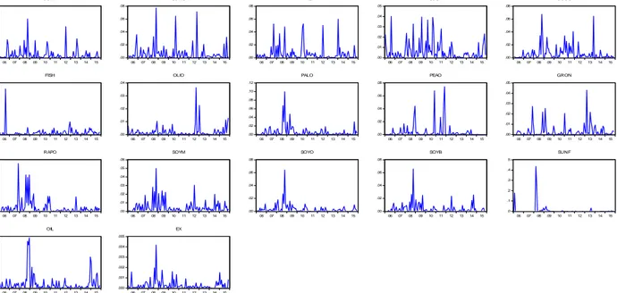
This section presents the results for variance equations of the EGARCH model estimations for both pre- and post-crisis periods2_{. First, this article computed the squared returns for time series and test for evidence of heteroscedasticity and} volatility clustering as our two preconditions for applying EGARCH model. The reason for using the squared returns is originated from the fact that this article cannot reject the hypothesis that the average of the monthly returns is different from zero. If it is assumed that the mean is zero, the unconditional variance can be approximated by the squared returns of the monthly data. The clustering of volatility can be easily observed from the squared returns trend for both pre- and post-crisis

periods in Figure 4 and 5 respectively, which means high (low) volatility tends to be followed by high (low) volatility. .00 .02 .04 .06 .08 .10 86 88 90 92 94 96 98 00 02 04 CORN .00 .04 .08 .12 86 88 90 92 94 96 98 00 02 04 SORG .000 .005 .010 .015 .020 .025 .030 86 88 90 92 94 96 98 00 02 04 WHET .00 .02 .04 .06 .08 .10 86 88 90 92 94 96 98 00 02 04 SUGA .00 .04 .08 .12 .16 86 88 90 92 94 96 98 00 02 04 COCO .00 .01 .02 .03 .04 .05 .06 86 88 90 92 94 96 98 00 02 04 FISH .00 .02 .04 .06 .08 86 88 90 92 94 96 98 00 02 04 OLIO .00 .02 .04 .06 .08 .10 86 88 90 92 94 96 98 00 02 04 PALO .00 .01 .02 .03 .04 86 88 90 92 94 96 98 00 02 04 PEAO .00 .05 .10 .15 .20 .25 86 88 90 92 94 96 98 00 02 04 GRON .0 .1 .2 .3 .4 86 88 90 92 94 96 98 00 02 04 RAPO .00 .02 .04 .06 .08 .10 .12 86 88 90 92 94 96 98 00 02 04 SOYM .000 .004 .008 .012 .016 .020 .024 86 88 90 92 94 96 98 00 02 04 SOYO .00 .02 .04 .06 .08 86 88 90 92 94 96 98 00 02 04 SOYB .00 .02 .04 .06 .08 86 88 90 92 94 96 98 00 02 04 SUNF .00 .04 .08 .12 .16 86 88 90 92 94 96 98 00 02 04 OIL .0000 .0004 .0008 .0012 .0016 .0020 .0024 .0028 86 88 90 92 94 96 98 00 02 04 EX

Figure 4. The Clustering of Volatility from the Squared Returns Trend: Pre-Crisis Period

.00 .02 .04 .06 .08 06 07 08 09 10 11 12 13 14 15 CORN .00 .02 .04 .06 .08 06 07 08 09 10 11 12 13 14 15 SORG .00 .02 .04 .06 .08 06 07 08 09 10 11 12 13 14 15 WHET .00 .01 .02 .03 .04 .05 06 07 08 09 10 11 12 13 14 15 SUGA .00 .02 .04 .06 .08 06 07 08 09 10 11 12 13 14 15 COCO .00 .02 .04 .06 .08 06 07 08 09 10 11 12 13 14 15 FISH .00 .01 .02 .03 .04 06 07 08 09 10 11 12 13 14 15 OLIO .00 .02 .04 .06 .08 .10 .12 06 07 08 09 10 11 12 13 14 15 PALO .00 .02 .04 .06 .08 06 07 08 09 10 11 12 13 14 15 PEAO .00 .01 .02 .03 .04 .05 06 07 08 09 10 11 12 13 14 15 GRON .00 .01 .02 .03 .04 06 07 08 09 10 11 12 13 14 15 RAPO .00 .01 .02 .03 .04 .05 .06 06 07 08 09 10 11 12 13 14 15 SOYM .00 .02 .04 .06 .08 06 07 08 09 10 11 12 13 14 15 SOYO .00 .02 .04 .06 .08 06 07 08 09 10 11 12 13 14 15 SOYB .0 .1 .2 .3 .4 .5 06 07 08 09 10 11 12 13 14 15 SUNF .00 .02 .04 .06 .08 .10 06 07 08 09 10 11 12 13 14 15 OIL .000 .001 .002 .003 .004 .005 06 07 08 09 10 11 12 13 14 15 EX

Figure 5. The Clustering of Volatility from the Squared Returns Trend: Post-Crisis Period

Table 6 presents the results of the volatility estimation through univariate EGARCH modeling in terms of the variance equation for equation (2) in both pre-and post-crisis periods. Most equations were determined to be best fit by AR-EGARCH (1,1). As shown in Table 6, the ARCH parameter (α_i) and the GARCH parameter (β_j) appear to be different across two-time periods. The degrees of volatility persistence, β_j, are statistically significant for all series with exception of soybean oil in the pre-crisis period. Also, the ARCH parameters, α_i are statistically significant for all series with exception of soybeans in the post-crisis period. The absolute values of the degree of volatility persistence, |β_j|, have increased for agricultural commodity prices including corn, sorghum, sugar, coconut, groundnut oil, soybean meal, soybean oil, soybeans, sunflower oil in the post-crisis period. Furthermore, the absolute value of the ARCH parameters, |α_i|, have increased for agricultural commodity prices including corn, wheat, olive oil, palm oil, groundnut oil, rapeseed oil, soybean meal, and sunflower oil for the post-crisis period.

High ARCH parameters imply high short-run volatility, whilst high GARCH parameters indicate high long-run volatility returns (Siami-Namini et al., 2019). The results from the EGARCH model estimations clearly show that the volatility processes of the agricultural commodities return in question is dominated by the ARCH and GARCH effect for two-time periods, but the impact of ARCH and GRACH effect have increased for the post-crisis period. In the other words, more autoregressive persistence in the post-crisis period suggests high long-run volatility in the agricultural commodities. The asymmetric effect parameters, γ_i are significant for all agricultural commodity prices except for corn and soybean

oil for pre-crisis period. Overall, a negative return (or shocks) for the asymmetric effect parameter, γ_i, shows a greater impact on future volatility than positive returns (shocks), and a positive sign shows that a positive shock has a higher impact on future volatility than negative shocks. In the other words, positive and negative shocks have asymmetric effects with positive shocks increasing volatility more than a negative shock (Siami-Namini et al., 2019). For example, corn and soybean oil has a non-significant negative and significant positive return for the pre- and post-crisis period, respectively. This result suggests that corn and soybean oil returns are impacted by positive shocks in the pre- and post-crisis period, but not impacted by negative shocks. As shown in Table 6, crude oil price and U.S. dollar exchange rate have significant positive returns for both periods.

Table 6. Results for Variance Equation

The estimation results of the variance equation of the multivariate AR-EGARCH (1,1) model testing volatility spillover in Equation (4) are presented in Table 7 (Siami-Namini et al., 2018a). As shown in Table 7, most coefficients of the volatility spillovers from crude oil returns to the agricultural commodity returns are significant in the post-crisis period than the pre-crisis period (with exception of corn, and sugar). These results suggest that the volatility of crude oil has a broader impact in the post-crisis period. Furthermore, most coefficients of the volatility spillovers from the U.S. dollar exchange rate to the agricultural commodity returns are significant for pre-crisis period than the post-crisis period. This article concludes that the U.S. dollar exchange rate volatility more strongly impacts the volatility of agricultural commodity returns in the pre-crisis period while the volatility of agricultural commodities returns is highly affected by the volatility of crude oil returns for the post-crisis period.

5.2 The Results of VECM

The Johansen co-integration test shows that there is a long-run relationship between series. Using Schwarz information criterion (SC) for choosing the optimal lag length, this article built several VECM models based on two lags for the pre- and post-crisis periods (Siami-Namini et al., 2018b). Table 8 presents the short- and long-run Granger causality tests based on the VECM approach for pre- and post-crisis periods.

As shown in Table 8, there is no short-run Granger causality from crude oil return volatility to the volatility of the agricultural commodity returns in the pre-crisis period with exception of coconut oil (bidirectional), palm oil (unidirectional) and rapeseed oil (bidirectional), and in the post-crisis period with exception of coconut oil (unidirectional), palm oil (bidirectional), groundnuts (unidirectional), soybean oil (bidirectional). Also, there is unidirectional short-run Granger causality from the GARCH variance series of the sorghum, fishmeal, groundnuts, rapeseed oil, and soybean meal to the crude oil returns volatility in the pre-crisis period. There is unidirectional short-run Granger causality from wheat and rapeseed oil to the crude oil returns volatility in the post-crisis time series.

The results show that there is no short-run Granger causality from the U.S. dollar exchange rate volatility to the volatility of the agricultural commodities returns in the pre-crisis period with exception of coconut oil (unidirectional), soybean meal (unidirectional), and in the post-crisis period with exception of coconut oil (unidirectional), palm oil (bidirectional), groundnuts (bidirectional). Also, there is unidirectional short-run Granger causality from the volatility of fishmeal to the U.S. dollar exchange rates volatility in the pre-crisis period. There is unidirectional short-run Granger causality from the volatility of sugar, groundnut oil, soybean meal, soybean oil, and soybeans to the U.S. dollar exchange rate in the crisis period. These results support previous findings of this article about the existence of large ARCH effects for the post-crisis period than the pre-post-crisis period.

The F-statistic values for long-run causality (the ECT coefficient) are statistically significant for the agricultural commodity returns with exception of palm oil in the pre-crisis period, and are significant for coconut oil, olive oil, palm oil, groundnuts, and soybeans in the post-crisis period. Furthermore, the joint test (for jointly short- and long-run relationships) indicates that there is a strong causality between crude oil returns volatility and all agricultural commodities returns volatility for the pre-crisis period. But, causality between them in the post-crisis period is limited to coconut oil, palm oil, groundnuts, soybean meal, soybean oil, soybeans. Also, the joint test indicates that there is a strong causality between the U.S. dollar exchange rates volatility and agricultural commodities returns volatility with exception of palm oil for the pre-crisis period, and a strong causality for coconut oil, palm oil, groundnuts, and soybeans in the post-crisis period. These results support previous findings of this article about that the crude oil returns volatility (compared to U.S. dollar exchange rate volatility) does strongly affect the volatility of the agricultural commodities returns for the post-crisis period (Siami-Namini et al., 2018c).

Table 8. Continued

*. All figures are the calculated F statistics. P-values are shown in parentheses.

The IRF results for a one standard deviation shock to the crude oil returns volatility and U.S. dollar volatility are presented in Figure 6 and Figure 7 for pre-crisis period, respectively. This article cannot directly compare the magnitudes of the IRFs for two periods. For the pre-crisis period, a positive shock of a one standard deviation increase in the GARCH variance series of crude oil price in Figure 6, leads to immediate declines in corn, sorghum, wheat, fishmeal, palm oil, and soybeans until the second month, followed by increases which return to equilibrium after third or several months. An increase in the crude oil price transmits to the other markets including agricultural market via increases in the production costs.As shown in Figure 7, apositive shock of a one standard deviation increase in the GARCH variance series of exchange rate, leads to immediate declines in corn, sorghum, wheat, coconut, palm oil, groundnut, and soybeans, followed by increases which return to the initial equilibrium after second or several months in the pre-crisis period.

-.000004 -.000002 .000000 .000002 .000004 1 2 3 4 5 6 7 8 9 10 11 12

Response of GCORN to GOIL

-.000006 -.000004 -.000002 .000000 .000002 .000004 1 2 3 4 5 6 7 8 9 10 11 12

Response of GSORG to GOIL

-.000008 -.000006 -.000004 -.000002 .000000 .000002 .000004 1 2 3 4 5 6 7 8 9 10 11 12

Response of GWHET to GOIL

-.0002 -.0001 .0000 .0001 .0002 1 2 3 4 5 6 7 8 9 10 11 12

Response of GSUGA to GOIL

-.000002 -.000001 .000000 .000001 .000002 .000003 .000004 1 2 3 4 5 6 7 8 9 10 11 12

Response of GCOCO to GOIL

-.004 -.002 .000 .002 .004 1 2 3 4 5 6 7 8 9 10 11 12

Response of GFISH to GOIL

-.0000010 -.0000005 .0000000 .0000005 .0000010 .0000015 1 2 3 4 5 6 7 8 9 10 11 12

Response of GOLIO to GOIL

-.0000100 -.0000050 .0000000 .0000050

1 2 3 4 5 6 7 8 9 10 11 12

Response of GPALO to GOIL

-.0000100 -.0000050 .0000000 .0000050 .0000100 1 2 3 4 5 6 7 8 9 10 11 12

Response of GPEAO to GOIL

-1 0 1 2 3 1 2 3 4 5 6 7 8 9 10 11 12

Response of GGRON to GOIL

-.000006 -.000004 -.000002 .000000 .000002 .000004 .000006 1 2 3 4 5 6 7 8 9 10 11 12

Response of GRAPO to GOIL

-.0000010 -.0000005 .0000000 .0000005 .0000010 1 2 3 4 5 6 7 8 9 10 11 12

Response of GSOYM to GOIL

-.0000010 -.0000005 .0000000 .0000005 .0000010 .0000015 1 2 3 4 5 6 7 8 9 10 11 12

Response of GSOYO to GOIL

-.003 -.002 -.001 .000 .001 .002 1 2 3 4 5 6 7 8 9 10 11 12

Response of GSOYB to GOIL

-.0010 -.0005 .0000 .0005 .0010 1 2 3 4 5 6 7 8 9 10 11 12

Response of GSUNF to GOIL

-8.0E-09 -4.0E-09 0.0E+00 4.0E-09 8.0E-09 1 2 3 4 5 6 7 8 9 10 11 12

Response of GEX to GOIL

Response to Cholesky One S.D. Innov ations ± 2 S.E.

-.000004 -.000002 .000000 .000002 .000004 1 2 3 4 5 6 7 8 9 10 11 12

Response of GCORN to GEX

-.000006 -.000004 -.000002 .000000 .000002 .000004 .000006 1 2 3 4 5 6 7 8 9 10 11 12

Response of GSORG to GEX

-.000006 -.000004 -.000002 .000000 .000002 .000004 .000006 1 2 3 4 5 6 7 8 9 10 11 12

Response of GWHET to GEX

-.0001 .0000 .0001 .0002 .0003 1 2 3 4 5 6 7 8 9 10 11 12

Response of GSUGA to GEX

-.000003 -.000002 -.000001 .000000 .000001 .000002 .000003 1 2 3 4 5 6 7 8 9 10 11 12

Response of GCOCO to GEX

-.004 -.002 .000 .002 .004 .006 1 2 3 4 5 6 7 8 9 10 11 12

Response of GFISH to GEX

-.0000010 -.0000005 .0000000 .0000005 .0000010 .0000015 1 2 3 4 5 6 7 8 9 10 11 12

Response of GOLIO to GEX

-.000006 -.000004 -.000002 .000000 .000002 .000004 .000006 1 2 3 4 5 6 7 8 9 10 11 12

Response of GPALO to GEX

-.0000100 -.0000050 .0000000 .0000050 .0000100 .0000150 1 2 3 4 5 6 7 8 9 10 11 12

Response of GPEAO to GEX

-3 -2 -1 0 1 1 2 3 4 5 6 7 8 9 10 11 12

Response of GGRON to GEX

-.000008 -.000004 .000000 .000004 .000008 1 2 3 4 5 6 7 8 9 10 11 12

Response of GRAPO to GEX

-.000001 .000000 .000001

1 2 3 4 5 6 7 8 9 10 11 12

Response of GSOYM to GEX

-.000001 .000000 .000001

1 2 3 4 5 6 7 8 9 10 11 12

Response of GSOYO to GEX

-.0016 -.0012 -.0008 -.0004 .0000 .0004 .0008 .0012 1 2 3 4 5 6 7 8 9 10 11 12

Response of GSOYB to GEX

-.0008 -.0004 .0000 .0004 .0008 .0012 1 2 3 4 5 6 7 8 9 10 11 12

Response of GSUNF to GEX

-.000004 -.000002 .000000 .000002 .000004 1 2 3 4 5 6 7 8 9 10 11 12

Response of GOIL to GEX

Response to Cholesky One S.D. Innov ations ± 2 S.E.

Figure 8 and Figure 9 presents the same effects for the post-crisis period. For the post-crisis period, a positive shock of a one standard deviation increase in the GARCH variance series of crude oil price in Figure 8, leads to immediate declines in corn, sugar, palm oil, groundnut oil, groundnuts, rapeseed oil, soybean meal, soybean oil, and soybeans until the second month, followed by increases which return to equilibrium after third or several months. Also, a positive shock of a one standard deviation increase in the GARCH variance series of exchange rate in Figure 9, leads to immediate declines in corn, fishmeal, olive oil, palm oil, groundnut oil, rapeseed oil, soybean meal, and soybeans, followed by increases which return to the initial equilibrium after second or more months in the post-crisis period.

As a result, the IRF results are not significant for most cases in the pre-crisis period, but they are almost significant in the post-crisis period. This result implies that a shock in the volatility of crude oil returns (GARCH variance series) is not directly transmitted to the volatility of the agricultural commodities returns in the pre-crisis period, but they are directly transmitted in the post-crisis period (Siami-Namini and Hudson, 2016).

-.000008 -.000004 .000000 .000004 .000008 .000012 1 2 3 4 5 6 7 8 9 10 11 12

Response of GCORN to GOIL

-.00004 -.00002 .00000 .00002 .00004 1 2 3 4 5 6 7 8 9 10 11 12

Response of GSORG to GOIL

-.00003 -.00002 -.00001 .00000 .00001 .00002 .00003 1 2 3 4 5 6 7 8 9 10 11 12

Response of GWHET to GOIL

-.00003 -.00002 -.00001 .00000 .00001 .00002 1 2 3 4 5 6 7 8 9 10 11 12

Response of GSUGA to GOIL

-.0000100 -.0000050 .0000000 .0000050 .0000100 1 2 3 4 5 6 7 8 9 10 11 12

Response of GCOCO to GOIL

-.00004 -.00002 .00000 .00002 .00004 1 2 3 4 5 6 7 8 9 10 11 12

Response of GFISH to GOIL

-.00003 -.00002 -.00001 .00000 .00001 .00002 .00003 1 2 3 4 5 6 7 8 9 10 11 12

Response of GOLIO to GOIL

-.00002 -.00001 .00000 .00001 .00002 1 2 3 4 5 6 7 8 9 10 11 12

Response of GPALO to GOIL

-.002 -.001 .000 .001 .002 1 2 3 4 5 6 7 8 9 10 11 12

Response of GPEAO to GOIL

-.0000100 -.0000050 .0000000 .0000050 .0000100 1 2 3 4 5 6 7 8 9 10 11 12

Response of GGRON to GOIL

-.00003 -.00002 -.00001 .00000 .00001 .00002 .00003 1 2 3 4 5 6 7 8 9 10 11 12

Response of GRAPO to GOIL

-.00003 -.00002 -.00001 .00000 .00001 .00002 .00003 1 2 3 4 5 6 7 8 9 10 11 12

Response of GSOYM to GOIL

-.00003 -.00002 -.00001 .00000 .00001 .00002 1 2 3 4 5 6 7 8 9 10 11 12

Response of GSOYO to GOIL

-.000006 -.000004 -.000002 .000000 .000002 .000004 .000006 1 2 3 4 5 6 7 8 9 10 11 12

Response of GSOYB to GOIL

-.0015 -.0010 -.0005 .0000 .0005 .0010 1 2 3 4 5 6 7 8 9 10 11 12

Response of GSUNF to GOIL

-6.0E-08 -4.0E-08 -2.0E-08 0.0E+00 2.0E-08 4.0E-08 6.0E-08 1 2 3 4 5 6 7 8 9 10 11 12

Response of GEX to GOIL

Response to Cholesky One S.D. Innov ations ± 2 S.E.

-.000008 -.000004 .000000 .000004 .000008 1 2 3 4 5 6 7 8 9 10 11 12

Response of GCORN to GEX

-.00002 -.00001 .00000 .00001 .00002 .00003 1 2 3 4 5 6 7 8 9 10 11 12

Response of GSORG to GEX

-.00003 -.00002 -.00001 .00000 .00001 .00002 .00003 1 2 3 4 5 6 7 8 9 10 11 12

Response of GWHET to GEX

-.00003 -.00002 -.00001 .00000 .00001 .00002 .00003 1 2 3 4 5 6 7 8 9 10 11 12

Response of GSUGA to GEX

-.000012 -.000008 -.000004 .000000 .000004 .000008 1 2 3 4 5 6 7 8 9 10 11 12

Response of GCOCO to GEX

-.00006 -.00004 -.00002 .00000 .00002 .00004 1 2 3 4 5 6 7 8 9 10 11 12

Response of GFISH to GEX

-.00004 -.00002 .00000 .00002 .00004 1 2 3 4 5 6 7 8 9 10 11 12

Response of GOLIO to GEX

-.00003 -.00002 -.00001 .00000 .00001 .00002 1 2 3 4 5 6 7 8 9 10 11 12

Response of GPALO to GEX

-.003 -.002 -.001 .000 .001 .002 1 2 3 4 5 6 7 8 9 10 11 12

Response of GPEAO to GEX

-.0000100 -.0000050 .0000000 .0000050 .0000100 1 2 3 4 5 6 7 8 9 10 11 12

Response of GGRON to GEX

-.00003 -.00002 -.00001 .00000 .00001 .00002 1 2 3 4 5 6 7 8 9 10 11 12

Response of GRAPO to GEX

-.00003 -.00002 -.00001 .00000 .00001 .00002 1 2 3 4 5 6 7 8 9 10 11 12

Response of GSOYM to GEX

-.00002 -.00001 .00000 .00001 .00002 1 2 3 4 5 6 7 8 9 10 11 12

Response of GSOYO to GEX

-.000004 -.000002 .000000 .000002 .000004 .000006 1 2 3 4 5 6 7 8 9 10 11 12

Response of GSOYB to GEX

-.0008 -.0004 .0000 .0004 .0008 .0012 1 2 3 4 5 6 7 8 9 10 11 12

Response of GSUNF to GEX

-.00010 -.00005 .00000 .00005 .00010 1 2 3 4 5 6 7 8 9 10 11 12

Response of GOIL to GEX

Response to Cholesky One S.D. Innov ations ± 2 S.E.

Figure 9. Impulse - Response Functions for the Post-Crisis Period Due to One Unit Shock in Exchange Rate Volatility

6. Conclusion

This article examined the relationship between the volatility of the crude oil price and U.S. dollar exchange volatility and the volatility in agricultural commodities prices using monthly data spanning from Jan 1986 to Nov 2015. The selected agricultural commodities are related to the food price index so that the results can help food policy makers understanding the evolving relationship between energy and food prices. The EGARCH model was used to capture spillovers across commodities returns, and then this article extracted GARCH variance series as a measure for volatility of all series. The results showed that the volatility of the agricultural commodities returns was dominated by the ARCH and GARCH effects for the two periods, but the impact of ARCH and GRACH effects have increased for the post-crisis period compared to the pre-crisis period.

This article captured the volatility transmission effects in the crude oil and U.S. dollar exchange rate returns in variance equations. The results showed that volatility in the agricultural commodity returns for most cases are affected by the volatility of the crude oil returns in the post-crisis period. Also, the volatility of the U.S. dollar exchange rate highly affects the agricultural commodities returns in the pre- crisis than the post-crisis periods.

The results of VECM confirm previous findings of this article that there is significant ARCH and GARCH effect between the crude oil returns volatility and U.S. dollar exchange rate volatility and the volatility of the agricultural commodities returns. The ECT coefficient as a measure of long-run relationship between variables in VECM are statistically significant for the agricultural commodity returns with exception of palm oil in the pre-crisis period, and are significant for coconut oil, olive oil, palm oil, groundnuts, and soybeans in the post-crisis period. The joint test showed that there is a strong causality between crude oil returns volatility and all agricultural commodities returns volatility in the pre-crisis period.

But, causality between them in the post-crisis period is limited to coconut oil, palm oil, groundnuts, soybean meal, soybean oil, soybeans. Also, the joint test indicates that there is a strong causality between the U.S. dollar exchange rates volatility and agricultural commodities returns volatility with exception of palm oil for the pre-crisis period, and a strong causality for coconut oil, palm oil, groundnuts, and soybeans in the post-crisis period.

Finally, the IRFs results showed that the crude oil returns volatility does strongly affect the volatility of the agricultural commodities returns in the post-crisis period, and the crude oil returns volatility does affect the volatility of the U.S. dollar exchange rate which in turn influence the volatility of the agricultural commodities returns through changes in the prices. The IRF results are significant for most agricultural commodities volatility in the post-crisis period than the pre-crisis period.

References

Al-Maadid, A., Caporale, G. M., Spagnolo, F., & Spagnolo, N. (2017). Spillovers between Food and Energy Prices and Structural Breaks. International Economics, 150, 1-18. https://doi.org/10.1016/j.inteco.2016.06.005

Alom, F., Ward, B., & Hu, B. (2011). Spillover Effects of World Oil Prices on Food Prices: Evidence for Asia and Pacific countries. In 52nd _{Annual Conference of the New Zealand Association of Economists, 29 June - 1 July 2011.} Balcilar, M., Chang, S., Gupta, R., Kasongo, V., & Kyei, C. (2014). The Relationship between Oil and Agricultural

Commodity Prices: A Quantile Causality Approach, Department of Economics, University of Pretoria.

Cabrera, B. L., & Schulz, F. (2015). Volatility Linkages between Energy and Agricultural Commodity Prices. Energy Economics, 54, 190-203. https://doi.org/10.1016/j.eneco.2015.11.018

Campiche, J., Bryant, H., Richardson, J., & Outlaw. J. (2007). Examining the Evolving Correspondence between Petroleum Prices and Agricultural Commodity Prices. Presentation at the American Agricultural Economics Association Annual Meeting, Portland, OR, and July 29 - Aug 1, 2007.

Cho, G., Kim, M., & Koo, W. W. (2005). Macro Effects on Agricultural Prices in Different Time Horizons, Department of Agribusiness and Applied Economics North Dakota State University. Presentation at the American Agricultural Economics Association Meeting, Providence, Rhode Island, and July 24-27, 2005.

Du, X., Yu, C. L., & Hayes. D. J. (2011). Speculation and Volatility Spillover in the Crude Oil and Agricultural Commodity Markets: A Bayesian Analysis. Energy Economics, 33, 497-503.

https://doi.org/10.1016/j.eneco.2010.12.015

Frank, J., & Garcia, P. (2010). How Strong are the Linkages among Agricultural, Oil, and Exchange Rate Markets? Presentation at the NCCC-134 Conference on Applied Commodity Price Analysis, Forecasting, and Market Risk Management St. Louis, Missouri, April 19-20, 2010.

Frankel, J. A., & Rose, A. K. (2010). Determinants of Agricultural and Mineral Commodity Prices. HKS Faculty Research Working Paper Series RWP10-038, John F. Kennedy School of Government, Harvard University.

Hamao, Y., Masulis, R., & Ng, N. (1990). Correlations in Price Changes and Volatility across International Stock Markets. Review of Financial Studies, 3, 281-307. https://doi.org/10.1093/rfs/3.2.281

Kristoufek, L., Janda, K., & Zilberman, D. (2012). Correlations between Biofuels and Related Commodities before and during the Food Crisis: A Taxonomy Perspective. Energy Economics, 34(5),1380-1391.

https://doi.org/10.1016/j.eneco.2012.06.016

Lu, Y., Yang, L., & Liu, L. (2019). Volatility Spillovers between Crude Oil and Agricultural Commodity Markets since the Financial Crisis. Sustainability, 11, 396. https://doi.org/10.3390/su11020396

Nazlioglu, S., Erdem, C., & Soytas, U. (2013). Volatility Spillover between Oil and Agricultural Commodity Markets. Energy Economics, 36, 658-665. https://doi.org/10.1016/j.eneco.2012.11.009

Nelson, D. B. (1991). Conditional Heteroscedasticity in Asset Returns: A New Approach. Econometrica, 59, 347-370. https://doi.org/10.2307/2938260

Nelson, D. B., & Cao, C. Q. (1992). Inequality Constraints in the Univariate GARCH Model. Journal of Business and Economic Statistics, 10(2), 229-235. https://doi.org/10.1080/07350015.1992.10509902

Perifanis, T., & Dagoumas, A. (2018). Price and Volatility Spillovers between the U.S. Crude Oil and Natural Gas Wholesale Markets. Energies, 11, 2757. https://doi.org/10.3390/en11102757

Rezitis, A. N. (2014). The Relationship between Agricultural Commodity Prices, Crude Oil Prices and U.S. Dollar Exchange Rates: A Panel VAR Approach and Causality Analysis. International Journal of Applied Economics, 29(3). https://doi.org/10.1080/02692171.2014.1001325

Schuh, G. E. (1974). The Exchange Rate and U.S. Agriculture. American Journal of Agricultural Economics, 56, 1-13. https://doi.org/10.2307/1239342

Siami-Namini, S., Hudson, D., Trindade, A., & Lyford. C. (2019). Commodity Price Volatility and U.S. Monetary Policy: Commodity Price Overshooting Revisited. Agribusiness an International Journal, 35(2), 200-218. https://doi.org/10.1002/agr.21564

Siami-Namini, S., Tavakoli, N., & Siami Namin A. (2018a). A Comparison of ARIMA and LSTM in Forecasting Time Series, 2018 17th _{IEEE International Conference on Machine Learning and Applications (ICMLA).} https://doi.org/10.1109/ICMLA.2018.00227

Siami-Namini, S., Muhammad, D., & Fahimullah, F. (2018b). The Short and Long Run Effects of Selected Variables on Tax Revenue - A Case Study. Applied Economics and Finance,5(5), 23-32.

https://doi.org/10.11114/aef.v5i5.3507

Siami-Namini, S., Hudson, D., Trindade, A., & Lyford, C. (2018c). Commodity Prices, Monetary Policy and the Taylor Rule, 2018 Annual Meeting, February 2-6, 2018, Jacksonville, Florida 266722, Southern Agricultural Economics Association.

Siami-Namini, S., & Hudson, D. (2016). U.S. Monetary Policy and Commodities Price Fluctuations. Southern Economic Association - 86th _{Annual Meetings, November 19 - 21, 2016, Washington, DC.}

Strong, N. (1992). Modeling Abnormal Returns: A Review Article. Journal of Business Finance and Accounting, 19(4), 533-553. https://doi.org/10.1111/j.1468-5957.1992.tb00643.x

Theodossiou, P., & Lee, U. (1993). Mean and Volatility Spillovers across Major National Stock Markets: Further Empirical Evidence. Journal of Financial Research, 16, 337-350.

https://doi.org/10.1111/j.1475-6803.1993.tb00152.x

Trujillo-Barrera, A., Mallory, M., & Garcia, P. (2012). Volatility Spillovers in the U.S. Crude Oil, Corn, and Ethanol Markets. Journal of Agricultural and ResourceEconomics, 37(2), 247-262.

Yu, T. H., Bessler, D. A., & Fuller. S. (2006). Co-integration and Causality Analysis of World Vegetable Oil and Crude Oil Prices. Presentation at the American Agricultural Economics Association Annual Meeting, Long Beach, CA, and July 23-26, 2006.

Zafeiriou, E., Arabatzis, G., Karanikola, P., Tampakis, S., & Tsiantikoudis, S. (2018). Agricultural Commodities and Crude Oil Prices: An Empirical Investigation of Their Relationship. Sustainability, 10, 1199.

https://doi.org/10.3390/su10041199

Zhang, Z., Lohr, L., Escalante C., & Wetzstein, M. (2010). Food versus Fuel: What Do Prices tell us? Energy Policy, 38: 445-451. https://doi.org/10.1016/j.enpol.2009.09.034

Copyrights

Copyright for this article is retained by the author(s), with first publication rights granted to the journal.

This is an open-access article distributed under the terms and conditions of the Creative Commons Attribution license which permits unrestricted use, distribution, and reproduction in any medium, provided the original work is properly cited.