econ
stor
www.econstor.eu
Der Open-Access-Publikationsserver der ZBW – Leibniz-Informationszentrum Wirtschaft
The Open Access Publication Server of the ZBW – Leibniz Information Centre for Economics
Nutzungsbedingungen:
Die ZBW räumt Ihnen als Nutzerin/Nutzer das unentgeltliche, räumlich unbeschränkte und zeitlich auf die Dauer des Schutzrechts beschränkte einfache Recht ein, das ausgewählte Werk im Rahmen der unter
→ http://www.econstor.eu/dspace/Nutzungsbedingungen nachzulesenden vollständigen Nutzungsbedingungen zu vervielfältigen, mit denen die Nutzerin/der Nutzer sich durch die erste Nutzung einverstanden erklärt.
Terms of use:
The ZBW grants you, the user, the non-exclusive right to use the selected work free of charge, territorially unrestricted and within the time limit of the term of the property rights according to the terms specified at
→ http://www.econstor.eu/dspace/Nutzungsbedingungen By the first use of the selected work the user agrees and declares to comply with these terms of use.
Lengnick, Matthias; Wohltmann, Hans-Werner
Working Paper
Agent-based financial markets and
New Keynesian macroeconomics: A
synthesis
Economics working paper / Christian-Albrechts-Universität Kiel, Department of Economics, No. 2010,10
Provided in cooperation with:
Christian-Albrechts-Universität Kiel (CAU)
Suggested citation: Lengnick, Matthias; Wohltmann, Hans-Werner (2010) : Agent-based financial markets and New Keynesian macroeconomics: A synthesis, Economics working paper / Christian-Albrechts-Universität Kiel, Department of Economics, No. 2010,10, http:// hdl.handle.net/10419/41552
agent-based financial markets and
new keynesian macroeconomics
-a
synthesis-by Matthias Lengnick and Hans-Werner Wohltmann
No 2010-10Agent-Based Financial Markets and
New Keynesian Macroeconomics
– A Synthesis –
Matthias Lengnick
∗University of Kiel
University of Mannheim
Hans-Werner Wohltmann
∗∗University of Kiel
November 4, 2010
AbstractWe combine a simple agent-based model of financial markets with a standard New Keynesian macroe-conomic model via two straightforward channels. The result is a macroemacroe-conomic model that allows for the endogenous development of stock price bubbles. Even with such a simplistic comprehensive model, we can show that the behavioral foundations of the stock market exert important influence on the macroeconomy, e.g. they change the impulse-response functions of macroeconomic variables significantly. We also analyze financial market transaction taxes as well as asset price bubble de-flating monetary policy, and find that both can be used to reduce volatility and distortion of the macroeconomic aggregates.
JEL classification: E0, E52, G12, G18
transac-Economists [...] have to do their best to incorporate the realities of finance into macroeconomics.
Paul Krugman (2009)
1 Introduction
The economies of almost every country have recently been hit by a turmoil in the financial markets. This so-called financial crisis has vividly demonstrated that developments in the financial markets can have major impacts on the real economy. Interdependencies between real and financial markets should therefore obviously be taken into account when doing macroeconomics. Natural questions to ask are: to which extent the formation and bursting of bubbles spills over into real markets, and whether financial market regulation can reduce disturbances of the real markets.
For about two decades now, a relatively new modeling approach has been applied to the analy-sis of financial and foreign exchange markets. This approach builds on the method of agent-based computational (ABC) simulation, it drops the assumptions of rational expectations, homogeneous individuals, perfect ex ante coordination and often also market equilibria, in favor of adaptive learn-ing, simple interactions of heterogeneous agents, and emerging complex macroscopic phenomena.1 The approach seems very promising thus far since, on the one hand, it is grounded in the results of survey studies2 and laboratory experiments3, and on the other hand, the emerging macro-dynamics mimic the properties of real world data (such as martingale property of stock prices, fat tails of return distribution, volatility clustering and dependency in higher moments)4 quite well, a success that traditional financial market models, building on equilibrium and rationality, do not provide.5 A huge literature has already developed on this topic that – despite its success – is largely ignored by macroeconomists.
One strength of the ABC method is that it naturally allows for the endogenous emergence of bubbles. In such models, investors can typically choose from a set of different non-rational trading 1 For an introduction into ABC financial market modeling see, e.g., Samanidou et al. (2006), Hommes (2006) or LeBaron
(2006). Outstanding examples of such models are Kirman (1993), Brock and Hommes (1998), and Lux and Marchesi (2000).
2 Frankel and Froot (1987), Ito (1990), Taylor and Allen (1992), Lui and Mole (1998). 3
Caginalp et al. (2001), Sonnemans et al. (2004), Hommes et al. (2005).
4 A detailed description of thesestylized factscan be found in Lux (2009). 5
De Grauwe and Grimaldi (2006), for example, compare the performance of an agent-based model with popular models like that of Obstfeld and Rogoff in explaining the stylized facts of foreign exchange rates. They find that the former performs much better.
strategies. A continuous evaluation of those strategies according to past performance leads to changes in the size of the different investor groups. In phases that are dominated by technically operating investors, stock prices can deviate sharply from their underlying fundamental value. If market sentiments change and fundamentalists dominate, convergence towards the fundamental value sets in. Inspired by the spectacular failure of mainstream macroeconomics to provide an explanation of the current crisis and an agenda of how to deal with it, a number of authors are calling for the use of ABC models in macroeconomics.6
The emergence of asset price misalignments (i.e. bubbles) on the financial markets is often seen as having the most devastating impact on the real economy. Some macroeconomic models already allow for such misalignments. Bernanke and Gertler (1999), for example, augment the model of Bernanke et al. (1999) by imposing an exogenously given path for asset price misalignment. In their model, each bubble has a constant exogenous probability to burst, where ”burst” simply means that asset prices immediately return to their fundamental value. Kontonikas & Ioannidis [KI] (2005) and Kontonikas & Montagnoli [KM] (2006) use forward- and backward-looking New Keynesian macroeconomic (NKM) models with lagged stock wealth effects. The stock price dynamics in these models are not exogenously imposed and the crash of a bubble does not simply occur with a fixed probability. Instead they make use of an endogenous dynamic process that binds stock prices to two different forces: One of which leads to a return towards the fundamental value, and the other – so-called momentum effect – relates stock prices to their own past development. While KI (2005) and KM (2006) are clearly inspired by the agent-based financial markets literature with its fundamentalist and chartist trading rules, none of the above models explicitly motivates the dynamics of stock price misalignment by boundedly rational investor behavior and none makes use of an endogenous learning or evaluation mechanism.
In a recent paper Bask (2009) uses a New Keynesian dynamic stochastic general equilibrium (DSGE) framework with stock prices that are determined by the demand of two different types of investors: chartists and fundamentalists. While the model provides the major advantage that it justifies stock price movements by the behavior of these two types of investors, it does not allow for an endogenous evaluation of the different investment strategies. Investors therefore keep employing 6
See, e.g., Colander et al. (2008), Colander et al. (2009), Lux and Westerhoff (2009), Krugman (2009), Kirman (2010), Delli Gatti et al. (2010), and Dawid and Neugart (forthcoming). Examples of purely agent-based macro models (with no connection to NKM) are Gaffeo et al. (2008) or Deissenberg et al. (2008).
the same investment rule and do not try to learn from past price developments. Thus, the model misses an important aspect of financial market dynamics. Milani (2008) and Castelnuovo and Nistico (2010) have integrated stock price misalignment into a New Keynesian DSGE model. Their aim is to provide insights into the dynamics of the stock price component that is driven by utility-optimizing, rational-expecting agents.
In this paper, we connect a simple ABC model of financial markets with the baseline New Keyne-sian DSGE model, which is purely forward-looking. To the best of our knowledge, no such attempt has been made so far. Since we combine two separate subdisciplines of economics, and do not want to exclude readers who are not familiar with both of these areas, our approach focuses on simplicity. Nonetheless, our model leads to a number of interesting insights. We find that stock market de-velopments, which are more realistically described by the termanimal spirits than rationality, may have strong impacts on the real economy. The history dependence property of financial markets carries over to the real sector. We also find that the negative impact that speculative behavior of financial market participants exerts on the macroeconomy, can be reduced by the introduction of a transaction tax. Our results further suggest that monetary policy can be used to control the spillover of financial market fluctuations into the real sector. And that a bubble-deflating policy could reduce volatility or distortion of the real economic variables.
The model is developed in section 2. We analyze the interaction between real and financial markets by means of numerical simulation in section 3. Policy related issues like the impact of a financial transaction tax and an augmented Taylor-rule are discussed in section 4. Section 5 concludes.
2 The Model
Our model consists of two parts, one describing the financial sector, and one the real sector of the economy. We use the ABC chartist-fundamentalist model proposed by Westerhoff (2008) to model the financial market. The real sector is described by the NKM framework in its basic notation augmented by a cost effect of stock prices. Since we allow for an endogenous development of animal spirits and bubbles, our model is an augmentation of NKM models that already include stock price bubbles, but impose their dynamics exogenously (see above). It is also an augmentation of those models that integrate a stock market with different types of investors into macroeconomics, but do not employ endogenous learning. Our approach is complementary to models that incorporate stock
markets (via total micro foundation) completely into a DSGE world because stock price gaps are driven by behavioral rules, and do not result from rigidities.7 It is also complementary to models that incorporate behavioral rules (animal spirits) into the real sector of macroeconomic models.8 The model is implemented in Matlab.9
The first problem one has to deal with is that the rules determining the dynamics of financial markets are likely to be very different from those of the real markets. First, economic transactions in the former seem to take place much more frequently than in the latter,10 implying that both can not be modeled on the same time scale.11 Second, the Efficient Market Hypothesis (EMH) as put forward by Fama (1965) suggests that future developments are much harder to predict for financial time series than for real ones. This argument implies that differing expectation formations should be used in the two parts of the model.
The two modeling methodologies employed throughout this paper are very different in nature. In order to allow for the different methods of analysis that are common in ABC and DSGE modeling, we do not simply integrate one into the other, but take the differences seriously. As a result, we must assume that real and financial markets are populated by different kinds of agents. We interpret those of the financial market to be institutional investors, who have the resources to participate in high frequency trading. Conversely, real market agents have neither detailed knowledge about financial markets, nor the possibility to participate in high frequency trading. Subsection 2.1 defines the financial sector of our economy, while 2.2 defines the real one. Subsection 2.3 brings the two sectors together.
2.1 Financial Market
We use the model proposed by Westerhoff (2008) to define the financial sector of our economy for two reasons: First, because of its straightforward assumptions and easy implementation, and second, because it has already often been used for policy analysis (especially transaction taxes) so that its
7
See, e.g., the already cited papers of Milani (2008) and Castelnuovo and Nistico (2010).
8 See, e.g., the recent Paper by De Grauwe (2010). 9
The source code is available upon request.
10Although this argument seems to be straightforward it is also backed empirically by Aoki and Yoshikawa (2007), who
find that time series of real economic data do not share the power law distribution of financial markets which implies that the latter are characterized by higher economic activity.
11
behavior in this respect is well known.12 In this model, stock price adjustment is given by a price impact function:
st+1 =st+a WtCDCt +WtFDFt
+st (1)
DC and DF stand for the orders generated by chartists and fundamentalists, respectively.13 WC
andWF denote the fractions of agents using these strategies, andais a positive reaction parameter. Eq. (1) can be interpreted as a market maker scenario, where prices are adjusted according to observed excess demand.14 Since fundamentalist and chartist investment strategies do not account for all possible strategies that exist in real markets, a noise terms is added that is i.i.d. normally distributed with standard deviation σs. It could be interpreted as the influence of those other strategies. t denotes the time index which is interpreted as days. For the sake of simplicity, we assume that the true (log) fundamental value of the stock price ¯sf equals zero. Thus, the stock price
st also equals the stock price misalignment.
Chartists expect that the direction of the recently observed price trend is going to continue: ECt [st+1−st] =kC[st−st−1] (2)
kC is a positive parameter that denotes the strength of trend extrapolation. Fundamentalists, on the other hand, expect that kF ·100 % of the actual perceived mispricing is corrected during the next period: EFt [st+1−st] =kF h sft −st i (3)
sft is the perceived fundamental value that does not necessarily equal its true counterpart ¯sf. The
12The approach is, for example, also used in Westerhoff and Dieci (2006) who model two financial markets and their
interaction when introducing transaction taxes. Demary (2010) also analyzes the effects of introducing such taxes in a basic Westerhoff-model augmented by different time horizons of investors.
13
Negative orders denote a supply of stock.
14
There are also agent-based financial models that make use of Walrasian market clearing. See for example Brock and Hommes (1998).
difference between sft and ¯sf is explained in detail in subsection 2.3. Assuming that the demand generated by each type of investors depends positively on the expected price development leads to:
Dit=`Eit[st+1−st] +it i={C, F} (4)
` is a positive reaction parameter. Since (2) and (3) do not reflect the great amount of chartist and fundamentalist trading strategies that exist in real world markets, the noise termit is added. It is normally distributed with standard deviation σi and can be interpreted as the influence of all other forecasting strategies different from (2) and (3). The demand generated by chartist and fundamentalist trading rules is therefore given by:15
DtC =b(st−st−1) +Ct b=`·kC (5)
DtF =csft −st
+Ft c=`·kF (6) The fractions of agents using the two different investment strategies are not fixed over time. Instead, agents continuously evaluate the strategies they use according to past performance. The better a strategy performs relative to the other, the more likely it is that agents will employ it. It is assumed that the attractiveness of a particular strategy depends on its most recent performance (exp{st} −exp{st−1})Dit−2 as well as its past attractivenessAit−1:16
Ati = (exp{st} −exp{st−1})Dti−2+dAit−1 i={C, F} (7)
The memory parameter 0 ≤ d ≤ 1 defines the strength with which agents discount past profits. The extreme casesd= 0 and d= 1 relate to scenarios where agents have zero and infinite memory. Note the timing of the model: Orders submitted in t−2 are executed int−1. Their profitability ultimately depends on the price realization in t. Agents may also withdraw from trading (strategy
15Westerhoff (2008) directly assumes eq. (5) and (6) and does not explicitly state the different types of expectation
formations.
16Recall thats
“0”). The attractiveness of this strategyA0t is normalized to zero A0t = 0. The fraction of agents that employ strategyiis given by the well knowndiscrete choice orGibbs probabilities:17
Wti = exp{eA
i t}
exp{eAC
t }+ exp{eAFt }+ exp{eA0t}
i={C, F, 0} (8)
The more attractive a strategy, the higher the fraction of agents using it. Note that the probability of choosing one of the three strategies never becomes negative. The positive parameter emeasures the intensity of choice. The higher (lower) e, the greater (lesser) the fraction of agents that will employ the strategy with the highest attractiveness. This parameter is often called therationality parameter in ABC financial market models.18 The only difference between our financial market submodel and that of Westerhoff (2008) is that we distinguish between the true fundamental value ¯
sf and the trader’s perception of it,sft. Both models are equivalent if sft = ¯sf.
2.2 Real Markets
The partial model describing the real sector is given by a simple modification of the baseline NKM model. New Keynesian models are widely used in macroeconomics because they typically allow for a good fit of real world data, and they are derived from individual optimization so that both its parameters and shocks can argued to be structural. The model consists of the following three equations: iq =δππq + δxxq (9) xq = Eq[xq+1] − 1 σ(iq−Eq[πq+1]) (10) πq =βEq[πq+1] + γxq − κsq + πq (11)
The notation of the variables is as follows: i is the deviation of the nominal interest rate from its target,π the deviation of the inflation rate from its target,x the (log) output gap (i.e. its deviation from steady state), and sthe deviation of the (log) nominal stock price from its true fundamental value ¯sf. The subscript q= 1, ..., Qdenotes the time index. We keep the common interpretation of the time index in New Keynesian models and assume that it denotes quarters. Eqis the expectations
17See, e.g., Manski and McFadden (1981) for a detailed explanation of discrete choice models. 18
operator conditional on knowledge available inq. The dynamic path of the stock pricesis determined exogenously to the real sector by the model developed in 2.1.
Equation (9) is a standard monetary policy interest rule. The central bank reacts to deviations of inflation and output from its target. Equation (10) is referred to as the dynamic IS-curve that describes the demand side of the economy. It results from the Euler equation (which is the result of intertemporal utility maximization) and market clearing in the goods market. Equation (11) is a New Keynesian Phillips curve that represents the supply side. It can be derived under the assumptions of nominal price rigidity and monopolistic competition. Asset prices influence the economy through a
balance sheet channel that works as follows: The willingness of banks to grant credits might depend on the borrowers’ financial position. For example, agents could use assets they hold as collateral when borrowing money. The more collateral the debtor has to offer, the more advantageous his credit contract will be. In this context, “advantageous” may mean that either credits of larger size are offered or that credits of the same size could be obtained cheaper (lower interest payments). The first argument can be used to relate asset prices positively to aggregate demand, as for example done in Bernanke and Gertler (1999), Kontonikas and Ioannidis (2005), Kontonikas and Montagnoli (2006), or Bask (2009). We stress the second argument in this paper. Higher prices of assets owned by firms increase their creditworthiness, and allow them access to cheaper credits. Since most firms’ production is largely financed through credits, asset prices are inversely related to firms marginal (real) costs of production. This argument allows the addition of the term−κsq to equation (11).19
This verbal kind of micro foundation is sufficient for our purposes. The reader is referred to Bernanke and Gertler (1999) who discuss a balance sheet channel (and its microfoundation) in more detail. The variableπq is a stochastic element with zero mean.
To derive eq. (10), it is commonly assumed that the household’s only possibility of transferring wealth into future periods is by demanding bonds. Households therefore do not hold or trade stock. We keep this assumption in order to allow for analysis of the isolated impact of the speculation of 19
Note that we defined sq as the nominal stock price gap. The so-called cost channel of monetary transmission is
commonly introduced into New Keynesian models via the nominal interest rate (see for example Ravenna and Walsh (2006)). Analogously to this channel, we also decided to insert the nominal (and not the real) stock price gap into (11). Note also that our definition of the stock price gap is very different from that of Milani (2008) or Castelnuovo and Nistico (2010), who define it as the difference between the stock price under fully flexible and somewhat rigid market conditions. Both, of course, are the result of utility optimal paths under rational expectations.
ABC financial market models could also be employed for the analysis of foreign exchange rates. Since a rise (fall) of foreign exchange rates would also raise (lower) production costs – via more expensive (cheaper) intermediate inputs – they would be included with the opposite sign (i.e. +κsq). To avoid confusion, we mention explicitly that we are
financial market participants on stock prices. We further assume that firms hold an initial amount of stock but do not participate in stock trading. Consequently, they are only affected by the financial sector via the balance sheet channel, and not via speculative gains. The financial sector can not generate profits on the aggregate level by selling and reselling stock. If one agent wins from a beneficial transaction, others must lose. The only possibility for the aggregate stock market to earn profits is by dividend payments from the real sector. Because they are relatively small in size, and because the Westerhoff-model does not explicitly take financial wealth into account, we do not model the stream of dividend payments from firms to financial investors. As a result of the above assumptions, financial streams between the real and financial sector do not exist.
The model in reduced form writes as follows:
1 +δx σ δπ σ −γ 1 | {z } A xq πq = 1 σ1 0 β | {z } B Eq[xq+1] Eq[πq+1] + 0 −κ sq+ 0 1 πq (12)
The dynamics of the forward-looking variables x and π depend on the current value of s as well as the expectations of their future values. Therefore, x and π are also indirectly dependent on the expected future development of s. We assume that those expectations about the future stock price are formed in a stationary way:
Eq[sq+k] =sq ∀k= 1, 2, ... (13)
The usage of non-rational expectations has often been criticized in macroeconomics. However, we find that it is much more unrealistic to assume that future asset price movements could be known ex ante. Instead, it is reasonable to assume that real-market agents can generally be described as non-experts regarding knowledge about future stock price developments, and that they do not bet on trend extrapolation or mean reversion. We decided to model the real market agents as EMH-believers for the sake of simplicity and because – following Fama (1965) – this kind of expectation formation can be considered the most rational that is possible.20
At the same time, we find it unreasonable to model the expectations about quarterly real variables in the same way as those of high frequency financial markets. Thus the expectations of output and 20
inflation are formed rationally with respect to the non-rational expectations ofsq, i.e., as rational as
possible given the uncertain development ofsq: Agents know the mean realization of future x and
π that would result if (13) is on average correct.
If sq is exogenously given and non-explosive, xq and πq can be calculated via forward-solution
as:21 xq πq = (A−B) −1 0 −κ sq+A−1 0 1 πq (14)
We take a closer look on the implications that the interaction of financial and real markets has for the stability of the system in the next subsection. The nominal interest rate can then be calculated by eq. (9) and the real interest rate by:
iq−Eq[πq+1] =σ(Eq[xq+1]−xq) (15)
2.3 Bringing the Two Sectors Together
As already mentioned, the two parts of the model run on different time scales. The real markets operate quarterly while the financial market operates daily. We assume that one quarter consists of 64 trading days. Therefore, the financial sector performs 64 increments of the time indext within one increment of the real market’s time indexq (figure 1). Quarterq is defined to contain the days 64(q−1) + 1, ...,64q.
t: 123 ... 64 65 ... 128
q: 1 2
Figure 1: Time scale as indexed by days (t) and quarters (q)
We assume that the relevant value of the quarterly stock pricesq that affects xq and πq via eq.
21
Of course the parameters must be selected in a way that the Blanchard-Kahn condition holds. In the case of the NKM, it is sufficient thatδx≥0,δπ>1.
Real
Markets FinancialMarket
Channel I: Cost Effect
Channel II: Misperception Effect
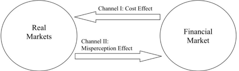
Figure 2: Channels between real and financial markets
(14) is the average of the daily realizations of st of the corresponding quarter q. Thus sq is given
by:22 sq = 1 64 64q X t=64(q−1)+1 st (16)
Using the definitions above, we calculate the recursive dynamics of the financial market for one quarter q (in days: t = (q−1)·64 + 1 , ... , q·64) with the agent-based model defined in section 2.1, and insert the mean of the resultingst’s into eq. (14) in order to calculate the NKM’s reaction.
Note that the mean value sq is determined after all corresponding daily values ofst are calculated.
Since expectations about the future development of quarterly stock prices are formed in a stationary manner,sq is indeed exogenous to the dynamic process (12) so that the forward solution (14) holds.
Now that we have set up the real and financial markets we are able to define the difference between the true fundamental stock price (¯sft) and the fundamentalist’s perception of it (sft). The fundamental value of any given stock is commonly understood to be the sum of all discounted future dividend paymentsdt+k: sft = ∞ X k=1 ρk Et[dt+k] (17)
Dividends are typically closely related to real economic conditions (xq in our model). Therefore,sft
would depend on the expectation ofx for all future days. We decided to model the perception of the fundamental value in a different way for two reasons: First, it has been empirically found that stock markets overreact to new information, i.e. stock prices show stronger reactions to new information 22Equation (16) assumes that the influence of daily stock prices on the real economy is equal for each day in the quarter.
than they should, given that agents behave rationally.23 Second, it has been argued that in reality it is very difficult (if not impossible) to identify thetruefundamental value of any stock.24 Given these problems, it seems reasonable to assume that agents do not know the true value of ¯sf or calculate it in a rational way (as in eq. (17)), but instead simply take the current development of the real economy as a proxy for it.
sft =h·xq q= floor t−1 64 , h≥0 (18)
The floor-function rounds a real number down to the next integer. Eq. (18) states that the funda-mentalists’ perception sft is biased in the direction of the most recent real economic activity, i.e., if output is high (low) the fundamental stock price is perceived to lie above (below) its true coun-terpart. Note that ABC models of financial markets typically can not relate the fundamental value to recent economic development, since the latter is not modeled endogenously. Most models do not distinguish betweensft and ¯sf, they set both equal to zero or assume them to follow a random walk.25 Figure 2 illustrates the two channels that exist between the real and the financial market. Channel I (the cost channel) allows the financial market to influence the real sector and disappears if
κin eq. (11) is set equal toκ= 0. Channel II (the misperception of ¯sf channel) allows for influence in the opposite direction, and disappears ifh is set equal to h = 0. If both of these cross-sectoral parameters are set equal to zero (κ = 0 & h = 0), both sectors (i.e. both submodels) operate independently of each other.
The stability condition of the real sector is independent ofκandh. An explosive path forxqcould
only be the result of an explosive path of st. The two cross-sectoral channels feed on each other:
If stock prices are high, Channel I exerts a positive influence on output. Output rises, which in turn exerts a positive influence on stock prices through Channel II, and so on. To exclude explosive paths,κ (h) has to be lower, the higherh (κ) is. Figure 3 shows a numerical approximation of the stability region inh-κ-space.26
The steady state of the NKM submodel in isolation (for κ = 0) is given by x = 0, π = 0 and
23De Bondt and Thaler (1985) were among the first to describe this phenomenon. 24
For example Rudebusch (2005) or Bernanke and Gertler (1999) raise doubts of this kind.
25
Again, Westerhoff (2008) is a good example to look at since both of these approaches are discussed there.
26
0 0.5 1 1.5 2 0 0.2 0.4 0.6 0.8 1 h κ Stable Region Unstable Region
Figure 3: Stability region of κ andh
i = 0. If κ 6= 0 this steady state could only be reached, if the stock price equals its fundamental value (sq = 0). We call a state in whichx= 0,π= 0,i= 0 andsq= 0 thefundamental steady state.
3 Numerical Simulations
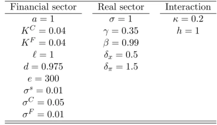
The analysis of our model is performed by means of numerical simulation. The calibration is given in Table 1. The parameter values for the real sector are common in macroeconomic analysis, those of the financial sector are exactly the same as in Westerhoff (2008). In order to set the cross-sectoral parameters, we assume that the real sector is much less influenced by the financial sector than the other way round.27 Therefore we set h to be five times larger thanκ.
Table 1: Baseline Calibration of the Model Financial sector Real sector Interaction
a= 1 σ = 1 κ= 0.2 KC = 0.04 γ = 0.35 h= 1 KF = 0.04 β = 0.99 `= 1 δx= 0.5 d= 0.975 δπ = 1.5 e= 300 σs= 0.01 σC = 0.05 σF = 0.01 27
It is known that stock prices overreact to new information. Since new information in our case is assumed to be the development of the real sector, this argument implies a strong reaction of s to x. See, e.g., De Bondt and Thaler (1985), Nam et al. (2001), or Becker et al. (2007), and references therein.
3.1 Financial Sector Disturbances
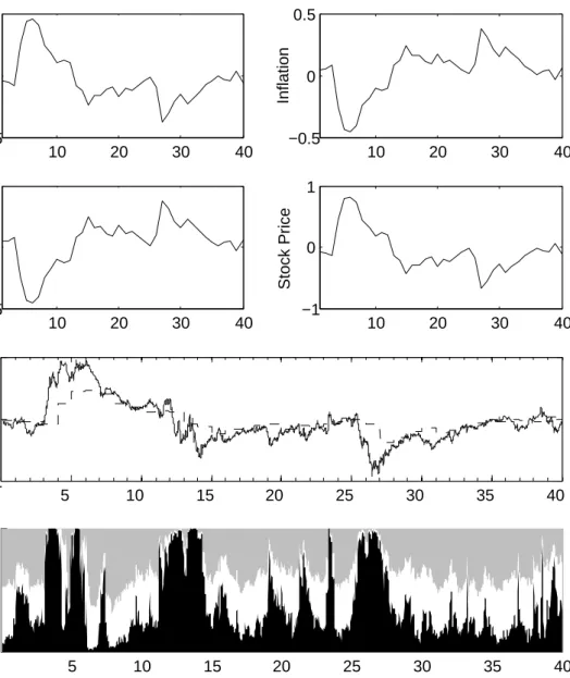
To demonstrate the working of our model, we perform one “representative” run. The simulated time period consists of 40 quarters or 2560 days. Both parts of the model contain noise. However, the practical implementation of these noise terms in ABC financial market models differs from that in New Keynesian DSGE models. The former typically analyze the response of the system (12) resulting from one exogenously imposed realization of the noise termπq under the assumption that all other realizations ofπq are zero. The latter, in contrast, repeatedly draw realizations of the noise terms from pseudo random number generators. For our simulation, we take these methodological differences seriously and employ each method for the respective sector. In this subsection we draw realizations for noise terms from the financial sector while keeping the noise term of the real sector equal to zero. Figure 4 shows the resulting dynamics for xq, πq, iq, sq, st, and a variable called animal spirits. The latter represents the fraction of agents, employing the three trading strategies. Black denotes chartist trading, gray fundamentalist trading, and white no trading.28 The horizontal time axes are quarterly scaled. In the diagrams containing daily data, quarters cover an interval containing 64 data points.
The model generates endogenous waves of chartism and fundamentalism. Each strategy is able to dominate the market from time to time, but the endogenous competition between them assures that neither dominates forever. In phases dominated by chartists (e.g., q = 4−6 or 26−28), the stock price departs largely from its fundamental value, i.e., a bubble builds up. If the market is dominated by fundamentalists (e.g.,q= 7−10 or 32−36), the stock price returns to its fundamental value.
Although no exogenous shock (through π
q) acts on the real sector, it is subject to considerable
change. If quarterly stock prices are high (low), the output gap is also high (low), while inflation and interest rates are low (high). The economic variables of the real sector return to their respective fundamental steady state only if fundamentalists dominate the financial market. Stock prices are much smoother on a quarterly basis than on a daily one: Real markets are influenced by quarterly stock prices, so that the influence of daily stock price fluctuations does not spill over into the real sector.
28In a recent paper, De Grauwe (2010) introduces non-rational expectation formation into an otherwise standard NKM
model. In his model, De Grauwe calls the non-rational spontaneous formation of optimism and pessimism concerning expectations of future output and inflation animal spirits. In our model, the expression is used to denote non-rational investor behavior on the stock market, while real market expectations are not subject to any form of animal spirits.
10 20 30 40 −0.5 0 0.5 Outputgap 10 20 30 40 −0.5 0 0.5 Inflation 10 20 30 40 −0.5 0 0.5 Interest Rate 10 20 30 40 −1 0 1 Stock Price 5 10 15 20 25 30 35 40 −1 0 1
Stock Price (daily)
5 10 15 20 25 30 35 40
0 0.5 1
Animal Spirits (daily)
Figure 4: Model Output for a Time Period ofQ= 40
Writing (14) separately for xq and πq under the assumption that no shocks from the real sector
occur (π q = 0 ∀q) gives: xq = 1 ∆(δπ−1)κsq with ∆ = (δπ−1)γ+δx(1−β) (19) πq =− 1 ∆δxκsq (20)
Since ∆1 (δπ−1) > 0 and −∆1δx < 0 the stock price exerts a proportional positive influence on
The monetary policy parameters δx and δπ can be used to control the spillover of financial market
disturbances onx and π. Dividing (19) by (20) gives the relation betweenxq andπq:
xq πq =−δπ−1 δx ⇔ xq= 1−δπ δx πq (21) Because 1−δπ
δx = 1 in our parameterization, (21) reduces toxq =−πq. The interest rate is calculated
by inserting (21) into (9):
iq=δππq + δx
1−δπ
δx
πq ⇔ iq=πq (22)
We do not show the time paths for the real interest rateiq−Eq[πq+1], since it equals zero for all
quartersq. If the error term from the real sector equalsπq = 0 for any periodq, there is no difference betweenxq and Eq[xq+1] that can be expected (a fact that follows directly from eq. (13) and (19)).
Eq[xq+1] =xq implies that the real interest rate equals zero (see eq. (15)). It can only deviate from
zero if a difference between xq and Eq[xq+1] exists, i.e. if πq 6= 0. Similar considerations lead to
Eq[πq+1] =πq for the inflation rate. In the above simulation, changes ofxq andπqnonetheless occur
since they are driven by the stock market via unexpected changes in sq (see eq. (19) and (20)).
The above equations show that the transmission of disturbances from the financial to the real sector is still rather simple. In fact, if shocks from the real sector are not considered, all real variables change in linear proportion to the stock price. One consequence is that the generated quarterly time paths all have the same empirical kurtosis of about 9. While excess kurtosis (> 3) is one of the stylized facts of financial markets, it seems to be unrealistic for real markets since it implies that the occurrence of extreme events (like a drop of stock price by more than 20%) is equally likely for both kinds of markets. Future work should focus on the question of how the spillover of distributional properties from the financial to the real markets could become more realistic in this respect.29
3.2 Real Sector Disturbances
In this subsection, we take the other point of view and analyze the effects of an exogenous shock of the real sector. In DSGE models, such questions are typically analyzed via impulse response functions that try to isolate the effects of an exogenous realization of the stochastic termπq. We are 29
0 10 20 30 −0.8 −0.6 −0.4 −0.2 0 Outputgap 10 20 30 −0.8 −0.6 −0.4 −0.2 0 Stock Price 0 10 20 30 0 0.2 0.4 0.6 0.8 Inflation 0 10 20 30 0 0.2 0.4 0.6 0.8
Real Interest Rate
Figure 5: Mean response to a cost shock with both channels active. The dashed lines give the 95 % confidence band.
interested in the impact of an unanticipated, transitory cost shock without persistence, i.e. π5 = 1. In order to allow for impulse response analysis in a way similar to that typically used in DSGE models, we perform the following experiment:
1. Generate the model dynamics withπq = 0 for all q.
2. Generate the same dynamics with identical realizations of the pseudo random numbers, but withπ5 = 1.
3. Calculate the differences of the trajectories of step 1 and 2 which gives the isolated impact of the cost shock. Note that the noise terms are identical in both runs.
4. Repeat steps 1-3 10,000 times.
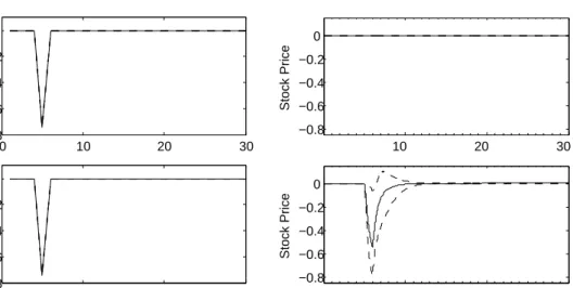
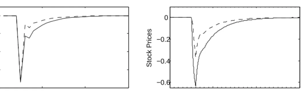
Figure 5 shows the resulting responses to an exogenous shock ofπ5 = 1 for our baseline calibration. The solid lines illustrate the mean responses, while the dashed lines represent 95% quantiles. The economy shows the typical stagflationary response to the cost shock. Inflation and the real interest rate rise, while output and the stock price fall. We repeat the same experiment withh= 0,κ= 0.2, and withh= 1,κ= 0. The results are given forxq and st in Figure 6.
Comparing Figure 5 to 6 obviously leads to the result that the inclusion of both intra-sectoral channels has a strong impact on the real economy. The direct reaction of the real sector int= 5 is equal in all cases – and therefore independent of the stock market – because we did not assume any
0 10 20 30 −0.8 −0.6 −0.4 −0.2 0 Outputgap 10 20 30 −0.8 −0.6 −0.4 −0.2 0 Stock Price 0 10 20 30 −0.8 −0.6 −0.4 −0.2 0 Outputgap 10 20 30 −0.8 −0.6 −0.4 −0.2 0 Stock Price
Figure 6: Response with h = 0, κ = 0.2 (upper panels) and h = 1, κ = 0 (bottom panels). The dashed lines denote 95 % confidence bands.
accelerator effect.30 However, the time paths of x show considerable differences in the subsequent
periods. A persistent response of xq occurs if both parameters κ and h are unequal to zero. The
time path of xq exhibits persistence of about 15 quarters. If, on the other hand, either κ = 0 or
h = 0, the adjustment process of xq only consists of two periods. When both channels are active
(κ6= 0,h6= 0), the response of the real sector is also subject to considerable volatility. The origin of this behavior lies in the endogenous learning mechanism of the ABC financial market model. The fraction of agents employing the different investment strategies depends, according to eq. (7), on past developments of st. In contrast to xq and πq, the dynamics of st are thus backward-looking.
If the shock π5 = 1 reduces output in q = 5, it also executes a negative impact on stock prices (via Channel II). This effect does not die out immediately but influences investors’ behavior for some time. Consequently, it also influences output and inflation for the same time (via Channel I). Persistency and volatility of the real sector’s variables are results of the history dependence of the financial market that carries over to the real sector, if both intra-sectoral channels are active.
If either Channel I or Channel II is inactive, neither persistence nor volatility can emerge. If
h = 0, the cost shock does not influence the stock market (fig. 6, upper panels). In this case, the stock market development is independent of the shockπ5 = 1, so that the financial sector could not influence the real market in any way. Ifκ = 0 (lower panel) the cost shock could very well have an
30
0 10 20 30 −0.8 −0.6 −0.4 −0.2 0 Outputgap 10 20 30 −0.6 −0.4 −0.2 0 Stock Prices
Figure 7: Mean responses with initial conditions favoring fundamentalists (solid lines) and chartists (dashed lines).
impact on the stock market. The dynamics of s show history dependence and volatility, but since Channel I is not active the change insdoes not feed back on output and inflation.
The high volatility is also a result of the history dependence property. Depending on the initial conditions of the stock market (like fraction of strategy employment or past stock price develop-ments), the waves of chartism and fundamentalism that result from the cost shock could be very different, which in turn leads to the different reactions of output and inflation. Figure 7 compares the response of xq and st which results if only those trajectories were taken in step 3 that favor31
fundamentalist trading (solid line) to those that favor chartist trading (dashed line) during the shock period. The mean response of output and inflation shows higher amplitude and persistence in the first case than in the latter. The reason for this result is obvious: The real sector influences the financial market via a misperception of the fundamental value. If a large (small) number of agents employ fundamental trading strategies in the shock periodq = 5, the impact of a change inxon the stock market will be strong (weak). Therefore, a cost shock has a different mean effect depending on the animal spirits at the time of its occurrence.32
4 Policy Analysis
In this section, we analyze two policy related questions. In subsection 4.1, we ask whether the central bank should react to asset price misalignments or not, and in 4.2 we analyze if the introduction of
31We define thesefavoring conditionsas those cases that generate a dominance of fundamentalists of at least 5:1 during
day 1 of the shock quarter in step 1. Vice versa for chartists.
32
Howitt (2006) and De Grauwe (2010) generate impulse response functions in different agent based models. Both report similar findings about the variance of these functions.
a transaction tax in the financial market would be beneficial for the macroeconomy. To express the impact that different policy settings have on the time series, we define the two following measures:
vol(s) = 1 T −1 T X t=2 |st−1−st| dis(s) = 1 T T X t=1 |st| (23)
And for quarterly time series: vol(z) = 1 Q−1 Q X q=2 |zq−1−zq| dis(z) = 1 Q Q X q=1 |zq| z={x, π} (24)
The measure vol(s) denotes the volatility (i.e. rate of change) of the time series. Accordingly, dis(s) measures its distortion (i.e. difference to fundamental steady state). We do not use the variance measure because it interprets volatility via the average squared distance from the mean. Our time series show long-lasting deviations from the mean (which we interpret as bubbles or distortion). When calculating the variance, one would not measure the volatility but rather the mean squared distortion. To avoid confusion we do not use the variance measure. Cost shocksπq are set equal to zero throughout this section.
4.1 Should the Central Bank Deflate Bubbles?
Our model can be used to contribute to the discussion on whether or not monetary policy should respond to asset price misalignments, a debate that is very controversial. Some authors argue that a bubble-deflating policy is either hardly feasible33 or is unnecessary, since inflation targeting is sufficient for stabilizing the real and financial markets34 or would even lead to indeterminacy problems35. In contrast, some authors argue that a bubble-deflating policy could very well stabilize the macroeconomy.36 As a third opinion that is somewhat in between, Bordo and Jeanne (2002) argue that there might be no easy answer to this question. A Taylor rule may be too simple to represent an optimal policy reaction function, in particular if financial crises are taken into account.
33See, e.g., Rudebusch (2005). 34
See, e.g., Bernanke and Gertler (1999).
35
See, e.g., Bullard and Schaling (2002).
To analyze the impact of a bubble-deflating interest rate rule, we add the term +δssq to eq. (9):
iq=δππq + δxxq + δssq (25)
According to (25), the monetary authority reacts not only to deviations of output and inflation, but also to nominal asset price misalignments. Output gap and inflation are now given by:
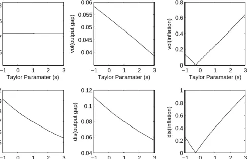
xq= 1 ∆[(δπ−1)κ+ (β−1)δs]sq with ∆ = (δπ−1)γ+δx(1−β) (26) πq=− 1 ∆[δxκ+δsγ]sq (27) We run the model for 500 quarters (32,000 days) with different values forδs as well as 1000 different
realizations of the pseudo random number generator for each δs. Figure 8 illustrates the resulting
volatility and distortion measures.
−1 0 1 2 3 0.0165 0.017 0.0175 0.018 vol(stock price) Taylor Paramater (s) −1 0 1 2 3 0.15 0.16 0.17 0.18 0.19 0.2 dis(stock price) Taylor Paramater (s) −1 0 1 2 3 0.04 0.045 0.05 0.055 0.06 vol(output gap) Taylor Paramater (s) −1 0 1 2 3 0.04 0.06 0.08 0.1 0.12 dis(output gap) Taylor Paramater (s) −1 0 1 2 3 0 0.2 0.4 0.6 0.8 vol(inflation) Taylor Paramater (s) −1 0 1 2 3 0 0.2 0.4 0.6 0.8 1 dis(inflation) Taylor Paramater (s)
Figure 8: The influence of δs on volatility and distortion measures
Both vol(π) and dis(π) become minimal forδs =−0.29. On the one hand, high stock prices have
a direct negative influence on inflation via eq. (11), but on the other, they have an indirect positive influence via eq. (25) ifδs <0. An increase in stock prices leads to a decrease of the interest rate,
which results in an increase of output and inflation via eq. (9) and (10). It is obvious from (27) that both effects cancel out (πq= 0 ∀ q) forδs=−κδγx, which is −0.29 in our calibration.
If the central bank sets δs < −κδγx = −0.29, it increases the volatility of s, x, and π, as well
as the distortion of x and π, compared to δs = −0.29. Only vol(s) does not increase significantly.
This result is perfectly reasonable, since δs < 0 means using monetary policy to additionally blow
up bubbles. As shown above, only a small pro-cyclical reaction to stock market bubbles could be beneficial with respect to vol(π) and dis(π).
Forδs>−κδγx =−0.29, a trade-off exists, which makes an interpretation less clear. The stronger
asset price bubbles are deflated, the lower are vol(x), dis(s), and dis(x), but the higher are vol(π) and dis(π). Monetary policy can therefore very well be used to deflate asset price bubbles and to control the transmission channel through which asset price fluctuations spill over to real markets. This policy, however, comes at the cost of higher volatility and distortion of inflation rates. We are not going into more detail here, but it has become clear so far that, since our model allows for the endogenous emergence of asset price bubbles, it can be used to analyze the question whether the central bank should deflate such bubbles or not. The trade-off suggests that an optimalδs 6= 0
(likelyδs>0) exists, depending on a somehow defined optimality criterion.
4.2 Impact of Transaction Taxes for Real Markets
We now turn to a question, that is recently often debated in the public press: Is it beneficial for the macroeconomy to introduce a tax on financial transactions? Analogous to subsection 4.1, we answer this question by looking at the implications on volatility and distortion ofst,xq, and πq.
Following Tobin (1978), we assume that the tax has to be paid relative to the nominal value traded. Each investment consists of two transactions, so the tax also has to be paid twice. Orders generated inDt−2imply nominal transaction ofDt−2·exp{st−1}int−1 andDt−2·exp{st}int. The
tax rateτ is applied to the absolute nominal value of both transactions (buys and sells are equally taxed). Since tax payments directly reduce the profitability of an investment, eq. (7) changes to:
Ait= (exp{st} −exp{st−1})Dti−2−τ(exp{st}+ exp{st−1})
Dti−2
+dAit−1 (28)
The transaction tax is represented byτ andDti−2
is the absolute value ofDti−2. We run the model
for 500 quarters (32,000 days) with different values for τ as well as 1000 different realizations of the pseudo random number generator for each τ. Figure 9 shows the average of the volatility and
0 0.2 0.4 0.6 0.8 0.005 0.01 0.015 0.02 vol(stock price) Tax Rate 0 0.2 0.4 0.6 0.8 0.05 0.1 0.15 0.2 0.25 dis(stock price) Tax Rate 0 0.2 0.4 0.6 0.8 0.02 0.03 0.04 0.05 0.06 vol(output gap) Tax Rate 0 0.2 0.4 0.6 0.8 0 0.05 0.1 0.15 0.2 dis(output gap) Tax Rate 0 0.2 0.4 0.6 0.8 0.02 0.03 0.04 0.05 0.06 vol(inflation) Tax Rate 0 0.2 0.4 0.6 0.8 0 0.05 0.1 0.15 0.2 dis(inflation) Tax Rate
Figure 9: Impact of Transaction Taxes.
distortion measures with respect to the imposed transaction tax. With higher tax rates, the stock price volatility falls. The distortion of stock prices also falls for small values of the tax, but for tax rates above 0.325% it rises again. The U-shaped distortion function carries over to the real markets, while volatility of those markets differs from that of the financial sector. Instead of falling monotonically, volatility falls for small tax rates (<0.35%) and rises for high values of τ (>0.35%).
Both volatility and distortion curves are equal for x and π. The transmission of stock price disturbances into the real sector is proportional to s for both x and π (see eq. (21)). For our baseline calibration, x and π are even equal in absolute values. Consequently, the measures vol( ) and dis( ) are equal for x and π. These results suggest that transaction taxes could have positive effects for the financial and real markets if they are sufficiently small.37 If they are set too high, they could even be harmful. When taxes become larger than approximately 0.8%, the distorting effect increases strongly.38
Figure 10 compares our results (solid lines) with an isolated ABC financial market model (dashed lines). The volatility of stock prices in both models is identical. The distortion, however, shows 37
This result is known from ABC modeling of financial and foreign exchange markets. See for example Westerhoff (2003), Demary (2008) and references therein.
38
Demary (2008) has suggested to use the kurtosis as a measure for the probability of extreme events when evaluating policy instruments. In our model taxation lowers the kurtosis from 8.1 in case of no tax to 3.2 (3.1) in the case of τ= 0.325% (τ= 0.35%). The introduction of a tax would therefore also be justified by this criterion.
some interesting differences: For small tax rates, our model results in higher distortion. This effect is certainly due to the feedback between the two cross-sectoral channels (described in section 2.3). For tax rates above approximately 0.7%, the results turn reverse, which implies that the macroeconomy executes a stabilizing, mean-reverting pressure on stock prices for higher tax rates.
0 0.2 0.4 0.6 0.8 0.005 0.01 0.015 0.02 vol(stock price) Tax Rate 0 0.2 0.4 0.6 0.8 0 0.1 0.2 0.3 dis(stock price) Tax Rate
Figure 10: Impact of Transaction Taxes. Baseline calibration (solid line) and isolated ABC model (dashed line).
We close this section by expressing some warnings concerning the quantitative results of our analysis. We still have no reliable estimation of the ABC financial market model,39 which makes
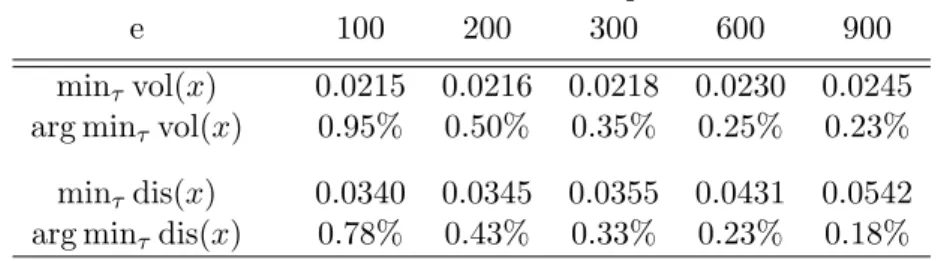
our calibration reasonable, but nonetheless questionable. The optimal tax rates of 0.32% and 0.36% that minimize volatility and distortion in our model could therefore be numerically quite different in reality. To exemplify these concerns, Table 2 presents the minimal volatility and distortion ofx
as well as the corresponding minimizing tax ratesτ for different values of the rationality parameter
e. While the minimal values of vol(x) and dis(x) are rather stable, the minimizing tax rates show considerable differences. They decrease with increasing e. Pellizzari and Westerhoff (2009) have recently shown that the market microstructure, underlying an ABC model, could also have an important influence on the results.
Table 2: Robustness check of the parametere
e 100 200 300 600 900 minτvol(x) 0.0215 0.0216 0.0218 0.0230 0.0245
arg minτvol(x) 0.95% 0.50% 0.35% 0.25% 0.23%
minτdis(x) 0.0340 0.0345 0.0355 0.0431 0.0542
arg minτdis(x) 0.78% 0.43% 0.33% 0.23% 0.18%
39
A first suggestion for the estimation of ABC financial market models (in isolation from real markets) is discussed in Franke and Westerhoff (2009), who argue that the method of simulated moments could be a possible estimation method.
5 Conclusion
We have developed a model that combines agent-based financial market theory with New Keyne-sian macroeconomics. The two employed submodels are simple representatives of their respective disciplin that work basically on their own. They operate on different time scales and use different mechanisms of expectation formation. Interaction between the two models is brought about by two straightforward channels. Our comprehensive model is very stylized and not yet ready for econo-metric analysis. But even with this simplistic methodology, we are able to show that the behavioral structure of financial markets – as formulated in the ABC literature – can have a strong influence on the macroeconomy. First, the emergence of financial bubbles can lead to long-lasting deviations of output and inflation from their steady state. Second, the response of macroeconomic variables to exogenous cost shocks from the real sector itself is also influenced by the animal spirits of the stock market. Impulse response functions become persistent even if the underlying supply shock is non-persistent. This effect is due to the history dependence of the stock market that carries over into the real sector. The on-impact reaction of the real sector to exogenous cost shocks is not influenced by the stock market.
We find that monetary policy can be used to control the spillover of financial market disturbances into the real sector, and that – depending on a somehow defined optimality criterion – an optimal policy reaction to stock prices exists. We also use the model to analyze a question that has recently provoked the public interest, specifically, if the introduction of a transaction tax on financial markets can bring about positive developments for the overall economy. We find that such a tax could generally reduce volatility and distortion of the real and financial market variables, but its size plays a significant role. If it is set too high, the macroeconomy might even be subject to strong distortion. Our model is simple to implement and can be solved algebraically for the real sector. Of course, it can also be used for numerous augmentations: (1) The effects of different cross-sectoral channels (Tobin’s q or stock wealth effect) can be analyzed. (2) The rules that define the behavior of the financial market agents (like the time horizon of investors’ strategies) can be changed. (3) Since the occurrence of bubbles implies large deviations from the fundamental steady state, one might also use a version of the NKM submodel that is not log-linearized. All of these augmentations, however, are unlikely to change our main findings. For example, including a wealth channel instead of a cost channel leaves all qualitative results unchanged. In a recent paper, Demary (2010) augments
the time horizons of the investors and finds that the qualitative results of Westerhoff (2008) are preserved. One can therefore assume that if the investment horizon in our model is augmented in the same way, our results would also persist. Using a numerical solution of a non-linear NKM model instead of an analytical solution of a log-linearized version of the NKM model would clearly also only change results in a quantitative way.
One of the limitations of our model is that the distributional properties of financial markets, like the kurtosis, carry over one for one from quarterly stock prices to output and inflation. These observations suggest that the real economy in our model does not show enough resistance against shocks from the financial markets. Future research should clarify if, for example, the use of sticky wages or hybrid versions of the NKM model (that is characterized by more persistence) yield more realistic results in this respect. One could also criticize our assumptions about the expectation formation of real-market agents about future stock price developments. Instead of forming stationary expectations, these agents might also be influenced by experts who employ the forecasting methods of financial-market agents. For example, one could think of Eq[sq+1] as being the mean of actual
stock prices, an extrapolating and a mean-reverting force. The weights of the latter two can be related to the fractions of chartists and fundamentalists. We do not take financial streams between the real and the financial sector explicitly into account. This simplification should be relaxed in future research. Monetary policy in this paper is modeled in the typical way of macroeconomic analysis by an interest rate rule. But our framework also makes it possible to explicitly model a central bank that buys or sells stock to influence the financial market directly. All these questions and augmentations are left for further research.
References
Aoki, M. and Yoshikawa, H. (2007). Reconstructing Macroeconomics: A Perspective from Statistical Physics and Combinatorial Stochastics Processes, Cambridge University Press.
Bask, M. (2009). Monetary Policy, Stock Price Misalignments and Macroeconomic Instability, Han-ken School of Economics, Working Papers 540.
Becker, M., Friedmann, R. and Kl¨oßner, S. (2007). Intraday Overreaction of Stock Prices, Saarland University, Working Papers.
Bernanke, B. and Gertler, M. (1999). Monetary Policy and Asset Price Volatility,Economic Review
4: 17–51.
Bernanke, B. S., Gertler, M. and Gilchrist, S. (1999). The Financial Accelerator in a Quantitative Business Cycle Framework, In: Handbook of Macroeconomics, Volume I, Edited by J. B. Taylor and M. Woodford, chapter 21, pp. 1341–1393.
Bordo, M. D. and Jeanne, O. (2002). Monetary Policy and Asset Prices: Does ’Benign Neglect’ Make Sense?,International Finance 5: 139–164.
Brock, W. A. and Hommes, C. H. (1998). Heterogeneous Beliefs and Routes to Chaos in a Simple Asset Pricing Model, Journal of Economic Dynamics and Control22: 1235–1274.
Bullard, J. and Schaling, E. (2002). Why the FED Should Ignore the Stock Market,Federal Reserve Bank of St. Louis Review84: 35–41.
Caginalp, G., Porter, D. and Smith, V. (2001). Financial Bubbles: Excess Cash, Momentum and Incomplete Information, Journal of Behavioral Finance 2: 80–99.
Castelnuovo, E. and Nistico, S. (2010). Stock Market Conditions and Monetary Policy in a DSGE Model, Journal of Economic Dynamics and Control 34: 1700–1731.
Colander, D., F¨ollmer, H., Haas, A., Goldberg, M. D., Juselius, K., Kirman, A., Lux, T. and Sloth, B. (2009). The Financial Crisis and the Systemic Failure of Academic Economics,Univ. of Copenhagen Dept. of Economics Discussion Paper No. 09-03.
Colander, D., Howitt, P., Kirman, A., Leijonhufvud, A. and Mehrling, P. (2008). Beyond DSGE Models: Toward an Empirically Based Macroeconomics,American Economic Review98: 236–240. Dawid, H. and Neugart, M. (forthcoming). Agent-Based Models for Economic Policy Design,Eastern
Economic Journal.
De Bondt, W. F. M. and Thaler, R. (1985). Does the Stock Market Overreact?, The Journal of Finance40: 793–805.
De Grauwe, P. (2010). Animal Spirits and Monetary Policy, Economic Theory.
De Grauwe, P. and Grimaldi, M. (2006). Exchange Rate Puzzles: A Tale of Switching Attractors,
European Economic Review 50: 1–33.
Deissenberg, C., van der Hoog, S. and Dawid, H. (2008). EURACE: A Massively Parallel Agent-Based Model of the European Economy, Applied Mathematics and Computation204: 541–552.
Delli Gatti, D., Gaffeo, E. and Gallegati, M. (2010). Complex Agent-Based Macroeconomics: A Manifesto for a New Paradigm, Journal of Economic Interaction and Coordination.
Demary, M. (2008). Who Does a Currency Transaction Tax Harm More: Short-Term Speculators or Long-Term Investors?, Jahrb¨ucher f¨ur National¨okonomie und Statistik (Journal of Economics and Statistics) 228: 228–250.
Demary, M. (2010). Transaction Taxes and Traders with Heterogeneous Investment Horizons in an Agent-Based Financial Market Model,Economics: The Open-Acces, Open-Assessment E-Journal
4.
Fama, E. F. (1965). The Behavior of Stock-Market Prices,The Journal of Business 38: 34–105. Franke, R. and Sacht, S. (2010). Some Observations in the High-Frequency Versions of a Standard
New-Keynesian Model,Christian-Albrechts-Universit¨at Kiel, Economic Working Papers 1. Franke, R. and Westerhoff, F. (2009). Estimation of a Structural Stochastic Volatility Model of
Asset Pricing, Christian-Albrechts-Universit¨at Kiel, Economic Working Papers.
Frankel, J. A. and Froot, K. A. (1987). Using Survey Data to Test Standard Propositions Regarding Exchange Rate Expectations,The American Economic Review 77: 133–153.
Gaffeo, E., Gatti, D. D., Desiderio, S. and Gallegati, M. (2008). Adaptive Microfoundations for Emergent Macroeconomics, Eastern Economic Journal34: 441–463.
Hommes, C. H. (2006). Heterogeneous Agent Models in Economics and Finance, In: Handbook of Computational Economics, Volume 2, Edited by Leigh Tesfatsion ans Kenneth L. Judd., chap-ter 23, pp. 1009–1186.
Hommes, C., Sonnemans, J., Tuinstra, J. and van de Velden, H. (2005). Coordination of Expectations in Asset Pricing Experiments, Review of Financial Studies 18: 955–980.
Howitt, P. (2006). The Microfoundations of the Keynesian Multiplier Process,Journal of Economic Interaction and Coordination1: 33–44.
Ito, T. (1990). Foreign Exchange Rate Expectations: Micro Survey Data,The American Economic Review80: 434–449.
Kirman, A. (1993). Ants, Rationality and Recruitment, The Quarterly Journal of Economics
108: 137–156.
Kirman, A. (2010). The Economic Crisis is a Crisis for Economic Theory, Paper presented at the CESifo Economic Studies Conference on “Whats Wrong with Modern Macroeconomics?”.
Kontonikas, A. and Ioannidis, C. (2005). Should Monetary Policy Respond to Asset Price Misalign-ments?,Economic Modelling22: 1105–1121.
Kontonikas, A. and Montagnoli, A. (2006). Optimal Monetary Policy and Asset Price Misalignments,
Scottish Journal of Political Economy53: 636–654.
Krugman, P. (2009). How Did Economists Get it so Wrong?,New York Times Sept 2.
LeBaron, B. (2006). Agent-Based Computational Finance, In: Handbook of Computational Eco-nomics, Volume 2, Edited by Leigh Tesfatsion ans Kenneth L. Judd., chapter 24, pp. 1187–1233. Lui, Y.-H. and Mole, D. (1998). The Use of Fundamental and Technical Analyses by Foreign Exchange Dealers: Hong Kong Evidence, Journal of International Money and Finance 17: 535– 545.
Lux, T. (2009). Stochastic Behavioral Asset-Pricing Models and the Stylized Facts, In: Handbook of Financial Markets: Dynamics and Evolution. Edited by Thorsten Hens and Klaus R. Schenk-Hopp´e, chapter 3, pp. 161–215.
Lux, T. and Marchesi, M. (2000). Volatility Clustering in Financial Markets: A Micro-Simulation of Interactive Agents, International Journal of Theoratical and Applied Finance 3: 675–702. Lux, T. and Westerhoff, F. (2009). Economics Crisis,Nature Physics5.
Manski, C. and McFadden, D. (1981). Structural Analysis of Discrete Data with Econometric Ap-plications, MIT Press, Cambridge.
Milani, F. (2008). Learning About the Interdependence Between the Macroeconomy and the Stock Market, University of California-Irvine, Department of Economics Working Papers070819. Nam, K., Pyun, C. S. and Avard, S. L. (2001). Asymmetric Reverting Behavior of Short-Horizon
Stock Returns: An Evidence of Stock Market Overreaction, Journal of Banking and Finance
p. 807–824.
Pellizzari, P. and Westerhoff, F. (2009). Some Effects of Transaction Taxes under Differnet Mi-crostructures,Journal of Economic Behavior & Organization72: 850–863.
Ravenna, F. and Walsh, C. E. (2006). Optimal Monetary Policy with the Cost Channel,Journal of Monetary Economics53: 199–216.
Rudebusch, G. D. (2005). Monetary Policy and Asset Price Bubbles, FRBSF Economic Letter. Samanidou, E., Zschischang, E., Stauffer, D. and Lux, T. (2006). Microscopic Models for Financial
Sonnemans, J., Hommes, C., Tuinstra, J. and van de Velden, H. (2004). The Instability of a Heterogeneous Cobweb Economy: A Strategy Experiment on Expectation Formation,Journal of Economic Behavior and Organization54: 453–481.
Taylor, M. P. and Allen, H. (1992). The Use of Technical Analysis in the Foreign Exchange Market,
Journal of International Money and Finance11: 304–314.
Tobin, J. (1978). A Proposal for International Monetary Reform,Eastern Economic Journal4: 153– 159.
Westerhoff, F. (2003). Heterogeneous Traders and the Tobin Tax,Journal of Evolutionary Economics
13: 53–70.
Westerhoff, F. (2008). The Use of Agent-Based Financial Market Models to Test the Effectiveness of Regulatory Policies,Jahrb¨ucher f¨ur National¨okonomie und Statistik (Journal of Economics and Statistics)228: 195–227.
Westerhoff, F. H. and Dieci, R. (2006). The Effectiveness of Keynes-Tobin Transaction Taxes When Heterogeneous Agents Can Trade in Different Markets: A Behavioral Finance Approach,Journal of Economic Dynamics and Control 30: 293–322.