Credit Spreads and the Treasury Zero Coupon Spot Curve

Full text

(1)The University of Reading. THE BUSINESS SCHOOL FOR FINANCIAL MARKETS. Credit Spreads and the Treasury Zero Coupon Spot Curve ISMA Centre Discussion Papers in Finance 2001-06 First version: August 2001 This Version: July 2002. Nicolas Papageorgiou HEC Montreal Frank Skinner ISMA Centre, University of Reading, UK. Copyright 2001 Nicolas Papageorgiou and Frank Skinner. All rights reserved. The University of Reading • ISMA Centre • Whiteknights • PO Box 242 • Reading RG6 6BA • UK Tel: +44 (0)118 931 8239 • Fax: +44 (0)118 931 4741 Email: [email protected] • Web: www.ismacentre.rdg.ac.uk Director: Professor Brian Scott-Quinn, ISMA Chair in Investment Banking The ISMA Centre is supported by the International Securities Market Association.

(2) Abstract This paper examines the relationship between credit spreads on industrial bonds and the underlying Treasury term-structure. Unlike most previous studies, we use zero-coupon spot rates, which eliminate coupon bias, and so allow for a consistent study both within and across the different credit ratings. As far as we are able to determine, we are the first to examine the stability of the relation between credit spreads and the Treasury term structure. We find that the level and the slope of the Treasury term structure are negatively correlated with the spread on corporate bonds. Importantly, the effect of the level and slope of the Treasury yield curve on credit spreads change slowly through time. This is good news for value-at-risk calculations as this suggests that the correlation amongst assets of different credit classes are stable, so use of historic correlations to model spread relations may be valid.. JEL Classification: G21, G24. Key Words: Credit Spread, Coupon Bias, Value at Risk, Correlation. Contacting Authors: Frank S. Skinner (corresponding author), Reader in Finance, ISMA Centre, University of Reading, Whiteknights, Box 242, Reading, RG6 6BA, The United Kingdom. Tel: +44 118 931-6407, Fax: +44 118 93-4741, E-mail: [email protected]. Nicolas Papageorgiou Assistant Professor, HEC Montreal, 3000 Cote St-Catherine, Montreal, PQ, Canada, H3T 2A7. We would like to thank Apostolos Katsaris and Chris Brooks for valuable comments, as well as participants of the International Credit Risk conference in Montreal and FMA Europe conference in Copenhagen. Any errors are our own.. This discussion paper is a preliminary version designed to generate ideas and constructive comment. Please do not circulate or quote without permission. The contents of the paper are presented to the reader in good faith, and neither the author, the ISMA Centre, nor the University, will be held responsible for any losses, financial or otherwise, resulting from actions taken on the basis of its content. Any persons reading the paper are deemed to have accepted this..

(3) ISMA Centre Discussion Papers in Finance DP2001-06. Credit Spreads and the Treasury Zero Coupon Spot Curve The Bank of International Settlement (BIS) requires capital be set aside for credit risk. Therefore, practitioners and academics alike have recently developed credit risk models to quantify credit risk. However, unlike market risks where daily liquid price observations allow a direct calculation of value-at-risk, credit risk is less straightforward to quantify. Models such as JP Morgan’s Creditmetrics seek to construct what they cannot observe: the volatility of value due to credit quality changes. One line of attack is to link movements in the spread between corporate and Treasury yields (the credit spread) to credit events (i.e., credit up and downgrades, defaults). This approach requires a model of the credit spread. Therefore one of the key empirical considerations in modelling credit risk is how to parameterise the relation between Treasury and corporate interest rates. This paper examines the relationship between credit spreads on fixed-income securities that are exposed to default risk and the underlying Treasury term structure. Specifically, we investigate the effects of variations in the level and slope of the Treasury term structure on the credit spreads of investment grade (rated BBB or higher) corporate bonds. This study offers two main contributions to previous work on this topic. Firstly, the study uses zero-coupon spot rates, estimated using the Nelson and Siegel (1987) model. In contrast to most previous work that use yields-to-maturity, the use of zero-coupon spot rates eliminates coupon bias. This clarifies the relationship between Treasury and corporate yield curves and therefore allows for a consistent study both within and across the different credit ratings.1 Secondly, to the best of our knowledge this paper is the first to investigate the stability of the relationships between credit spreads and the Treasury yield curve. The. Copyright 2001 Papageorgiou and Skinner..

(4) ISMA Centre Discussion Papers in Finance DP2001-06. relationships between the variations in the slope and level of the Treasury term structure and the credit spreads are estimated jointly through use of the seemingly unrelated regression errors (SURE) technique thereby correcting for cross-sectional errors and improving the standard errors of the coefficient estimates. We run the regressions for the entire sample period as well as for 51 sub-sample periods. This allows us to investigate both the cross-sectional and time-series properties of the relationships between the factors. We investigate the stability of these relationships by examining the confidence intervals of and test for structural breaks in the response coefficients of the credit spread to changes in the level and slope of the Treasury term structure. We also examine out of sample credit spread prediction errors generated by prior period estimates of the relation between the level and slope of the Treasury term structure and the credit spreads. These prediction errors shed light as to the optimal trade-off between reducing sample error by using a long as possible time series and causing bias by using past outdated data in estimates of the current relationships between the Treasury term structure and the credit spread. The results obtained in this paper are interesting as they provide a comprehensive analysis of the relationship between credit spreads and the underlying Treasury term-structure. Some of our conclusions reinforce previous findings on the topic, whereas others provide new insight into the credit spread / Treasury relationship. We expect that in the absence of call and coupon bias effects, there will be a negative relation between the level and the slope of the Treasury yield curve and the corporate spread. We believe this to be the case because Estrella and Hardouvelis (1991) find that increases in the slope of the term structure foreshadow improvements in real economic activity while Estrella and Mishkin (1998) find that decreases in the. Copyright 2001 Papageorgiou and Skinner.. 2.

(5) ISMA Centre Discussion Papers in Finance DP2001-06. slope of the term structure can indicate an increased likelihood of future recessions. These findings suggest that as the Fed increases short-term rates (and consequently reduces the slope of the term structure), the possibility of future recession increase. We expect that the credit spread would respond to the increased likelihood of future recession. Generally, we find that both the level and the slope are negatively correlated with the spread on corporate bonds, and this relationship is generally significant for all maturities up to 10 years. These results are in agreement with previous studies, with the exception of of Iwanowski and Chandra (1995) and Collin-Duffresne, Goldstein and Martin (2000) who find no significant relation between the slope of the Treasury and the credit spreads. Furthermore, in contrast with Collin-Duffresne, Goldstein, Martin (2000) Duffee (1998), and Longstaff and Schwartz (1995), we do not find that the responsiveness of the credit spreads to changes in the level and slope of the Treasury increases as we move down the credit ratings. Rather, we find statistical evidence suggesting that the responsiveness of the level and slope is constant as we move down the ratings. Furthermore we find a maturity influence where the responsiveness of the credit spread to changes in the level of the term structure at first increases and then decreases with maturity. This differs from previous results presented by Iwanoski and Chandra (1995) who find no maturity influence between Treasury parameters and the credit spreads. Our rolling regressions, structural break tests and the root mean square errors from our out of sample predictions lead us to conclude that the estimated parameters change slowly through time for all maturities. This is of particular interest in regards to value-at-risk calculations, since stable correlation between asset classes implies that historical correlations can be used in a modelling framework. Specifically, we find. Copyright 2001 Papageorgiou and Skinner.. 3.

(6) ISMA Centre Discussion Papers in Finance DP2001-06. that the relation between the level and slope of the Treasury yield curve and the AAA, AA and BBB spread is best estimated using at least four years of monthly data, whereas the same relationships with respect to the A spread is best estimated using two years of monthly data. The paper will be structured in the following manner. Section 1 will provide an overview of what we know about the relationship between credit spreads and the Treasury term structure. Section 2 explains the empirical procedures employed including data selection, term structure estimation and the empirical methodology for investigating the relationship between credit spreads and the Treasury term structure. In section 3 the results will be presented and discussed. Section 4 concludes and summarises.. 1. Credit spreads and the Treasury term structure. In order to parameterise pricing models for credit-sensitive instruments, such as corporate bonds and credit default swaps, it is crucial to understand the joint behaviour of default-free discount rates and the market’s perception of default risk. The relationship between these two variables is, however, not straight forward to assess, and empirical studies have not provided clear results as to the relationship between Treasury yields and credit spreads. There are numerous problems that arise when considering corporate bond data. The most significant problem is that corporate bonds are quoted in terms of their yield to maturity, and most prior empirical studies use this measure rather than zero-coupon spot rates. Yield to maturity calculations are affected by the size of the coupon payment, resulting in what is commonly known as a “coupon-bias”. To appreciate. Copyright 2001 Papageorgiou and Skinner.. 4.

(7) ISMA Centre Discussion Papers in Finance DP2001-06. this, let us consider two corporate bonds in the same rating class, having the same term to maturity, but different coupon payments. The higher-coupon bond will have a lower duration and therefore its yield to maturity will be less sensitive to changes in the underlying default-free rates. Although both bonds are exposed to the same market and credit risk, the responsiveness of their yields to changes in the Treasury termstructure is different. Hence, there is a “coupon-bias” that affects the measure of responsiveness of the bonds to changes in the underlying Treasury term-structure. This bias will affect the results both within a given credit rating, as well across credit ratings. Table 1 shows the average promised coupon as a percentage of face value and the breakdown of the relative coupon sizes for all four credit ratings in our sample, a discussion of our sample selection procedures will follow shortly. As expected, the average coupon size increases as credit quality decreases, since investors demand a higher income from the riskier investment. This result implies that, on average, if two bonds have the same term to maturity, the bond with the lower credit rating will have a smaller duration. This “coupon-bias” will reduce the sensitivity of lower grade bonds to changes in the underlying Treasury term-structure. [Table 1 about here] Another major drawback of many previous studies is that they use bond indexes to calculate credit spreads. These bond indexes are constructed using both callable and non-callable bonds. Yields on callable bonds are, however, affected by the embedded call option, and hence, variations over time of the credit spread will reflect, in part, changes in the call option. Related problems, such as convertibility or other embedded options also complicate the empirical study of the relationship between Treasury yields and corporate credit spreads.. Copyright 2001 Papageorgiou and Skinner.. 5.

(8) ISMA Centre Discussion Papers in Finance DP2001-06. Duffee (1998) looks at the relationship between the Treasury yield to maturity and spreads of corporate less Treasury yield to maturity for both callable and noncallable bonds. He finds that an increase in the 3-month Treasury yield corresponds to a decline in credit spreads. This holds for every combination of maturity and credit rating. The responsiveness of the credit spread to changes in the 3-month Treasury yield increases as credit rating drops. Additionally, the relation between credit spreads and the slope of the Treasury term structure is also found to be negative and increase in magnitude as credit quality drops. Duffee also concludes that the use of yield spreads based on Moody’s yield indexes overestimates the negative relation between the Treasury yields and credit spreads.. He attributes this result to the fact that. Moody’s indexes have historically been constructed primarily with callable bonds. Therefore, results using these indexes are misleading, as the interest rate sensitivity of the bond yield can, in part, be attributed to the change in value of the embedded calloption. More recently, Neal, Rolph and Morris (2000) use a co-integration approach to model the time-series of corporate and government bond rates. They show that corporate rates are co-integrated with government rates and that the relationship is time-dependent. In the short-run, an increase of Treasury rates causes spreads to narrow, but this effect is reversed over the long-run as higher rates cause spreads to widen. The data series they employ for this study includes the monthly averages of the daily yields to maturity for the 10-year constant maturity Treasury Bonds and Moody’s Aaa and Baa seasoned bond indices. The authors select these data series due to their long history (456 months); however, they acknowledge that the bias introduced from the presence of callable bonds is difficult to quantify. In contrast, Kiesel, Perraudin and Taylor (2002), the only prior study that uses zero coupon yields. Copyright 2001 Papageorgiou and Skinner.. 6.

(9) ISMA Centre Discussion Papers in Finance DP2001-06. rather than yield to maturity, shows that that the negative relation between spreads and the level of Treasury interest rates generally remain negative even over long time horizons. Collin-Duffresne, Goldstein, Martin (2000) examine the determinants of credit spread changes by regressing, amongst other variables, changes in the yield on the ten year Benchmark Treasury, and changes in the difference between the 10-year and 2year Benchmark Treasury yield. The credit spreads are calculated using the corporate bond data obtained from Lehman Brothers Fixed Income Database. Consistent with previous findings, they find that an increase in the risk-free rate lowers the credit spread for all bonds. Furthermore, they find that the sensitivity to interest rates increases monotonically across rating groups. They also find that the relation between credit spreads and the slope of the Treasury term-structure is statistically and economically not significant. Again, however, they use yields to maturity rather than zero coupon spot rates and so there results will be affected by the “coupon-bias”. Longstaff and Schwartz (1995) also find that spreads between Moody’s bond yield indexes and Treasury bond yields are strongly negatively correlated. They attribute these results to a presumed negative correlation between the firm’s asset values and default-free interest rates. Irrespective of maturity, the estimated level and slope coefficients are negative and like Duffee (1998) increase in absolute magnitude as the credit quality decreases. Once again, the data includes callable bonds, hence the negative relation could be due to variations in the value of the embedded call options. Iwanoski and Chandra (1995) also examine the relation between yields to maturity of Treasury and non-callable bonds. In contrast to Duffee (1998) and Longstaff and Schwartz (1995) they find only a weak negative relation between the level of Treasury yields and credit spreads, as well as no relation between the. Copyright 2001 Papageorgiou and Skinner.. 7.

(10) ISMA Centre Discussion Papers in Finance DP2001-06. Treasury slope and credit spreads. Furthermore they find no maturity influence between Treasury parameters and the credit spread. Finally, Cornell and Green (1991) examine low-grade bond returns. They find that the returns of low-grade bond are much less responsive to changes in Treasury yield than are high-grade bond yields. They attribute this result to the low duration of low-grade bonds (due to high coupon payments and less restrictive call features). In the case of non-callable low-quality bond yields, however, Duffee (1998) finds that credit spreads are very sensitive to Treasury yields. In summary, there appears to be some disagreement about the relationship between credit spreads and changes in the level and slope of the Treasury yield curve. While most research suggests a negative correlation between Treasury yields and credit spreads, sources disagree about the strength of this relationship and whether the responsiveness of credit spreads to Treasury parameters increase with a deterioration in credit quality. These results however are generally plagued by data problems that include the use of yield to maturity rather than spot rates. Specifically, Neal, Rolph, and Morris (2000), Collin-Duffresne, Goldstein, Martin (2000), Duffee (1998), Longstaff and Schwartz (1995), Iwanoski and Chandra (1995), and Cornell and Green (1991) all use yields to maturity rather than spot rates and thus their results are suspect. In contrast only Kiesel, Perraudin and Taylor (2002) use zero-coupon data, and their results promptly contradict many of the conclusions of Neal, Rolph, and Morris (2000).. Copyright 2001 Papageorgiou and Skinner.. 8.

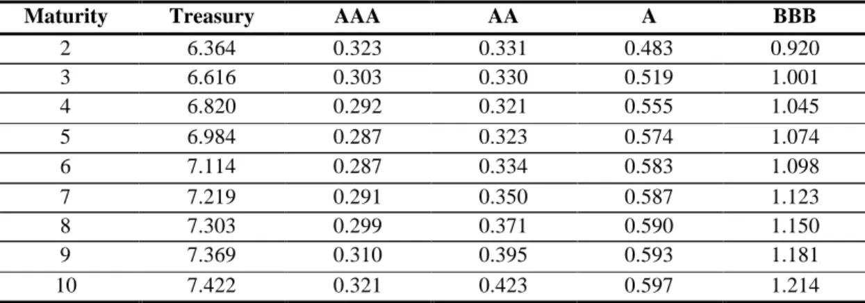
(11) ISMA Centre Discussion Papers in Finance DP2001-06. 2. Empirical Procedures. The first task is to select our data. We employ the University of Houston’s Fixed Income database. This database consists of monthly information on most publicly traded bonds since 1973. The data includes month-end prices (noted as quoted or matrix priced), yields to maturity, time to maturity, coupons, any embedded options, as well as the business sector for each bond (e.g. industrial, financial, utilities). The database also reports the monthly Moody’s and Standard and Poor’s rating for each bond. In this study, a subset of the above database is used. We chose only industrial bonds since we wish to estimate credit risky yield curves that have comparable credit risk all along the yield curve. Hickman (1958) notes that in general we cannot expect that, say an AA industrial bond has the same credit risk as say an AA financial so we at least assure ourselves that our yield curve is constructed from bonds in the same sector category. Additionally there are a sufficiently large number of industrial bonds in all investment rating categories to allow for precise estimation of the corresponding industrial zero-coupon yield curve. We select all bond prices from January 1988 to March 1997, which is the last date in our database. We start our sample in January 1988 for two reasons. First, we wanted to avoid the unusual circumstances surrounding the October 1987 stock market crash. Second, the further back in time one goes, the US bond market becomes less liquid. As the liquidity of the US bond market gradually improved as the US government borrowed more and more in the 80’s, it is not obvious where the start date of our study should be. However, if we include October 1987 we feel we should include many months of prior information to dilute the potential bias this single. Copyright 2001 Papageorgiou and Skinner.. 9.

(12) ISMA Centre Discussion Papers in Finance DP2001-06. observation may create, and then we feel we will be using less liquid information. Hence we choose January 1988 as our start date as we avoid October 1987 and earlier less liquid observations. Next, we eliminated any bonds that had any special features (e.g. put and call options). These embedded features change bond prices and increase price sensitivity with respect to interest rate movements and changes in the business environment. Next, all matrix-priced bonds were eliminated from the sample since Sarig and Warga (1989) and Warga (1991) show that the use of matrix priced information may lead to serious errors. We double-check the remaining sample by eliminating all bonds that are not included in one of the database’s indexes. Since the origin of this data is from Lehman Brothers we believe that bond traders will be more careful in pricing bonds that are included in an index.2 Prior to 1992 the Lehman Brothers corporate bond index only covered investment grade bonds, therefore the analysis in this paper is restricted bonds rated Baa and higher by Moodys (BBB by S&P).3 The selected bonds are divided into four categories: AAA, AA, A, BBB. No distinction is made for bonds with modifiers indicating that a bond is at the upper or lower end of the rating category. Díaz and Skinner (2001) find that shades in credit quality do not significantly affect bond yields for investment grade bonds. Now we estimate zero coupon yield curves for Treasuries, and AAA, AA, A and BBB rated corporates. As noted above, previous empirical studies on corporate bonds have generally defined the corporate spread as the difference between the yield to maturity on a corporate bond and the yield to maturity on a government bond of the same maturity. As this leads to empirical problems we use zero-coupon spot rates as opposed to yields to maturity.. Copyright 2001 Papageorgiou and Skinner.. 10.

(13) ISMA Centre Discussion Papers in Finance DP2001-06. There are two mainstream approaches to estimating the term structure of spot rates. The first is a parsimonious representation defined by an exponential decay term. This approach is developed by Nelson and Siegel (1987) and extended by Svenson (1995). The second approach utilizes a spline representation that can be classified into parametric and non-parametric techniques. McCulloch (1971) introduces the parametric cubic spline, and Fischer, Nychka and Zervos (1995), and Waggoner (1997) develop the non-parametric splines, amongst others.4 In this paper we opt to use parsimonious approaches to estimate both the Treasury and corporate zero-coupon term-structures. We mainly use the Nelson and Siegel (1987) because of its simplicity and proven success. This approach has recently become increasingly popular in empirical literature. Elton et al. (2001) decide to use Nelson and Siegel (1987) in their study finding that their results were almost identical to those obtained using McCulloch (1975). The marked advantages of using Nelson and Siegel (1987), however, is that it imposes a functional form on the term-structure, resulting in a more stable forward (and spot) curve and it requires fewer data points than spline methods. The latter is especially important since certain grades of bonds have relatively few accurately priced bonds in some months. For some months however Nelson and Siegle (1987) proved too inflexible being unable to converge. In these few instances we used Svenson (1995), which is in essence an extension of Nelson and Siegle (1987) that allows for more flexibility in the yield curve shapes. All the parameters for the Nelson and Siegel (1987) and Svenson (1995) models are estimated using Maximum Likelihood, applying the BFGS algorithm to maximise the log likelihood function. We estimate spot rate curves for Treasury bonds as well as for bonds within each of the four corporate rating classes for every month over the period January 1988 through March 1997. We estimate the yield curves up to. Copyright 2001 Papageorgiou and Skinner.. 11.

(14) ISMA Centre Discussion Papers in Finance DP2001-06. ten years maturity because we find like Elton and Green (1998) that beyond ten years the lack of on the run Treasuries created a liquidity problem. In all, 555 maximizations were performed to estimate all the term-structures. The estimation procedure uses the corporate coupon and principle payments as well as the prices of all the bonds within the same rating class on any date, to estimate the full spot yield curve. The number of bonds used to estimate each yield curve is presented in table 2, and range from a minimum of 8 for some AAA term-structures, to 149 for some BBB term-structures. [Table 2 about here] Table 3 contains the average root mean square prediction errors (RMSPE) between theoretical prices computed from the spot rates derived by the Nelson and Siegel procedure and the actual quoted prices. In their paper Elton et al. (2000) ignore AAA rated industrial bonds as they claim that for most of the period studied, the number of these bonds that existed and were dealer quoted was too small to allow for accurate estimation of the term-structure of spot rates. Although the number of outstanding bonds is considerably smaller for the AAA class, the results in table 3 indicate that the RMSPE for the AAA industrial bonds is smaller than for the other credit ratings. This implies that the AAA spot curve is more accurate at pricing the outstanding bonds, and hence we feel this justifies the inclusion of the AAA spot curve in our study. [Table 3 about here] Table 4 reports the average spread from Treasury for AAA, AA, A and BBB bonds in the industrial sector over the entire sample period (111 months). All the data is extracted from the Nelson and Siegel spot curve estimates. Treasuries are reported as annualized spot rates, and corporate spreads are reported as the difference between. Copyright 2001 Papageorgiou and Skinner.. 12.

(15) ISMA Centre Discussion Papers in Finance DP2001-06. the derived corporate spot rates and the derived treasury spot rates. The estimated values seem to be consistent with previous findings as well as with financial theory. The spreads increase in magnitude as we move down the credit ratings, indicating, citerus paribus, a higher default probability for lower grade bonds. Of interest as well is that, except for AAA spreads, the slope of the credit spreads increases with maturity. This term premium increases monotonically as credit-quality decreases. [Table 4 about here] We now select the variables to represent the Treasury term structure. Litterman and Sheinkman (1991) and Chen and Scott (1993) document that the vast majority of variations in the Treasury term structure can be expressed in terms of changes in the level and the slope. Accordingly, we use the one-year Treasury zero coupon yield and the term premium between the ten year Treasury and the one year Treasury zero coupon yield as our measures of the level and slope of the Treasury term structure. To establish the relationship between the corporate yield curve and the Treasury term structure, we regress the first differences in the current level and slope of the Treasury term structure against the changes in the credit spreads. That is,. ∆spread t , j = b0,i + b1,i ∆levelt ,i + b2,i ∆slopet ,i + et ,i. (1). All of the data for the corporate spreads and the Treasury yields is extracted from the estimated zero coupon term structures. Due to the small number of quotes with short terms to maturity, the estimated corporate spot rate curves tend to be relatively unstable at the short end of the curve. For this reason, we only used corporate spot rates that had terms to maturity of at least 12 months. The dependent variable (spread). Copyright 2001 Papageorgiou and Skinner.. 13.

(16) ISMA Centre Discussion Papers in Finance DP2001-06. corresponds to the difference between the corporate spot rate and the Treasury spot rate at the same maturity.. When running (1) we encountered a number of violations of the classical least squares assumptions. The Durbin-Watson statistic clearly indicated the presence of positive first order autocorrelation (as its value was far less than two). We dealt with this autocorrelation by incorporating lagged terms of the variables in equation (1). A Box-Jenkins analysis on the resulting residuals showed little or no residual autocorrelation.. We. then. performed. a. Goldfeld-Quandt. test. to. test. for. heteroscedasticity, and found that the residual variance was related to the level of the one-year Treasury rates. To correct for this, we carried out a weighted least squares estimation on the autocorrelated-adjusted version of (1), with the weights being determined by the level of the Treasury term structure. Finally, we suspect that there is a common influence that jointly affects the Treasury yield curve and the credit spread. If this is the case then even when we correct for autocorrelation and heteroscedasticity, (1) will still violate classical least squares assumptions as it would have a cross-sectional error, i.e., Et[et,i,,et,j] ≠ 0 for credit ratings i and j. This will result in inefficient standard errors.5 To test for this possibility we employed the Breusch and Pagan (1980) test. Their Lagrange multiplier test statistic for crossequation error correlation is. M i −1. λ LM = T ∑∑ rij2 ~ χ M2 ( M −1) / 2 i = 2 j =1. Copyright 2001 Papageorgiou and Skinner.. 14.

(17) ISMA Centre Discussion Papers in Finance DP2001-06. In other words, we find the sum of the squared cross-sectional error correlations amongst the four credit spread regressions and multiply them by the number of observations. This statistic is distributed chi-square with degrees of freedom equivalent to the number of correlations (6) amongst this set of four regressions and we reject the null for large values. Table 5 reveals that we can always reject the null at the one percent significance level, so we estimate (1) using the seemingly unrelated regression error (SURE) technique (see Zellner, 1962) that corrects for cross equation correlated. errors. once. (1). has. been. corrected. for. autocorrelation. and. heteroscedasticity.. [Table 5 about here]. 3. Results Each month, the spread is calculated at quarterly intervals for maturities of one year up to ten years for each credit rating. This results in 37 spreads being calculated each month for every credit rating, and each spread for the AAA, AA, A, and BBB rated bonds are regressed jointly via SURE against changes in the slope and the level of the Treasury. As mentioned above, the level of the Treasury is represented by the 1-year spot rate and the slope by the difference between the ten-year and the 1-year spot rates. We use the one-year Treasury yield to represent the level rather than a shorter term Treasury for the sake of consistency. Since we do not use any corporate data with maturity less than 1 year, we felt it would be sensible to limit our Treasury data to maturities of 12 months or greater.. Copyright 2001 Papageorgiou and Skinner.. 15.

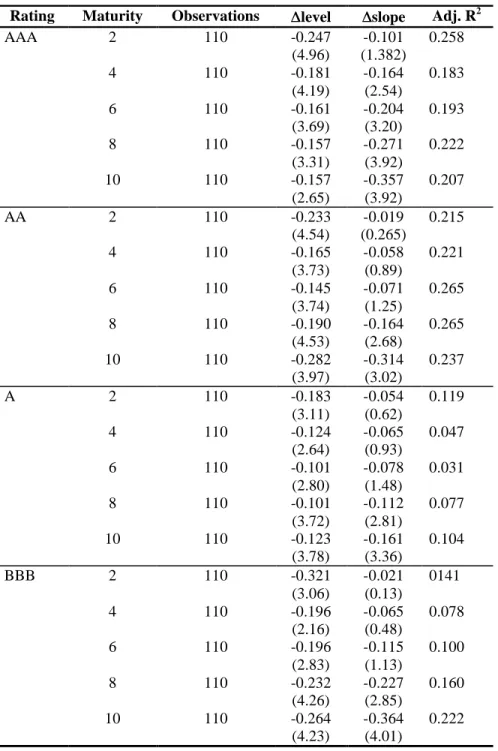
(18) ISMA Centre Discussion Papers in Finance DP2001-06. The results of the regression for the entire sample period are presented in table 6. We show the regression results for maturities of 2, 4, 6, 8 and 10 years and for all four credit ratings.6 The t-statistics are shown in parentheses.. [Table 6 about here]. The estimated coefficient for the change in level is negative for all maturities and all credit ratings. The coefficients range from -0.101 to –0.321 and all are significant at least at the 95% confidence level. The relationship between the changes in the credit spreads and the level of the Treasury term structure does not appear to vary in any regular way with credit quality. In contrast, Duffee (1998), Longstaff and Schwartz (1995), and Collin-Duffresne, Goldstein, Martin (2001) observed a more straightforward relationship. They find that the negative relationship between the changes in the level and the credit spreads strengthens as credit quality falls for all maturities. We attribute the finding of the other authors to their use of yields-tomaturity, and the resulting coupon bias. Table 6 also reports the estimated relation between the slope of the term structure and credit spreads. An increase in the slope corresponds to a decrease in credit spreads, and this relation is statistically significant for all credit ratings at longer maturities, but for bonds rated AA and lower, the slope coefficient is rarely significant for maturities shorter than 6 years. The estimated coefficients range from –0.019 to – 0.364, and there does not appear to be any pattern as we move down the credit ratings. Again these results contrast earlier studies by Duffee (1998) and Longstaff and Schwartz (1995) who find that relationship between the changes in the slope and the credit spreads strengthens as credit quality falls for all maturities7. Collin-Duffresne,. Copyright 2001 Papageorgiou and Skinner.. 16.

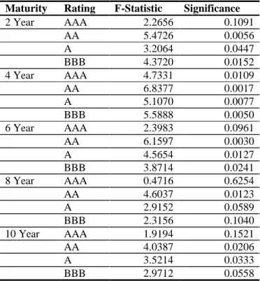
(19) ISMA Centre Discussion Papers in Finance DP2001-06. Goldstein, Martin (2000), and Iwanoski and Chandra (1995) find no significant relation between credit spreads and the slope of the Treasury, independent of rating or maturity. The results obtained by using the SURE regression technique allow us to statistically investigate the stability of the coefficients as we move through the credit ratings for both the level and slope. We use the F-statistic recommended in Judge et al. (1985), pp 475 because it has better finite sample characteristics than the asymptotically valid likelihood ratio test. This F-statistic tests a set of linear restriction of the form Rβ = r , where R and r are known matrices of dimensions (JxK) and (Jx1). The statistic is. λF =. (r − Rβˆ )(RCR') (r − Rβˆ )/ J ~ F( (y − Xβˆ )' (Σ ⊗ I )(y − Xβˆ )/(MT − K ) −1. −1. J , MT − K ). where. [ (. ) ]. C = X ' Σ −1 ⊗ I X. −1. The above F-statistic is calculated for two linear coefficient restrictions on the model. These restrictions are that the four level and slope coefficients are, respectively, equal across credit ratings. Table 7 presents the results of the F-test for maturities of 2, 4, 6, 8, and 10 years for the estimated level and slope coefficients. The null hypothesis, that the level and slope parameters are, respectively, constant across the four credit ratings, cannot be rejected at any significance level for any maturity. This test confirms our earlier suggestion that the credit rating does not affect the magnitude of the response of credit spread movements to shifts in the underlying Treasury term-structure.. Copyright 2001 Papageorgiou and Skinner.. 17.

(20) ISMA Centre Discussion Papers in Finance DP2001-06. [Table 7 about here]. The next step is to look at the stability of the estimated parameters over time. First we conduct a structural break test to determine whether or not the relationships between the level and slope of the term structure and the credit spreads are constant over time. We use dummy variables to split the sample; these dummies take on a value of 1 from February 1988 to August 1993 and a value of 0 from September 1993 to March 1997. We then employ a standard Chow test to measure the significance of the level and slope dummy variables on credit spreads of varying maturities. Table 8 reveals that the dummies are almost always significant, clearly indicating that the relationship between the level and the slope of the Treasury term structure and the credit spreads are not constant.. [Table 8 about here]. This raises a serious issue. Value-at–risk calculations use historic data to estimate the correlations between changes in the term structure and the credit spreads of different credit classes. If these relations are not constant, but change over time, then it is an empirical issue whether current value-at-risk calculations are valid. Specifically, if the relations between the level and slope of the term structure and the structure of credit spreads are unstable, varying radically from period to period, then the use of any amount of historic term structure information to calculate correlations between the Treasury term structure and the structure of credit spreads would be unreliable. However, if the relations between the level and slope of the term structure. Copyright 2001 Papageorgiou and Skinner.. 18.

(21) ISMA Centre Discussion Papers in Finance DP2001-06. and the credit spreads are stable, varying slowly from period to period, then the decision to use historical information to calculate correlation would involve a tradeoff. On the one hand, the use of a longer time-series generally improves the precision of the parameter estimates; on the other hand, if the data is clearly variable across business cycles, incorporating data from too far in the past can result in a bias in the parameter estimates. Having previously shown that estimated slope and level coefficients of the Treasury term-structure are not constant, we now seek to investigate the variability of their relationships with the credit spreads. Are these parameter estimates very volatile? Or do they change slowly over time? We decided to run regression (1) over 51 sub-periods, and investigate the stability of the parameters. Specifically, we run the regression from February 28, 1988 until January 31, 1993, sixty months in all. We then add one month to the data series and re-run the regression once more. We continue to do this for all the remaining months in our sample. The regression is estimated at each of the 37 maturities for each sub-period. In all, the above regression is run for 37 maturities, over 51 sub-samples and for all four credit ratings, a total of 1,887 sets of regressions. These rolling regressions generate 51 estimates of the level and slope coefficients for each credit rating and maturity. We compute the mean and standard deviation of each level and slope coefficient based on a sample size of 51. We then plot the sample mean of the level and slope coefficients along with their respective 95% confidence intervals to generate information about how stable these response coefficients were over the entire sample period. Graphs 1-8 show the rolling regression results for all 51 sub-periods and for all four ratings classes and maturities. The graphs show the 95% confidence intervals for the sub-period level and slope coefficients as well as the mean level and slope. Copyright 2001 Papageorgiou and Skinner.. 19.

(22) ISMA Centre Discussion Papers in Finance DP2001-06. coefficients for all four rating classes. The results are provided quarterly for all maturities between 1 and 10 years. For the AAA rated bonds, the coefficients of the level and the slope are negative for all sub-samples and the 95% confidence intervals are relatively constant at all maturities. For example, at seven years maturity the 95% confidence interval ranges from –0.154 to –0.193 (with a mean of –0.173) for the level estimates and from –0.220 to –0.255 (with a mean of –0.237) for the slope estimates. The results are similar for the AA and A rated industrials. However, the A grade slope coefficient estimates are insignificant for maturities of less than 4.75 years.. [Graphs 1 to 8 about here]. Results for BBB rated bonds are more variable than for the higher credit ratings, particularly on the short end of the maturity spectrum. The slope coefficient is insignificant for terms to maturity less than 5.75 years. Measured at seven years maturity, the 95% confidence interval is -0.193 to -0.331 (mean of –0.262) for the level and –0.127 to –0.180 (mean of –0.153) for the slope. While these confidence intervals are larger than the corresponding ranges for the AAA bonds, the intervals are still modest. These results indicate that the relationship between the level and the slope of the Treasury term structure do not vary much with calendar time. This is good news for value-at–risk calculations since they use historic data to estimate the correlations between the different credit classes and these results suggest that historically estimated correlations, while not constant, are at least stable. Finally, it is evident from graphs 1, 3, 5, and 7 that the responsiveness of the credit spreads to changes in the level of the term structure varies with maturity. For all. Copyright 2001 Papageorgiou and Skinner.. 20.

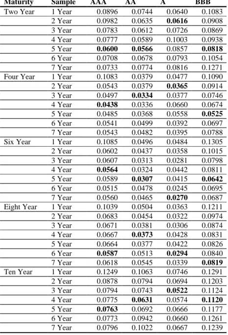
(23) ISMA Centre Discussion Papers in Finance DP2001-06. ratings except AAA, we find that the responsiveness of the credit spread at first increases but then later decreases with maturity. For AAA ratings, the responsiveness increases at a decreasing rate. In contrast, Iwanoski and Chandra (1995) find no significant maturity influence of Treasury parameters on credit spreads. Finding that the relationships between the level and slope of the Treasury term structure and the credit spreads is stable, but not constant, still leaves un-addressed the question of what is the optimal amount of historic data that should be used to reliably estimate these relations. To investigate this question, we run our regressions for one, two, four, six, eight and ten-year credit spreads for all four credit ratings using seven different windows of past data. Specifically we run these regressions based on one, two, three, four, five, six and seven years of monthly data from the immediate past to predict what the credit spread would be next month, say April 1996. We then roll the regression forward one month, and drop the first month in each sample, to predict the credit spread for the subsequent month, May 1996 in our example. We continue to do this for twelve months, until March 1997.8 These spread predictions are based on the historic regression coefficients and the realised value of the level and slope of the Treasury yield curve for the out of sample months. If the relationships between the spread and the Treasury yield curve are very stable, then next month’s level and slope coefficients should not change substantially. Hence, given the current level and slope values, historic level and slope coefficients should closely replicate the actual credit spread. Increasing the sample size tends to lead to more accurate predictions. However, as we stretch our window back in time, the likelihood of using irrelevant data increases which would lead to inaccurate spread predictions. We examine the trade-off between using a longer past time series to improve spread predictions and the use of irrelevant data that increase. Copyright 2001 Papageorgiou and Skinner.. 21.

(24) ISMA Centre Discussion Papers in Finance DP2001-06. prediction error by examining the root mean square prediction error (RMSPE). We expect to see that the RMSPE would at first decrease as we lengthen the past data series, but at some point it will increase as we begin to include past irrelevant data.. [Table 9 about here]. Table 9 reports the result of this experiment for the holdout sample period from April 1996 to March 1997.9 Generally speaking we observe that at first the RMSPE decreases as the estimation period lengthens but then subsequently the RMSPE increases as more and more past data irrelevant to the holdout sample is included in the estimation period. The precise saddle point where RMSPE is smallest does vary depending upon the credit rating and maturity of the predicted spread, but we can make two observations. With only one exception, the AAA, AA and BBB credit spreads all exhibit decreasing RMSPE until at least four years (48 data points) are used to estimate the spread relations. This suggests that one can safely use at least 48 months of past data to estimate the relations between the Treasury yield curve and the AAA, AA and BBB spreads without being unduly concerned with tainting the results with irrelevant data. However, for the A credit spread predictions, the saddle point where the RMSPE is smallest tends to occur much earlier, as early as two years. This suggests that the relation between the level and slope of the Treasury yield curve and the A credit spread is more variable, and only 24 months of data could be used before past data taints the accuracy of the estimated relations. Overall the result of this experiment is encouraging for value-at-risk calculations. Our results suggest that the correlation amongst assets of different credit classes is stable, so use of historic correlations to measure spread relations maybe. Copyright 2001 Papageorgiou and Skinner.. 22.

(25) ISMA Centre Discussion Papers in Finance DP2001-06. valid. In particular we find evidence that supports the use of at least 48 monthly data points to estimate the relationships between the Treasury yield curve and the AAA, AA and BBB credit spread, and at least 24 monthly data points to estimate the relationship between the Treasury yield curve and the A credit spread.. 3.4 Summary and Conclusions. We have examined the relationship between the excess yield on Industrial bonds and the underlying Treasury term-structure. What sets our work apart from previous research on the subject is the quality of the data, as well as the decision to use estimated zero-coupon spot rates rather than yields to maturity. We find that several of our conclusions contradict results from previous papers. We find that an increase in the level and/or slope of the Treasury term-structure results in a decrease in the size of the credit spread. This relation holds for all maturities up to 10 years and for all four credit ratings. In contrast to results presented by Duffee (1998), Longstaff and Schwartz (1995), and Collin-Duffresne, Goldstein, Martin (2000), we do not find that the relationship between the Treasury variables and credit spreads increases in strength as we move down the ratings. To the contrary, we find that the relationship between changes in the credit spread and changes in the level and slope of the Treasury zero yield curve is fairly constant. Using a SURE framework, we cannot reject the null hypothesis that for any given maturity, both the estimated level and slope coefficients are equal across credit ratings. We also find that the responsiveness of the credit spread to changes in the level of the Treasury at first strengthens but later weakens as we move along the yield curve. This also contrasts previous research by. Copyright 2001 Papageorgiou and Skinner.. 23.

(26) ISMA Centre Discussion Papers in Finance DP2001-06. Iwanoski and Chandra (1995) who find that there is no significant relationship between Treasury parameters and the maturity of credit spreads. We also investigated the stability through time of the relationship between changes in the Treasury term structure and changes in the credit spreads. We conclude that both the level and slope coefficients do not vary much over the sample period, and that the estimated coefficients are at all times negative. This is good news for value-at-risk calculations as this suggests that the correlation amongst assets of different credit classes are stable, so use of historic correlations to measure spread relations maybe valid. In particular, we find evidence that supports the use of at least 48 monthly data points to estimate the relationship between the Treasury yield curve and the AAA, AA and BBB credit spread, and at least 24 data points to estimate the relationship between the Treasury yield curve and the A credit spread.. Copyright 2001 Papageorgiou and Skinner.. 24.

(27) ISMA Centre Discussion Papers in Finance DP2001-06. References Breusch, T. S. and A. R. Pagan, 1980, The lagrange multiplier test and its applications to model specification in econometrics, Review of Economic Studies, 47, 239-254. Chen, R., Scott, L. 1993, Maximum likelihood estimation for a multifactor equilibrium model of the term structure of interest rates. Journal of Fixed Income 3, 14-31. Collin-Dufresne, P., Goldstein R, and J.S. Martin, (2001), The determinants of credit spread changes, Journal of Finance, 56 (6): 2177-2207. Cornell, B., Green, K. 1991, The investment performances of low-grade bond funds, Journal of Finance 46, 29-48. Diaz, A., Skinner, F. 2001, Estimating Corporate Yield Curves, Journal of Fixed Income, 11 no.2, 95-103. Duffee, G. 1998, The relationship between treasury yields and corporate bond yield spreads. Journal of Finance 53, 2225-2241. Duffee, G. 1998, Estimating the price of default risk. Review of Financial Studies 12, 197-226. Duffie, D., Singleton, K. 1999, Modelling term structures of defaultable bonds. Review of Financial Studies 12, 687-720. Elton, N., Green, C. 1998, Tax and Liquidity Effects in Pricing Government Bonds. The Journal of Finance 53, 1533-1562. Elton, N, Gruber, M., Agrawal, D., Mann, C. 2001 Explaining the Rate Spread on Corporate Bonds. Journal of Finance 56, 247-277. Fisher, M., Nychka, D., Zervos, D. 1995. Fitting the term structure of interest rates with smoothing splines, Federal Reserve Bank Finance and Economics Discussion Paper 95, 1 January. Green, C., Odegard, A. 1997, Tax effects in relative pricing of U.S. Government bonds. Journal of Finance 52, 609-633. Hickman, W. B. 1958. Corporate bond quality and investor experience. Princeton University Press. Ivanowski, R., Chandra, R. 1995, How do corporate spread curves move over time? Working paper, Salomon Brothers, New York. Judge, G.G., W.E. Griffiths, R. Carter Hill, H. Lutkepohl and T. Lee, 1985, The Theory and Practice of Econometrics, second edition, Wiley, New York.. Copyright 2001 Papageorgiou and Skinner.. 25.

(28) ISMA Centre Discussion Papers in Finance DP2001-06. Kiesel, R., W. Perraudin and A. Taylor, 2002,“Credit and interest rate risk, Risk Management: Value at Risk and Beyond, M.A.H. Dempster (ed.) Cambridge. Litterman, R., Scheinkman, 1991, J. Common factors affecting bond returns. Journal of Fixed Income 1, 54-61. Longstaff, F., Schwartz, E. 1995, A simple approach to valuing risky debt. Journal of Finance 50, 789-821. McCulloch, J. H., 1971, Measuring the term structure of interest rates. Journal of Business 44, 19-31. McCulloch, J. H., 1975, The Tax Adjusted Yield Curve. Journal of Finance 30, 811829. Neal, R., Rolph D., and C. Morris, 2000, Interest rates and credit spread dynamics, Working paper series, Indiana University. Nelson, R., Siegle, F. 1987, Parsimonious modelling of yield curves. Journal of Business 60, 473-489. Sarig, O., Warga, A. 1989, Some empirical estimates of the risk structure of interest rates. Journal of Finance 24, 1351-1360. Svenson, L. 1995, Estimating and interpreting forward interest rates: Sweden 19921994. International Monetary Fund, Working paper, D95-1. Waggoner, D. F. 1997, Spline methods for extracting interest rate curves from coupon bond prices. Federal Reserve Board of Atlanta, Working Paper 97-10. Warga, A. D. 1991, Corporate bond price discrepancies in the dealer and exchange markets. Journal of Fixed Income 1, 7-16. Zellner, Arnold, 1962, An efficient method of estimating seemingly unrelated regressions and tests of aggregation bias," Journal of the American Statistical Association, 1962, v57(298), 348-368.. Copyright 2001 Papageorgiou and Skinner.. 26.

(29) ISMA Centre Discussion Papers in Finance DP2001-06. Table 1. Number of outstanding bonds used in Nelson & Siegel spot curve estimation This table contains the average, minimum and maximum number of bonds used in the estimation of the zero-coupon spot rate curves for the AAA, AA, A, and BBB rated industrial bonds.. AAA AA A BBB. Mean 18.28 67.41 98.55 111.41. St Dev. 7.783 27.98 14.41 46.40. Minimum 8 24 66 37. Maximum 39 128 114 149. Table 2 Coupon size and distribution This table presents a breakdown of the relative coupon size of the industrial bonds for the four credit ratings. The average coupon size and its standard deviation is calculated for each rating class. We also divide the bonds into three groups depending on the coupon size, and show the percentage of outstanding bonds in each coupon range for each credit rating. The coupon ranges are 0% and 6% of face value, 6%-8% of face value, and coupons greater that 8% of face value.. Mean Coupon 7.742 8.057 8.873 9.567. AAA AA A BBB. St. Deviation 0.468 0.518 0.392 0.314. Coupon 0%-6% 8.10% 7.32% 3.83% 0.86%. Coupon 6%-8% 56.41% 35.02% 7.01% 5.19%. Coupon > 8% 35.49% 57.66% 89.16% 93.95%. Table 3 RMSPE. This table contains the average root mean square errors between theoretical prices computed from the spot rates derived by the Nelson and Siegel procedure and the actual quoted prices. For each credit rating class, the root mean square price error is calculated once per period. The number reported is the average of all the root mean squared errors within a class over the period indicated.. Period. AAA. AA. A. BBB. 01/88-03/97 01/88-04/90 05/90-08/92 09/92-12/94 01/95-03/97. 0.3995 0.2451 0.7310 0.3801 0.1982. 0.6299 0.6101 0.7942 0.7007 0.3658. 0.8715 1.2467 1.0164 0.7319 0.4916. 2.2071 2.0367 2.5885 2.3321 1.8648. Copyright 2001 Papageorgiou and Skinner.. 27.

(30) ISMA Centre Discussion Papers in Finance DP2001-06. Table 4. Measured Spread From Treasury This table reports the average spread from Treasury for AAA, AA, A and BBB bonds in the industrial sector. All the data is extracted from the Nelson and Siegel spot curve estimates. Treasuries are reported as annualized spot rates, and corporate rates are reported as the difference between the derived corporate spot rates and the derived treasury spot rates.. Maturity 2 3 4 5 6 7 8 9 10. Treasury 6.364 6.616 6.820 6.984 7.114 7.219 7.303 7.369 7.422. AAA 0.323 0.303 0.292 0.287 0.287 0.291 0.299 0.310 0.321. AA 0.331 0.330 0.321 0.323 0.334 0.350 0.371 0.395 0.423. A 0.483 0.519 0.555 0.574 0.583 0.587 0.590 0.593 0.597. BBB 0.920 1.001 1.045 1.074 1.098 1.123 1.150 1.181 1.214. Table 5 SURE Test In this table we report the results of the Breusch and Pagan (1980) test for seemingly unrelated regression error. The Lagrange multiplier test statistic λLM is the sum of squared correlation between least squared residual errors multiplied by the number of observations, 110 in this instance. The test statistic is distributed chi-squared with 6 degrees of freedom and we reject the null for large values. The critical value at 1% significance is 16.91. Two Year Four Year Six Year Eight Year Ten Year 0.1838 0.4153 0.2114 -0.1427 -0.1509 ρ(AAA,AA) 0.2993 0.3162 0.2299 0.0345 0.1906 ρ(AAA,A) 0.2443 0.2964 0.4159 0.4115 0.3792 ρ(AAA,BBB) 0.1242 0.1974 0.0408 -0.1751 -0.0312 ρ(AA,A) 0.3637 0.2908 0.3891 0.3819 0.2862 ρ(AA,BBB) 0.2697 0.3379 0.3352 0.2862 0.3717 ρ(A,BBB) 44.3836 65.7773 58.9562 49.4298 46.6338 λ LM. Copyright 2001 Papageorgiou and Skinner.. 28.

(31) ISMA Centre Discussion Papers in Finance DP2001-06. Table 6. Results from the seemingly unrelated regression error technique (SURE) In this table we present the results obtained by regressing changes in corporate credit spreads simultaneously for all four credit ratings against changes in the level and slope of Treasury yields over the entire sample period (January 1988 to March 1997). T-statistics are in parenthesis. Rating AAA. AA. A. BBB. Maturity 2. Observations 110. 4. 110. 6. 110. 8. 110. 10. 110. 2. 110. 4. 110. 6. 110. 8. 110. 10. 110. 2. 110. 4. 110. 6. 110. 8. 110. 10. 110. 2. 110. 4. 110. 6. 110. 8. 110. 10. 110. Copyright 2001 Papageorgiou and Skinner.. ∆ level -0.247 (4.96) -0.181 (4.19) -0.161 (3.69) -0.157 (3.31) -0.157 (2.65) -0.233 (4.54) -0.165 (3.73) -0.145 (3.74) -0.190 (4.53) -0.282 (3.97) -0.183 (3.11) -0.124 (2.64) -0.101 (2.80) -0.101 (3.72) -0.123 (3.78) -0.321 (3.06) -0.196 (2.16) -0.196 (2.83) -0.232 (4.26) -0.264 (4.23). 29. ∆slope -0.101 (1.382) -0.164 (2.54) -0.204 (3.20) -0.271 (3.92) -0.357 (3.92) -0.019 (0.265) -0.058 (0.89) -0.071 (1.25) -0.164 (2.68) -0.314 (3.02) -0.054 (0.62) -0.065 (0.93) -0.078 (1.48) -0.112 (2.81) -0.161 (3.36) -0.021 (0.13) -0.065 (0.48) -0.115 (1.13) -0.227 (2.85) -0.364 (4.01). Adj. R2 0.258 0.183 0.193 0.222 0.207 0.215 0.221 0.265 0.265 0.237 0.119 0.047 0.031 0.077 0.104 0141 0.078 0.100 0.160 0.222.

(32) ISMA Centre Discussion Papers in Finance DP2001-06. Table 7 F-test results for parameter restrictions in SURE. This table reports the F-test for equality of the level and slope coefficients across the AAA, AA, A and BBB credit spreads. The critical value at the 5% significance level for degrees of freedom of 3upper and 434 lower is 2.62 and we reject for large values. Maturity. F-test value Level 1.0050 1.0021 1.0055 1.0142 1.0181. 2 4 6 8 10. Slope 1.0022 1.0081 1.0092 1.0113 1.0121. Table 8 Structural break test This table reports the results of a structural break test examining whether the level and slope coefficients of the Treasury term structure are significantly different in determining the AAA, AA, A and BBB credit spread during the first half of the sample period (February, 1998 to August 1993) than in the second half of the sample period (September 1993 to March 1997). The F-statistic has 2 upper and 99 lower degrees of freedom. Maturity 2 Year. 4 Year. 6 Year. 8 Year. 10 Year. Rating AAA AA A BBB AAA AA A BBB AAA AA A BBB AAA AA A BBB AAA AA A BBB. F-Statistic Significance 2.2656 0.1091 5.4726 0.0056 3.2064 0.0447 4.3720 0.0152 4.7331 0.0109 6.8377 0.0017 5.1070 0.0077 5.5888 0.0050 2.3983 0.0961 6.1597 0.0030 4.5654 0.0127 3.8714 0.0241 0.4716 0.6254 4.6037 0.0123 2.9152 0.0589 2.3156 0.1040 1.9194 0.1521 4.0387 0.0206 3.5214 0.0333 2.9712 0.0558. Copyright 2001 Papageorgiou and Skinner.. 30.

(33) ISMA Centre Discussion Papers in Finance DP2001-06. Table 8: Out of sample mean square prediction error. This table reports the out of sample root mean square prediction error (RMSPE) for predicting the credit spread using historic level and slope coefficients based on seven different sample sizes. The lowest RMSPE for each sample is highlighted in bold. Maturity Two Year. Four Year. Six Year. Eight Year. Ten Year. Sample 1 Year 2 Year 3 Year 4 Year 5 Year 6 Year 7 Year 1 Year 2 Year 3 Year 4 Year 5 Year 6 Year 7 Year 1 Year 2 Year 3 Year 4 Year 5 Year 6 Year 7 Year 1 Year 2 Year 3 Year 4 Year 5 Year 6 Year 7 Year 1 Year 2 Year 3 Year 4 Year 5 Year 6 Year 7 Year. AAA AA 0.0896 0.0744 0.0982 0.0635 0.0783 0.0612 0.0777 0.0589 0.0600 0.0566 0.0708 0.0678 0.0733 0.0774 0.1083 0.0379 0.0543 0.0379 0.0497 0.0334 0.0438 0.0336 0.0485 0.0368 0.0541 0.0499 0.0543 0.0482 0.1085 0.0496 0.0602 0.0437 0.0607 0.0313 0.0564 0.0324 0.0589 0.0307 0.0515 0.0478 0.0560 0.0465 0.1039 0.0504 0.0683 0.0454 0.0671 0.0381 0.0667 0.0373 0.0664 0.0377 0.0587 0.0513 0.0618 0.0545 0.1249 0.1063 0.0878 0.0794 0.0794 0.0743 0.0775 0.0631 0.0763 0.0692 0.0773 0.0942 0.0796 0.1022. Copyright 2001 Papageorgiou and Skinner.. 31. A 0.0640 0.0616 0.0726 0.1003 0.0857 0.0793 0.0816 0.0477 0.0365 0.0377 0.0660 0.0558 0.0392 0.0395 0.0484 0.0358 0.0281 0.0442 0.0415 0.0245 0.0270 0.0363 0.0322 0.0306 0.0428 0.0422 0.0294 0.0339 0.0746 0.0694 0.0522 0.0574 0.0666 0.0660 0.0667. BBB 0.1083 0.0908 0.0869 0.0938 0.0818 0.1054 0.1271 0.1090 0.0914 0.0746 0.0674 0.0525 0.0697 0.0788 0.1305 0.1015 0.0798 0.0811 0.0642 0.0695 0.0687 0.1211 0.0974 0.0874 0.0831 0.0826 0.0840 0.0819 0.1291 0.1203 0.1124 0.1120 0.1177 0.1261 0.1239.

(34) ISMA Centre Discussion Papers in Finance DP2001-06. Graph 1 - AAA level coefficients with 95% confidence intervals. 9 25 9. 5 9. 75 10 9.. 8 25 8. 5 8. 75 8.. 7 25 7. 5 7. 75 7.. 6 25 6. 5 6. 75 6.. 5 25 5. 5 5. 75 5.. 4 25 4. 5 4. 75 4.. 3 25 3. 5 3. 75 3.. 2.. 2 25 2. 5 2. 75. 0. -0.05. Values of coefficient. -0.1. -0.15 AAA UPPER LOWER -0.2. -0.25. -0.3. -0.35 Time to maturity. Graph 2 - AAA slope coefficients with 95% confidence levels. 10. 9. 5 9. 75. 9 25 9.. 8. 5 8. 75. 8 25 8.. 7. 5 7. 75. 7 25 7.. 6. 5 6. 75. 6 25 6.. 5. 5 5. 75. 5 25 5.. 4. 5 4. 75. 4 25 4.. 3. 5 3. 75. 3 25 3.. 2. 5 2. 75. 2.. 2 25. 0. -0.05. -0.1. Values of coefficient. -0.15. -0.2 AAA UPPER LOWER. -0.25. -0.3. -0.35. -0.4. -0.45. -0.5 Time to maturity. Copyright 2001 Papageorgiou and Skinner.. 32.

(35) ISMA Centre Discussion Papers in Finance DP2001-06. Graph 3 - AA level coefficients with 95% confidence intervals. 10. 9. 5 9. 75. 9 25 9.. 8. 5 8. 75. 8 25 8.. 7. 5 7. 75. 7 25 7.. 6. 5 6. 75. 6 25 6.. 5. 5 5. 75. 5 25 5.. 4. 5 4. 75. 4 25 4.. 3. 5 3. 75. 3 25 3.. 2. 5 2. 75. 2.. 2 25. 0. -0.05. -0.1. Values of coefficient. -0.15. -0.2. AA UPPER LOWER. -0.25. -0.3. -0.35. -0.4. -0.45 Time to maturity. Graph 4 - AA slope coefficients and 95% confidence interval 0.1. 9 25 9. 5 9. 75 10 9.. 8 25 8. 5 8. 75 8.. 7 25 7. 5 7. 75 7.. 6 25 6. 5 6. 75 6.. 5 25 5. 5 5. 75 5.. 4 25 4. 5 4. 75 4.. 3 25 3. 5 3. 75 3.. 2.. 2 25 2. 5 2. 75. 0. Values of coefficient. -0.1. AA UPPER LOWER. -0.2. -0.3. -0.4. -0.5 Time to maturity. Copyright 2001 Papageorgiou and Skinner.. 33.

(36) ISMA Centre Discussion Papers in Finance DP2001-06. Graph 5 - A level coefficients with 95% confidence level. 10. 9. 5 9. 75. 9 25 9.. 8. 5 8. 75. 8 25 8.. 7. 5 7. 75. 7 25 7.. 6. 5 6. 75. 6 25 6.. 5. 5 5. 75. 5 25 5.. 4. 5 4. 75. 4 25 4.. 3. 5 3. 75. 3 25 3.. 2. 5 2. 75. 2.. 2 25. 0. Value of coefficients. -0.05. -0.1 A UPPER LOWER -0.15. -0.2. -0.25 Time to maturity. Graph 6 - A slope coefficients and 95% conficence interval 0.1. 0.05. Values of coefficient. 9 25 9. 5 9. 75 10 9.. 8 25 8. 5 8. 75 8.. 7 25 7. 5 7. 75 7.. 6 25 6. 5 6. 75 6.. 5 25 5. 5 5. 75 5.. 4 25 4. 5 4. 75 4.. 3 25 3. 5 3. 75 3.. 2.. 2 25 2. 5 2. 75. 0. -0.05 A UPPER LOWER. -0.1. -0.15. -0.2. -0.25. -0.3 Time to maturity. Copyright 2001 Papageorgiou and Skinner.. 34.

(37) ISMA Centre Discussion Papers in Finance DP2001-06. Graph 7 - BBB level coeficients with 95% confidence level. 10. 9. 5 9. 75. 9 25 9.. 8. 5 8. 75. 8 25 8.. 7. 5 7. 75. 7 25 7.. 6. 5 6. 75. 6 25 6.. 5. 5 5. 75. 5 25 5.. 4. 5 4. 75. 4 25 4.. 3. 5 3. 75. 3 25 3.. 2. 5 2. 75. 2.. 2 25. 0. -0.1. Value of coeficients. -0.2. BBB UPPER LOWER. -0.3. -0.4. -0.5. -0.6 Time to maturity. Graph 8 - BBB slope coefficients and 95% confidence interval 0.2. 0.1. Values of the coefficient. 10. 9. 5 9. 75. 9 25 9.. 8. 5 8. 75. 8 25 8.. 7. 5 7. 75. 7 25 7.. 6. 5 6. 75. 6 25 6.. 5. 5 5. 75. 5 25 5.. 4. 5 4. 75. 4 25 4.. 3. 5 3. 75. 3 25 3.. 2. 5 2. 75. 2.. 2 25. 0. -0.1 BBB UPPER LOWER. -0.2. -0.3. -0.4. -0.5. -0.6 Time to maturity. Copyright 2001 Papageorgiou and Skinner.. 35.

(38) ISMA Centre Discussion Papers in Finance DP2001-06. 1. Elton and Gruber et al., (2001) also use spot rates in their study of corporate bond yields. We thank Arthur Warga, who heads up the University of Houston’s fixed income database program, for providing this advice. 3 Rating disagreements between Standard and Poors and Moodys are unusual. The vast majority of rating disagreements between Moodys and Standard and Poors is just one shade of credit rating within the same broad rating category. It is very rare to have disagreements of more than two shades of credit ratings that cross broad rating categories. 4 For a complete overview of the different methods see Green and Odegard (97) or Wagonner (97). 5 See Judge et al (1985), Page 476. 6 Results from the remaining 32 maturities are available from the authors upon request. 7 Duffee also explores the importance of the coupon effect with a simple arithmetic exercise. He suggests that the coupon bias explains half the difference between the estimated slope coefficient between long maturity and short maturity non-AAA bonds. 8 For robustness we also examined another time period, from April 1995 to March 1996. We found almost precisely the same results are reported below. The results of this additional period are available from the authors upon request. 9 To make sure our prediction errors are not biased, consistently over or undershooting the actual spread, we regressed the prediction errors on the change in level and slope of the treasury yield curve. The constant in this regression is a measure of prediction error bias. For both sets of prediction errors, we find that the constant is never significantly different from zero. 2. Copyright 2001 Papageorgiou and Skinner.. 36.

(39)

No results found