Binary decision diagrams and integer programming

Binary Decision Diagrams

and

Integer Programming

Dissertation

zur Erlangung des Grades

des Doktors der Ingenieurwissenschaften

der Naturwissenschaftlich-Technischen Fakultäten

der Universität des Saarlandes

von

Markus Behle

Saarbrücken

2007

Dekan der Naturwissenschaftlich-Technischen Fakultät I: Prof. Dr. Thorsten Herfet

Vorsitzender:

Prof. Dr. Gerhard Weikum, Max-Planck-Institut für Informatik, Saarbrücken Gutachter:

Prof. Dr. Friedrich Eisenbrand, Universität Paderborn

Prof. Dr. Kurt Mehlhorn, Max-Planck-Institut für Informatik, Saarbrücken Beisitzer:

Abstract

In this work we show how Binary Decision Diagrams can be used as a powerful tool for 0/1 Integer Programming and related polyhedral problems.

We develop an output-sensitive algorithm for building a threshold BDD, which repre-sents the feasible 0/1 solutions of a linear constraint, and give a parallel and-operation for threshold BDDs to build the BDD for a 0/1 IP. In addition we construct a 0/1 IP for nding the optimal variable order and computing the variable ordering spectrum of a threshold BDD.

For the investigation of the polyhedral structure of a 0/1 IP we show how BDDs can be applied to count or enumerate all 0/1 vertices of the corresponding 0/1 polytope, enumerate its facets, and nd an optimal solution or count or enumerate all optimal solutions to a linear objective function. Furthermore we developed the freely available tool azove which outperforms existing codes for the enumeration of 0/1 points.

Branch & Cut is today's state-of-the-art method to solve 0/1 IPs. We present a novel approach to generate valid inequalities for 0/1 IPs which is based on BDDs. We im-plemented our BDD based separation routine in a B&C framework. Our computational results show that our approach is well suited to solve small but hard 0/1 IPs.

In dieser Arbeit zeigen wir, wie Binary Decision Diagrams (BDDs) als ein mächtiges Werk-zeug für die 0/1 Ganzzahlige Programmierung (0/1 IP) und zugehörige polyedrische Pro-bleme eingesetzt werden können.

Wir entwickeln einen output-sensitiven Algorithmus zum Bauen eines Threshold BDDs, der die zulässigen 0/1 Lösungen einer linearen Ungleichung darstellt, und beschreiben eine parallele und-Operation für Threshold BDDs, um den BDD für ein 0/1 IP zu bauen. Des Weiteren konstruieren wir ein 0/1 IP zum Finden der optimalen Variablenordnung und zum Berechnen des Variablenordnung Spektrums eines Threshold BDDs.

Zur Untersuchung der polyedrischen Struktur eines 0/1 IPs zeigen wir, wie man mit Hilfe von BDDs alle 0/1 Ecken des dazugehörigen 0/1 Polytops zählt oder enumeriert, seine Facetten enumeriert und zu einer linearen Zielfunktion eine optimale Lösung ndet oder alle optimalen Lösungen zählt oder enumeriert. Darüber hinaus haben wir das frei erhältliche Tool azove entwickelt, welches bestehende Codes für die Enumerierung von 0/1 Punkten geschwindigkeitsmäÿig übertrit.

Branch & Cut ist heutzutage die Methode der Wahl zum Lösen von 0/1 IPs. Wir be-schreiben einen neuartigen Ansatz zur Generierung zulässiger Ungleichungen für 0/1 IPs, der auf BDDs basiert. Unsere BDD-basierte Separierungsroutine haben wir in einem B&C Framework implementiert. Unsere Rechenresultate zeigen, dass unser Ansatz gut zum Lö-sen kleiner und zugleich schwieriger 0/1 IPs geeignet ist.

Acknowledgments

Many people inuenced my work on this thesis. First of all, I thank my advisor Prof. Dr. Fritz Eisenbrand for his advice, encouragement and guidance during the last years. I am thankful for giving me the opportunity to work in his former Discrete Optimization group at the Max-Planck-Institut für Informatik.

I was most fortunate to meet Prof. Dr. Bernd Becker and Ralf Wimmer from the Albert-Ludwigs-Universität Freiburg. They introduced me to the eld of binary decision diagrams and aroused my interests in combining BDDs with integer programming. I want to thank them for the very fruitful collaboration during the last years.

Many thanks go to all people at the Max-Planck-Institut für Informatik for creating such a fruitful and lively environment. In particular, I am grateful to Andreas Karrenbauer for many interesting discussions (not only) concerning research related topics. Furthermore I thank Ernst Althaus and Stefan Funke for their interests in my work and spending time on discussions. In addition, I thank Ernst Althaus for reading parts of the manuscript and his helpful comments.

I am grateful to Prof. Dr. Kurt Mehlhorn for his instant commitment to become a referee of this thesis and for giving me the possibility to nish my work at the MPI.

V

Contents

2.2 Polyhedral problems . . . 7

2.3 Integer Programming . . . 9

3 Binary Decision Diagrams 11 3.1 Weighted threshold BDDs . . . 11 3.1.1 Basic construction . . . 12 3.1.2 Output-sensitive building . . . 14 3.2 Synthesis . . . 17 3.2.1 Sequential and-operation . . . 17 3.2.2 Parallel and-operation . . . 19 3.3 Variable order . . . 20 3.3.1 Pre-construction heuristics . . . 21 3.3.2 Sifting algorithm . . . 22

3.3.3 Size reduction with unused constraints . . . 23

3.3.4 Exact minimization . . . 23

3.3.5 0/1 Integer Programming . . . 25

3.3.6 Variable order spectrum of a threshold function . . . 28

4 Polyhedral problems 29 4.1 Relation between BDD-polytope and ow-polytope . . . 30

4.2 Optimization . . . 33

4.2.1 Ane hull . . . 34

4.2.2 Dimension of a face . . . 35

4.2.3 Polytope inclusion . . . 35

4.2.4 Certicate of correctness for a threshold BDD . . . 35

4.3 0/1 Vertex counting . . . 36

4.4 0/1 Vertex enumeration . . . 37

4.5 azove Computational results . . . 38

4.6 Facet enumeration . . . 42

4.6.1 Projection of extended ow-polytope . . . 43

4.6.2 Gift-wrapping with a BDD . . . 44

4.6.3 Computational results . . . 46

5 Integer Programming 55 5.1 Using BDDs in Branch & Cut . . . 57

5.1.1 Learning . . . 58

5.2 Separation with BDDs . . . 60

5.2.1 Polynomial time solvability of BDD-SEP . . . 60

5.2.2 Separation via solving a Linear Program . . . 61

5.2.3 A cutting plane approach for BDD-SEP . . . 63

5.2.4 Separation via Lagrangean relaxation and the subgradient method . 64 5.3 Heuristic for strengthening inequalities with a BDD . . . 66

5.3.1 Increasing the number of tight vertices . . . 67

5.4 Lifting . . . 68 5.5 Computational results . . . 70 5.5.1 Implementation . . . 71 5.5.2 Benchmark sets . . . 72 5.5.3 Results . . . 72 Summary 79 Zusammenfassung 81 Bibliography 90

1

1 Introduction

1.1 Motivation

Binary Decision Diagrams (BDDs for short) are a datastructure represented by a directed acyclic graph, which aims at a compact and ecient representation of boolean functions. Since their signicant extension in 1986 in the famous paper by Bryant [Bry86] they have received a lot of attention in elds like computational logics and hardware verication. They are used as an industrial strength tool, e.g. in VLSI design [MT98].

One class of BDDs are the so-called threshold BDDs. A threshold BDD represents in a compact way the set of 0/1 vectors which are feasible for a given linear constraint. As there is an obvious relation to the Knapsack problem, and thus to 0/1 integer programming in general, we were attracted by this class of BDDs.

The classical algorithm for building a threshold BDD (see e.g. [Weg00]) is in principle similar to dynamic programming for solving a Knapsack problem (see e.g. [Sch86]). It is a recursive method, which ensures a unique representation of the output by applying certain rules while building the BDD. In particular, isomorphic subgraphs will be detected after being built and then deleted or merged again. This raises our rst question.

Question 1. Can an algorithm be given, which only constructs as many nodes of the graph representation as the threshold BDD consists of?

For many problems in combinatorial optimization there exists a 0/1 integer program-ming (0/1 IP) formulation, i.e. a set of linear constraints together with a linear objective function and a restriction of the variables to 0 or 1. The natural way for building a BDD for such a problem is the following. First build a threshold BDD for each constraint sep-arately, and then use a pairwise and-operator on the set of BDDs in a sequential fashion, until one BDD is left. This way, intermediate BDDs will be constructed which can have a representation size, that is several times larger than that of the nal BDD. This severe problem motivates our next question.

Question 2. Is there a dierent approach for the and-operation, such that the size explo-sion caused by intermediate BDDs can be avoided?

Until now, we looked at the connection between BDDs and 0/1 integer programming only from one point of view. But we are also interested in the opposite direction.

In general, 0/1 integer programming problems are hard to solve although they might have a small representation size. The transformation of such a problem to a BDD shifts these properties, i.e. the representation size possibly gets large while the optimization problem becomes fairly easy to solve. In fact, it reduces to a shortest path problem on a directed acyclic graph which can be solved in linear time in the number of nodes of the graph. This is the main motivation for the investigation of using BDDs in 0/1 integer programming. Apart from optimization, a lot of other tasks can be eciently tackled if the BDD for a 0/1 integer programming problem could be build.

In polyhedral studies of 0/1 polytopes two prominent problems exist. One is the ver-tex enumeration problem: Given a system of inequalities, count or enumerate its feasible 0/1 points. In addition, if a linear objective function is given, compute one optimal solu-tion, or count or enumerate all optimal solutions.

Question 4. How can these tasks be accomplished using BDDs?

Another one is the convex hull problem: Given a set of 0/1 points in dimension d, enumerate the facets of the corresponding polytope.

Question 5. How can BDDs be used for computing the convex hull of 0/1 polytopes? Branch & Cut is an eective method for solving 0/1 IPs. In theory it is also possible to solve such problems by building the according BDD. But the disadvantage of BDDs is, that building the entire BDD is in practice hard. The running time of Branch & Cut depends on many things, among which are the quality of separated cutting planes. A further point of interest is the generation of cutting planes from not only one constraint of the problem formulation but from two or an arbitrary set of constraints. This leads to the nal question.

Question 6. How can we combine advantages of both elds to develop a fast Branch & Cut algorithm using BDDs to generate cutting planes?

1.2 Outline

This thesis focuses on the above questions, mainly from a practical point of view.

We rst review the preliminaries in chapter 2. In particular, we assume that the reader is familiar with combinatorial optimization and integer programming but less familiar with binary decision diagrams.

In chapter 3 we develop a new output-sensitive algorithm for building a threshold BDD which answers question 1. More precisely, our algorithm constructs exactly as many nodes as the nal BDD consists of and does not need any extra memory. Then we are concerned with question 2. We give an and-operation that synthesizes all threshold BDDs in parallel which is also a novelty. Thereby we overcome the problem of explosion in size during computation. Regarding question 3, we develop for the rst time a 0/1 IP, whose optimal solution gives the size and the optimal variable order of a threshold BDD. Usually, the variable ordering spectrum of a BDD is not computable. With the help of this 0/1 IP, we are now able to compute the variable ordering spectrum of a threshold BDD.

1.3. Sources 3

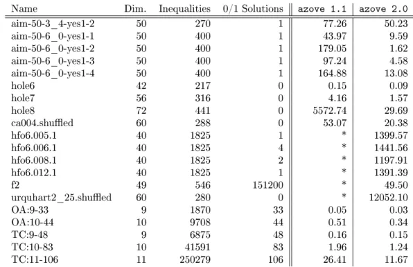
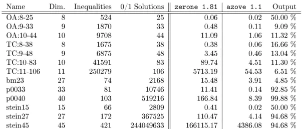
In chapter 4 we are concerned with polyhedral aspects of 0/1 polytopes. We developed a tool called azove1_{, which is capable of vertex counting, enumeration and optimization and}

thus solves the tasks raised by question 4 with the help of BDDs. Computational results show that our tool is currently the fastest available. On some instances, it is several orders of magnitude faster than existing codes. We also investigate the convex hull problem of 0/1 polytopes as raised by question 5. We extend the gift-wrapping algorithm with BDDs to solve the facet enumeration problem. As shown by computational results, our approach can be recommended for 0/1 polytopes whose facets contain few vertices.

Chapter 5 gives a detailed answer to question 6. We apply for the rst time BDDs for separation in a Branch & Cut framework and develop all necessary methods. The computational results which we achieved on MAX-ONES instances and randomly gener-ated 0/1 IPs show, that we developed code which is competitive with state-of-the-art MIP solvers.

1.3 Sources

The material and results in chapters 3 and 4 are from the papers [BE07] and [Beh07a, Beh07b]. The concepts and results in chapter 5 are from the paper [BBEW05].

1_{http://www.mpi-inf.mpg.de/~behle/azove.html, Another Zero One Vertex Enumeration homepage,}

5

2 Preliminaries

In the following we introduce terms and denitions in the way we will use them throughout this work. The sectioning is in dependence on the three main chapters:

3 Binary Decision Diagrams 4 Polyhedral problems 5 Integer Programming

Since the integration of Binary Decision Diagrams into the dierent elds of polyhedral investigation, combinatorial optimization and integer programming is the main aspect of this work, the fundamental terms dened in section 2.1 are essential to know in each chapter.

2.1 Binary Decision Diagrams

This work heavily relies on Binary Decision Diagrams (BDDs for short), a datastructure which represents a set of 0/1 points in a compact way. We provide a denition of BDDs as they are used throughout this work. For further discussions on BDDs we refer the reader to the books [MT98, Weg00].

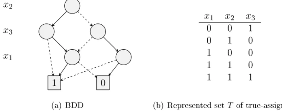
x2 x3 x1 1 0 1 0 (a) BDD x1 x2 x3 0 0 1 0 1 0 1 0 0 1 1 0 1 1 1

(b) Represented setT of true-assignments

Figure 2.1: A simple BDD represented as a directed graph. Edges with parity 0 are dashed. The variable order isx2, x3, x1. The table shows the represented 0/1 points of the set T.

A BDD for a set of dvariables x1, . . . , xd is a directed acyclic graph G= (V, A). An

therootand two nodes with out-degree zero, calledleaf 0resp.leaf 1. There is a labeling

function`:V\ {leaf 0,leaf 1} → {x1, . . . , xd}. All nodes labeled with the variablexi lie on

the same level, which means we have an ordered BDD (OBDD). Thus a level is associated with a variable xi. This relation is given by the variable order, which is a permutation

π:{1, . . . , d} → {x1, . . . , xd}. In this work all BDDs are ordered. For convenience we only

write BDD instead of OBDD.

For the edges there is a parity functionpar : A→ {0,1}. Apart from the leaves all nodes

have exactly two outgoing edges with dierent parity, called the 0-edge resp. the 1-edge according to their parity. Only edges with a direction from top to bottom (concerning the levels) are allowed. A path e1, . . . , ed from the root to one of the leaves represents a

variable assignment in such a way, that the label xi of the head of ej is assigned to the

valuepar(ej). An edge crossing a level with nodes labeledxi is called a long edge. In that

case the assignment for xi is free. If each path from theroot to leaf 1 contains exactlyd

edges the BDD is called complete.

All paths from the root to leaf 1 represent the set T ⊆ {0,1}d _{of true-assignments,}

whereas the paths from theroottoleaf 0represent the setF ⊆ {0,1}d_{of false-assignments.}

We always haveT ∪˙ F ={0,1}d_{. Thus a BDD represents a partition of all 0/1 vertices of}

the unit hypercube in dimensiond.

u v

−→

u

(a) Merging rule

v w

−→

w

(b) Elimination rule

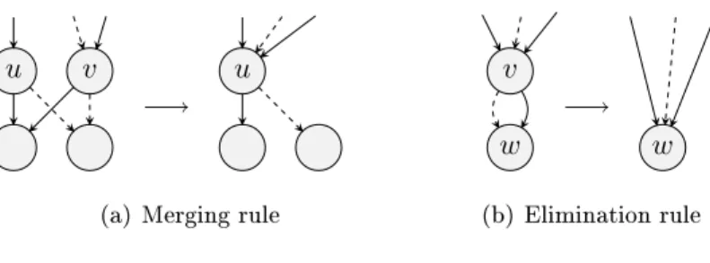
Figure 2.2: The two reduction rules for OBDDs.

Two vertices u, v ∈ V are equivalent, if they have the same label and both of their edges with the same parity point to the same node respectively. A complete and ordered BDD with no equivalent vertices is called a quasi-reduced ordered BDD (QOBDD). A vertexv∈V is redundant, if both outgoing edges point to the same nodew. If an ordered BDD does neither contain equivalent nor redundant vertices it is called reduced ordered BDD (ROBDD). For a xed variable order both QOBDD and ROBDD are canonical representations. In order to achieve such a canonical representation, the following two reduction rules are sucient.

Merging rule: If two verticesu, vare equivalent, then eliminatevand redirect all incoming edges of v tou.

Elimination rule: If vertex v is redundant, then eliminatev and redirect all incoming edges of v to its successorw.

Figure 2.2 illustrates the two reduction rules for OBDDs. Obviously the elimination rule can be applied to a BDD in O(|V|). Bryant's approach [Bry86] to apply the merging rule

2.2. Polyhedral problems 7

needs O(|V|log|V|) time. Sieling and Wegener [SW93] proposed a two phase bucket sort

approach for the merging rule which has linear runtime O(|V|). However it can only be

used after a BDD was built completely.

The size of a BDD is dened as the number of nodes |V|. Let wl be the number of

nodes in level l. The width of a BDD is the maximum of all numbers of nodes in a level w= max{wl |l∈1, . . . , d}. Naturally|V| ≤dwholds. A variable order is called optimal if

it belongs to those variable orders for which the size of the BDD is minimal. The variable ordering spectrum of a linear constraint aTx≤b is the function sp_aT_x≤b: _N→ _N0, where sp_aT_x≤b(k)is the number of variable orderings leading to a BDD of sizekfor the threshold function aTx≤b.

2.2 Polyhedral problems

Next we review some terminology from polyhedral theory that we need in our context in the corresponding chapter 4. Parts of the denitions given in this section are also used in chapter 5 when it comes to polyhedral aspects within integer programming. For a more detailed view on polytopes we refer the reader to the excellent book [Zie95].

First we recall the notion of some standard norms for vectors, i.e. the l1- or 1-norm

kvk₁ :=Pd

i=1|vi|, thel2- or Euclidean norm kvk:=

Pd

i=1vi2

1₂

, and thel∞- or maximum

norm kvk∞:= max1≤i≤d|vi|.

A vector x ∈ _Rd _{is called a linear combination of the vectors x}

1, . . . , xk ∈ Rd, if

x =Pk

i=1λixi for some λ∈Rk. Additionally, if

Pk

i=1λi = 1 holds, x is called an ane

combination. Furthermore if Pk

i=1λi = 1 and λ ≥ 0, x is a convex combination of the

vectors x1, . . . , xk. Given a nonempty set S ⊆ Rd, the set of all vectors which are ane

resp. convex combinations of nitely many vectors ofSare denoted as the ane hullaff(S)

resp. convex hull conv(S) ofS.

A polyhedron P is a set of vectors of the form P ={x∈Rd|Ax≤b} for some matrix

A ∈ _Rm×d _{and some vector b ∈}

Rm. The polyhedron is rational if both A and b can

be chosen to be rational. If P is bounded, then P is called a polytope. The integer hull PI:= conv(P∩Zd) of a polytopeP is the convex hull of the integral vectors in P.

The representation theorem (also called the main theorem) for polytopes states that a polytopeP can be described by two independent characterizations, namely as the convex hull P = conv(S) of a nite point set S (a V-polytope) and as the bounded intersection

of halfspaces P = {x ∈ Rd | Ax ≤ b} (an H-polytope). Both characterizations are in a

certain sense equivalent. This is geometrically clear but nontrivial to prove and we refer the interested reader for the details again to the book [Zie95].

The dimension dim(P) of P is the dimension of its ane hull dim(aff(P)). P is full-dimensional ifdim(P) =d. If P is not full-dimensional then at least one of the describing inequalities ofAx≤bis satised at equality by all points ofP, and thus the interior ofP is empty, i.e.int(P) =∅. Therefore we dene the relative interior ofP as the interior ofP with respect to its embedding into its ane hullaff(P), in whichPis full-dimensional. Note that the maximum number of anely independent points in P isdim(P) + 1and that the

vectorsv0, v1, . . . , vi∈Rdare anely independent i the vectors v1−v0, . . . , vi−v0∈Rd

are linearly independent.

We dene the origin of the vector space Rd as 0 ∈ Rd. If P is full-dimensional and 0∈int(P) holds, the descriptions ofP as aV-polytope and anH-polytope are equivalent

under point/hyperplane duality. For this we need for any setS ⊆_Rd_{the notion of its polar}

S∗ which isS∗:={y∈Rd|yTx≤1for all x∈S}. The extension to that is the so-called

γ-polar of S, which is S_γ∗:={(yT, γ)T ∈_Rd+1_|yT_{x≤γ for allx∈S}.}

A 0/1 polytope is a polytope, which is the convex hull of a set of 0/1 pointsS ⊆ {0,1}d_.

Thus for a 0/1 polytope the notion of its 0/1 points and extremal points resp. vertices is the same since every vertex is a 0/1 point and vice versa. Naturally every 0/1 polytope is contained in the unit hypercube which is dened as {x∈_Rd_|0≤x

i ≤1∀i∈ {1, . . . , d}}.

An inequality cTx ≤ δ with c ∈ _Rd _{and δ ∈}

R is valid for P if it is satised by all

points in P. The faces F of a convex polytope P are ∅, P and the intersection of a supporting hyperplane of P withP itself, i.e. F =P ∩ {x∈_Rd _|cT_{x=δ} withc}T_{x ≤δ}

valid for P. Thus if cTx ≤ δ is valid and δ = max{cTx | x ∈ P}, it denes the face

F ={x∈P |cTx=δ}ofP. The dimension of a faceF of P is the dimension of its ane hulldim(aff(F)). The faceF is a facet ofP, if dim(F) = dim(P)−1. Faces of dimension 0,1,dim(P)−2, anddim(P)−1are called vertices (or extreme points), edges, ridges, and

facets respectively.

A polytope P is called simplicial, if every facet contains exactly dvertices. P is called simple, if every vertex is the intersection of exactly d facets. The input for the facet enumeration problem is called degenerate if there are more than d points which lie on a common hyperplane, and nondegenerate otherwise.

The faces of a polytopeP can be partially ordered by inclusion. Imagine a graph with node layers fromdim(P) down to0, where the nodes in layerirepresent all i-dimensional faces ofP. Thus P is on the top layer and∅on the bottom layer. An edge between a node

in layer i and i+ 1 states that for the corresponding faces Fi ⊃Fi+1 holds. The in this

way constructed graph is a representation of the face lattice of the polytope P.

The facet graph of a polytope P is a graph, whose nodes represent the facets of the polytope P, and with two nodes adjacent by an edge, i the corresponding facets share a common ridge.

Complexity

Dealing with the computational complexity of algorithms for enumeration problems, we consider both the size of the input and the output, since in general the output size might be exponential in the input size.

An algorithm is called output-sensitive if its runtime is bounded in terms of the output size as well as the input size. Implicit in describing an algorithm as output-sensitive is that the dependence on the output size is reasonable, which usually means bounded by a small polynomial (see [Bre96]). Furthermore an enumeration algorithm is called polynomial if its runtime is polynomial in the size of the input and the output for all inputs. A linear algorithm is a polynomial algorithm, whose runtime is linear in the size of the output.

2.3. Integer Programming 9

If the space complexity of an algorithm is polynomial in the input size and not de-pending on the output size, it is called compact. An enumeration problem is strongly

P-enumerable, if there exists a linear and compact algorithm which solves it.

2.3 Integer Programming

We will now give a short introduction to the concepts and terms that we need from the eld of Linear and Integer Programming. This is by far not meant to be a comprehensive survey. More details, further aspects and a deeper insight into this subject can be gained from the book [Sch86].

A Linear Programming (LP) problem asks for an optimal solution of a linear objective function over a polyhedronP. It is usually given in one of its standard forms, i.e.

max cTx s.t. Ax≤b

x∈_Rd

(2.1)

whereA∈Rm×d and b∈Rm dene the polyhedronP and the objective function is given

by c ∈ _Rd_{. There are equivalent forms with Ax = b, Ax ≥ b or bounds l}

i ≤ xi ≤ ui

on the variables xi for i ∈ {1, . . . , d}, but we will mainly use the formulation (2.1). In

addition, the kind of optimization direction can equally be chosen between maximization or minimization. A fundamental result is that Linear Programming is inP (for details see

e.g. [GLSv88]).

In Integer Programming (IP), or more precise Integer Linear Programming, the task is to nd an integer vectorx∈Zd, which is an optimal solution to the problem dened by the

linear objective function and linear constraints given in (2.1). Throughout this work, we will only examine the case of 0/1 Integer Programming (0/1 IP), i.e. we are interested in optimal solutions given by a binary vector x∈ {0,1}d_{. Many combinatorial optimization}

problems are modeled with decision variables and thus can be formulated as 0/1 integer programs. We will use the following standard form for 0/1 IPs

max cTx s.t. Ax≤b

x∈ {0,1}d

(2.2)

where the matrix A and the vectors b and c are rational. 0/1 Integer Programming is

N P-complete. In caseAand bdene the integer hull PI of a 0/1 polytopeP, 0/1 Integer

Programming reduces to Linear Programming. An inequality description of PI however

can be exponential.

A matrix A is called totally unimodular, if each subdeterminant of A is 0, 1 or −1,

so in particular each entry in A is either 0, 1 or −1. There exist a lot of equivalent

characterizations of total unimodularity for a matrixA. If the entries ofA,bandcin (2.2) are integral and Ais totally unimodular, then the linear relaxation 0≤x≤1of (2.2) has

be solved with Linear Programming. In our context we will use the known fact, that the node-edge incidence matrix of a directed graph is totally unimodular.

One of the basic algorithms for solving 0/1 IPs is Branch & Bound. It is an implicit enumeration of the solution space. The problem is decomposed into smaller subproblems by setting up two branches, withxi xed to 0 on one and xed to 1on the other branch.

This recursively leads to a search tree, called the Branch & Bound tree. In addition, for each node a bound on the best solution of its branch is calculated, often via solving the LP relaxation under the given xations. Depending on this bound or the detection of infeasibility, the node will be pruned or the algorithm further branches on it. Among other considerations, maintaining the list of active subproblems and the order of examination of these subproblems are important issues regarding the runtime. Note that a complete enumeration of the solution space is totally impossible for most problems, since there are

2d possibilities.

Another concept to solve a 0/1 IP is the so-called cutting plane algorithm. Here the idea is to solve resp. reoptimize the associated linear programming relaxation. If the solution is fractional, new cutting planes which are valid for the 0/1 IP are found via calling a separation routine. The addition of these cutting planes to the LP relaxation then results in a better approximation of the integer hull. A general method is the application of Chvátal-Gomory cuts which can be generated from an optimal but fractional solution of the LP relaxation. The nature of the applied cutting planes, e.g. whether they are facet-dening for the 0/1 IP, is very import for the running time of this approach. Often the family of valid inequalities generated by a separation routine is enormous. The addition of all these cuts results in big linear programs, which take a long time to solve. Therefore the detection of strong cutting planes is important.

Branch & Cut incorporates ideas from both solution strategies. It is a Branch & Bound algorithm in which cutting planes are generated at the nodes to improve the linear relax-ations. By this, the bound on the best solution of a branch can be tightened, and thus the number of nodes of the Branch & Bound tree can be reduced. In addition, not only cuts are used to improve the performance, but a lot of other techniques like primal heuristics, preprocessing at each node, use of cut pools, and so forth.

Integer programming solvers have become one of the most important industrial strength tools for solving applied optimization problems in the last years. Branch & Cut still is the most successful method for solving 0/1 integer programming problems. It is applied by all competitive commercial codes.

11

3 Binary Decision Diagrams

Binary decision diagrams (or BDDs for short) were rst proposed by Lee in 1959 [Lee59] and further studied by Akers in 1978 [Ake78]. In 1986 Bryant [Bry86]1 _{extended BDDs}

signicantly. He introduced a canonical representation using xed variable ordering, used shared sub-graphs for a compacter representation and presented ecient algorithms for the synthesis of BDDs. After that, BDDs became very popular. Nowadays they are used as an eective datastructure in the area of hardware verication (e.g. VLSI design) and computational logics (e.g. model checking), see e.g. [MT98, Weg00].

In chapters 4 and 5 we extend the usage of BDDs to problems from the elds of poly-hedral investigation, combinatorial optimization and integer programming. In particular we use the fact that 0/1 integer programs are related to knapsack, subset sum and multidi-mensional knapsack problems. Building a BDD for these problems incorporates building a BDD for a linear constraint, a so-called weighted threshold BDD. In section 3.1.2 we present a novel approach for this task which consists of an output-sensitive algorithm for building a threshold BDD. Combining linear constraints relates to an and-operation on threshold BDDs. We provide a parallel and-operation on threshold BDDs in section 3.2.2.

BDDs are represented as a directed acyclic graph. The size of a BDD is the number of nodes of its graph. It heavily depends on the chosen variable order. Bollig and Wegener showed in [BW96] that improving a given variable order is N P-complete. So nding the

optimal variable order is an N P-hard problem. In section 3.3.5 we derive a 0/1 integer

program for nding an optimal variable order of a threshold BDD. With the help of this formulation the computation of the variable order spectrum of a threshold function is possible (see section 3.3.6).

3.1 Weighted threshold BDDs

Denition 3.1. A BDD representing the setT =x∈ {0,1}d_|aT_{x≤b of 0/1 solutions}

to the linear constraint aTx≤b is called a weighted threshold BDD.

The width of a threshold BDD only depends on the weights. For each variable order it is obviously bounded by O(|a1|+. . .+|ad|). Therefore the size of a threshold BDD is

bounded by O(d(|a1|+. . .+|ad|)). If the weights a1, . . . , ad are polynomial bounded in

1_{As of September 2006 this paper is the most cited paper according to CiteSeer.IST, Scientic Literature}

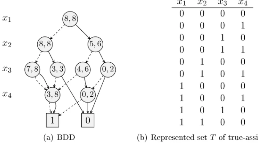
x1 x2 x3 x4 1 0 8,8 8,8 5,6 7,8 3,3 4,6 0,2 3,8 0,2 1 0 (a) BDD x1 x2 x3 x4 0 0 0 0 0 0 0 1 0 0 1 0 0 0 1 1 0 1 0 0 0 1 0 1 1 0 0 0 1 0 0 1 1 0 1 0 1 1 0 0

(b) Represented setT of true-assignments

Figure 3.1: A threshold BDD representing the characteristic function of the linear con-straint2x1+ 5x2+ 4x3+ 3x4≤8. Edges with parity 0 are dashed.

d, the size of the BDD is polynomial bounded in d. For any variable order the size of a threshold BDD is known to be upper bounded by O 2d/2

[HTKY97].

For a long time it was not clear whether all threshold BDDs can be represented in polynomial size with an adaptively chosen variable order. Hosaka et al. [HTKY97] provided an example of an explicitly dened threshold function for which the size of the BDD is exponential for all variable orders. Be keven and d=k2. The linear constraint is dened on the dvariables xij,1 ≤i, j ≤k. Beaij = 2i−1+ 2k+j−1. Then for any variable order

the size of the threshold BDD for the linear constraint P

1≤i,j≤kaijxij ≥k(22k−1)/2 is

lower bounded byΩd2

√

d/2_{. An alternative proof to the one given in [HTKY97] can be}

found in [Weg00].

Denition 3.1 reveals the close relation between building a threshold BDD and solving the knapsack problem

max{cTx|aTx≤b, a∈_Zd, b∈_Z, x∈ {0,1}d}

resp. the subset sum problem

∃x∈ {0,1}d: aTx=b, a∈Zd, b∈Z.

In the following sections we will compare our techniques for building threshold BDDs with the dynamic programming approaches for the knapsack problem presented in [Sch86]. 3.1.1 Basic construction

Consider the function f:{0,1}d _→

Z with f(x) := aTx−b, a ∈ Zd, b ∈ Z. Algorithm

3.1 shows how to build the BDD for the characteristic function of the linear constraint f(x) ≤ 0. It is similar to a dynamic programming approach. We start at the root of

3.1. Weighted threshold BDDs 13

Algorithm 3.1 Build BDD forf(x)≤0

BuildBDD(f) 1: if max(f)≤0then 2: returnleaf 1 3: if min(f)>0 then 4: returnleaf 0 5: if f ∈ComputedTable then 6: return ComputedTable[f] 7: xi = NextVariable(f)

8: BDD low = BuildBDD(f|xi=0) 9: BDD high = BuildBDD(f|_xi=1)

10: BDD result =xi·high + x¯i·low 11: ComputedTable[f] = result

12: return result

the BDD and traverse it in a depth-rst-search manner. For every node we recursively construct its both sons and then build the node itself.

Let a given variable order be xed. Dene a+ := P

ai>0ai and a

− _:= P

ai<0ai. We

set up a table of sized×(a+−a−)in which we save results (step 11) and look up already

computed parts of the BDD in constant time (step 5). To start building the BDD we call BuildBDD(aT_{x−b). First we check for trivial cases (steps 1 and 3). Note that it is}

sucient to compute the global minimum and maximum for f once. These are a− −b resp.a+−b. All other local minima and maxima can be computed in constant time by the recursive calls. After the selection of a variable xi according to the given variable order

(step 7) we build the children of the actual node with restriction of the variable xi to 0

resp. 1 (steps 8 - 9). In step 10 a new node will be inserted on top of both children. This is done by the so-called If-Then-Else-operator (ITE). It is a ternary Boolean function with inputs x,h,lthat computes the function If x, then h, else l

IT E(x, h, l) =x·h+ ¯x·l

The ITE-operator reects Shannon's decomposition rule performed in a node of the BDD: f(x) =xi·f|xi=1+ ¯xi·f|xi=0

The number of variables xed to a value determines the level l on which an operation is performed. In a node on level l be ¯a:=P

xi=1ai the sum of all ai for which xi has been

xed to 1. In step 5 the table will then be accessed at position l×(¯a−a−). Note that

this look-up is not exact, i.e. there exist nodes on a level l which have dierent values ¯a but are equivalent.

Algorithm 3.1 can be adapted to build the BDD for a linear equation f(x) = 0. This

relates to the subset sum problem. The following slight modications have to be ap-plied:

3: replace min(f)>0 with min(f)>0∨max(f)<0

Letkak∞ be the maximum absolute value of all components of the vectora. Then the

following lemma holds.

Lemma 3.1. The runtime and the space complexity for building a BDD for the character-istic function of a linear constraint aTx≤b are both O d2kak∞.

Proof. We set up a table of size d×(a+−a−). The size of the BDD cannot exceed the

table size. With dkak∞≥a+−a− the space complexity holds.

Without the recursive calls in steps 8 and 9 the algorithm has constant runtime. So the runtime only depends on the number of recursive calls. Because of the table the algorithm is never called twice for the same look-upl×(¯a−a−). Thus the runtime is bounded by

the space complexity.

Hence the runtime and space complexity for building a BDD for the characteristic function of a linear constraint are both pseudo-polynomial. In section 4.2 we will see that optimizing according to a linear function cTxcan be done in linear time in the size of the BDD. So the knapsack problem can be solved using a BDD in timeO d2kak∞

.

The same holds for the dynamic programming approach to the knapsack problem. Here a directed graph of size(d+ 1)×(2dkak∞+ 1)is also levelwise allocated (cf. [Sch86]). From

each levellto the next levell+1there are two kinds of edges: edges of type(l, δ)→(l+1, δ)

with costs0and edges of type (l, δ)→(l+ 1, δ+al) with costscl. Any directed path from

(0,0)to (d, b0) withb0 ≤byields a feasible solution. An optimal solution can be computed by nding a shortest path from(0,0)to (d, b0) for someb0 ≤bin linear time in the size of the graph.

The advantage of the BDD approach over the dynamic programming approach however is the use of the ComputedTable. Its leads to a compacter representation of all feasible solutions as isomorphic subgraphs can be detected and reused.

3.1.2 Output-sensitive building

A crucial point of BDD construction algorithms is the in advance detection of equivalent nodes (cf. [MT98]). If equivalent nodes are not fully detected this leads to isomorphic subgraphs. As the representation of QOBDDs and ROBDDs is canonical these isomorphic subgraphs have to be detected and merged at a later stage which is a considerable overhead. In this section we describe a new output-sensitive algorithm that overcomes this drawback. Given a linear constraint aTx ≤ b in dimension d it builds the threshold QOBDD of its characteristic functions. Our detection of equivalent nodes is exact and complete so that only as many nodes will be built as the nal QOBDD consists of. No nodes have to be merged later on.

W.l.o.g. we assume ∀i ∈ {1, . . . , d} ai ≥ 0 (in case ai < 0 substitute xi with1−x¯i).

In order to exclude trivial cases let b ≥0 and Pd

i=1ai > b. For the sake of simplicity be

the given variable order the canonical variable order x1, . . . , xd. We assign weights to the

edges depending on their parity and level. Edges with parity 1 in levellcost al and edges

3.1. Weighted threshold BDDs 15

we introduce for each node, a lower boundlb and an upper bound ub. They describe the interval [lb, ub]. Let cu be the costs of the path from the root to the node u. All nodes

u in level l for which the value b−cu lies in the interval [lbv, ubv] of a node v in level

l are guaranteed to be equivalent with the node v. We call the value b−cu the slack.

Figure 3.1(a) illustrates a threshold QOBDD with the intervals set in each node. Algorithm 3.2 Build QOBDD for the constraintaTx≤b

BuildQOBDD(slack, level) 1: if slack<0 then 2: returnleaf 0 3: if slack≥Pd i=levelai then 4: returnleaf 1

5: if exists nodev in level withlbv ≤slack ≤ubv then 6: returnv

7: build new nodeu in level

8: l= level of node

9: 0-edge son = BuildQOBDD(slack,l+ 1)

10: 1-edge son = BuildQOBDD(slack -al,l+ 1) 11: set lb tomax(lb of 0-edge son,lb of 1-edge son+al) 12: set ub tomin(ub of 0-edge son,ub of 1-edge son+al) 13: returnu

Algorithm 3.2 constructs the QOBDD top-down from a given node in a depth-rst-search manner. We set the bounds for the leaves as follows: lbleaf 0 =−∞,ubleaf 0 =−1,

lbleaf 1 = 0and ubleaf 1=∞. We start at therootwith its slack set tob. While traversing

downwards along an edge in step 9 and 10 we subtract its costs. The sons of a node are built recursively. The slack always reects the value of the right hand side b minus the costscof the path from the rootto the node. In step 5 a node is detected to be equivalent

with an already built nodev in that level if there exists a node v with slack∈[lbv, ubv].

If both sons of a node have been built recursively at step 11 the lower bound is set to the costs of the longest path from the node toleaf 1. In case one of the sons is a long edge

pointing from this level l to leaf 1 the value lbleaf 1 has to be temporarily increased by

Pd

i=l+1ai before. In step 12 the upper bound is set to the costs of the shortest path from

the node toleaf 0minus 1. For this reason the interval [lb, ub]reects the widest possible

interval for equivalent nodes.

Lemma 3.2. The in advance detection of equivalent nodes in algorithm 3.2 is exact and complete.

Proof. Assume to the contrary that in step 7 a new nodeu is built which is equivalent to an existing nodev in the level. Again let cu be the costs of the path from therootto the

nodeu. Because of step 5 we haveb−cu 6∈[lbv, ubv].

Case b−cu < lbv:

In step 11lbv has been computed as the costs of the longest path from the nodevtoleaf 1.

rootto leaf 1using node u with costscu+lbu ≤b, so we have lbu < lbv. As the nodesu

and v are equivalent they are the root of isomorphic subtrees, and thuslbu =lbv holds.

Case b−cu > ubv:

With step 12 ubv is the costs of the shortest path from v to leaf 0 minus 1. Be ubu the

costs of the shortest path fromutoleaf 0minus1. Again the nodesuandvare equivalent so for both the costs we have ubu = ubv. Thus there is a path from root to leaf 0 using

nodeu with costscu+ubu< b which is a contradiction.

Algorithm 3.2 can be modied to work for a given equation, i.e. it can also be used to solve the subset sum problem. The following replacements have to be made:

1: replace slack<0 with slack<0∨slack>Pd

i=levelai 3: replace slack≥Pd

i=levelai with slack= 0∧slack=Pdi=levelai

Be nthe size the threshold QOBDD. We can then formulate the following corollary. Corollary 3.1. The space complexity of algorithm 3.2 is O(nlog(b)).

Proof. Because of lemma 3.2 exactlynnodes are created. The merging rule is not needed. In every node we save two non-negative values which are bounded byb.

In contrast to the basic construction algorithm and the dynamic programming approach discussed in section 3.1.1 the space complexity does not depend on the values of the input but on the input and output size.

Let w be the width of the QOBDD which is naturally bounded by n. The following lemma states that our algorithm is output-sensitive.

Lemma 3.3. The runtime of algorithm 3.2 isO(nlog(w)).

Proof. Searching for an equivalent node in step 5 can be done in time log(w). Without

step 5 and the recursive calls in steps 9 and 10 the algorithm has constant runtime. Thus the runtime only depends on the number of recursive calls. Because of lemma 3.2 there are2n recursive calls.

The size n of the QOBDD is bounded bydw and in addition the width w is bounded bydkak∞. So an upper bound of the runtime isO d2kak∞log(w). In order to construct

a QOBDD with the basic construction algorithm and the dynamic programming approach presented in section 3.1.1, the merging rule needs to be applied afterwards. For each node an equivalent node can be found in timelog(w)with the help of dynamic search trees. Then

with lemma 3.1 the resulting runtime is the same as the upper boundO d2kak∞log(w)

. Sieling and Wegener [SW93] showed how to apply the merging rule to a non-reduced BDD in time linear in the size of the non-reduced BDD. Their approach is based on a two phase bucket sort. However it cannot be used for the in advance detection of equivalent nodes.

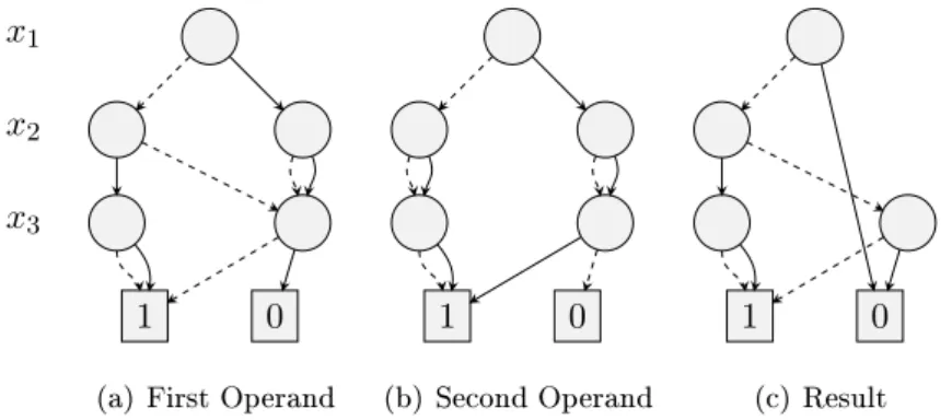
3.2. Synthesis 17 x1 x2 x3 1 0 1 0

(a) First Operand

1 0 1 0 (b) Second Operand 1 0 1 0 (c) Result

Figure 3.2: Conjunction of BDDs: The rst operand is the BDD of the characteristic function of the constraint 2x1−x2+ 3x3 ≤2, the second ofx1−x3 ≤0.

3.2 Synthesis

Now that we know how to build the BDD for a single linear constraint or equation we will tackle 0/1 integer programming problems given in the following form

max{cTx|Ax5b, A∈_Zm×d, b∈_Zm, x∈ {0,1}d}. (3.1) Some or all of themconstraints are allowed to be equations. Although we do not restrictA to be non-negative we consider the input Ax5bas a multidimensional knapsack problem. Our approach consists of two steps. For every of the m constraints construct the BDD of its characteristic function. After that build the conjunction of the BDDs. The nal BDD represents the set of 0/1 solutions to the system Ax5b. Figure 3.2 shows an example of

a conjunction of two BDDs. With the technique described in section 4.2 the optimization problem can then be solved in time linear in the size of the nal BDD.

We describe two ways for the conjunction of BDDs. The classical approach is a pairwise conjunction on the set of BDDs until one nal BDD is left. The size of the intermediate BDDs can be signicantly larger than the size of the nal BDD. Our new method of conjunction avoids this explosion in size by performing an and-operation on all threshold BDDs in parallel.

3.2.1 Sequential and-operation

Let f and g be two boolean functions, e.g. characteristic functions of linear constraints. Be Gf = (Vf, Af) resp. Gg = (Vg, Ag) their graph representations as BDDs. Algorithm

3.3 describes a straight forward recursive approach for the synthesis of two BDDs with the binary operator and (see e.g. [Weg00]).

We start at therootof both BDDsGf andGg. The top-most variable is set to0resp.

1 and for both BDDs the algorithm is called recursively on the two branches. Via the use

of the ComputedTable in steps 5 and 11 we push the detection and reusage of isomorphic subgraphs.

Algorithm 3.3 Conjunction of the two BDDs Gf and Gg

andBDDs(Gf,Gg)

1: if Gf = leaf 1∧Gg= leaf 1 then 2: returnleaf 1

3: if Gf = leaf 0∨Gg= leaf 0 then 4: returnleaf 0

5: if (Gf, Gg)∈ ComputedTable then 6: return ComputedTable[(Gf, Gg)] 7: xi = NextVariable((Gf, Gg))

8: BDD low = andBDDs(Gf|xi=0,Gg|xi=0) 9: BDD high = andBDDs(Gf|xi=1,Gg|xi=1) 10: BDD result =xi·high + x¯i·low

11: ComputedTable[(Gf, Gg)] = result 12: return result

Lemma 3.4. The binary synthesis of the two BDDs Gf and Gg with the operator and is

possible in time and space O(|Vf||Vg|).

Proof. Since all steps can be performed in constant runtime only the number of recursive calls is important. The number of reachable nodes in Gf ×Gg determines the maximal

size of the computed table and thus the runtime.

In practice the typical performance is closer to the size of the resulting BDD which is often smaller than |Vf||Vg|. Note that algorithm 3.3 can be used for the synthesis of any

kind of BDDs, not only threshold BDDs.

Now we return to the 0/1 integer programming problem (3.1). Assume that for all of the m constraints a threshold BDD has been built. Again we point out that these m constraints can be equations or inequalities. Let set B consist of these m BDDs. We iteratively pick two BDDs from B, compute their conjunction with algorithm 3.3 and put the result back in B until one BDD is left in B. This nal BDD then represents the characteristic function of the systemAx5b. LetAmax be the maximum absolute value of

all components of the matrixA. Then lemma 3.1 and the sequential use of the lemma 3.4 leads to the following corollary.

Corollary 3.2. The runtime and the space complexity for the conjunction of m threshold BDDs dened by the system of linear inequalities Ax5b are both O (d2Amax)m

.

Given a BDD and a linear objective function, optimization can be performed in time linear in the size of the BDD, see section 4.2. So for any xed number of constraints m the 0/1 integer programming problem (3.1) can be solved in pseudo-polynomial time.

It is known that the integer programming problem withAx=b,x≥0 andx∈Zdcan

be solved in pseudo-polynomial time for any xed number of constraints [Pap81]. IfAx=b has a solutionx≥0it also has one with entries bounded bydM withM = (mAmax)2m+1.

3.2. Synthesis 19

The order of the BDDs chosen from B for the pairwise conjunction decides on the size of the intermediate BDDs. In order to keep the size of each conjunction small it is advisable to choose the two smallest BDDs. Even though the size of the nal BDD is small an explosion in the sizes of the intermediate BDDs may not be prevented in general. 3.2.2 Parallel and-operation

Our goal is to circumvent the explosion in size while building the nal BDD. Therefore we abstain from using intermediate BDDs by constructing the nal BDD right from the beginning. Given a set of inequalities Ax 5 b, A ∈ Zm×d, b ∈ Zm, we want to build

the ROBDD representing all 0/1 points satisfying the system. For each of the m linear constraints let the threshold QOBDDs be built with the method described in section 3.1.2. Then we build the nal ROBDD by performing an and-operation on all threshold QOBDDs in parallel. The space consumption for saving the nodes is exactly the number of nodes that the nal ROBDD consists of plus d temporary nodes. Algorithm 3.4 describes our parallel and-synthesis ofm QOBDDs.

Algorithm 3.4 Parallel conjunction of the QOBDDsG1, . . . , Gm

parallelAndBDDs(G1, . . . , Gm) 1: if ∀i∈ {1, . . . , m}: Gi = leaf 1then 2: returnleaf 1

3: if ∃i∈ {1, . . . , m}: Gi = leaf 0then 4: returnleaf 0

5: if signature(G1, . . . , Gm)∈ ComputedTable then 6: return ComputedTable[signature(G1, . . . , Gm)] 7: xi = NextVariable(G1, . . . , Gm)

8: 0-edge son = parallelAndBDDs(G1|xi=0, . . . , Gm|xi=0) 9: 1-edge son = parallelAndBDDs(G1|xi=1, . . . , Gm|xi=1) 10: if 0-edge son = 1-edge son then

11: return 0-edge son

12: if ∃node v in this level with same sons then

13: returnv

14: build nodeu with 0-edge and 1-edge son

15: ComputedTable[signature(G1, . . . , Gm)] =u 16: returnu

We start at therootof all QOBDDs and construct the ROBDD from its root top-down

in a depth-rst-search manner. In steps 1 and 3 we check in parallel for trivial cases. Next we generate a signature for this temporary node of the ROBDD in step 5. This signature is a 1 +m dimensional vector consisting of the current level and the upper bounds saved in all current nodes of the QOBDDs. If there already exists a node in the ROBDD with the same signature we have found an equivalent node and return it. Otherwise we start building both sons recursively from this temporary node in steps 8 and 9. From all starting nodes in the QOBDDs we traverse the edges with the same parity in parallel.

When both sons of a temporary node in the ROBDD were built we check its redundancy in step 10. In step 12 we search for an already existing node in the current level which is equivalent to the temporary node. If neither is the case we build this node in the ROBDD and save its signature.

Be n the size of the nal ROBDD. The following lemma states that algorithm 3.4 prevents an explosion in the size needed for the construction.

Lemma 3.5. Algorithm 3.4 needs n + d nodes for the construction of the ROBDD plus additional space for the ComputedTable.

Proof. For every of the d levels a temporary node is needed. In a level a node of the ROBDD will only be built if it is not equivalent to an existing node. The size of the ComputedTable for saving the signatures is bounded by the number of reachable nodes in G1×. . .×Gm.

Now be w the width of the nal ROBDD. Assume that enough space is available for storing the complete ComputedTable with size Qm

i=1|Gi|. Then we have the following

lemma.

Lemma 3.6. The runtime of algorithm 3.4 isO((m+ log(w))Qm

i=1|Gi|).

Proof. For the checks in steps 1 and 3 and the computation of the signature in step 5 all QOBDDs have to be accessed. Hence the runtimes of these operations are O(m).

The look-up and the insert in the ComputedTable in steps 5 and 15 and the check for redundancy in step 10 are possible in constant time. Searching an equivalent node in step 12 can be accomplished inO(log(w)). The main factor for the runtime is the number of

recursive calls. These are bounded by the maximum possible size of the ComputedTable which is Qm

i=1|Gi|.

In practice the main problem of the parallel and-operation is the low hitrate of the Com-putedTable. This is because equivalent nodes of the ROBDD can have dierent signatures and thus are not detected in step 5. In addition the space consumption for the Comput-edTable is enormous and one is usually interested in restricting it. The space available for saving the signatures in the ComputedTable can be changed dynamically. This controls the runtime in the following way. The more space is granted for the ComputedTable the more likely equivalent node will be detected in advance which decreases the runtime. Note that because of the check for equivalence in step 12 the correctness of the algorithm does not depend on the use of the ComputedTable. If the use of the ComputedTable is little the algorithm naturally tends to exponential runtime.

Nevertheless the advantage of algorithm 3.4 in comparison to algorithm 3.3 is that the size of the nal ROBDD is an exact limit on the space needed for the construction.

3.3 Variable order

It is well-known that the variable order used in a BDD has a great inuence on its size (cf. [Weg00]). For BDDs representing a threshold function the assignment of variables with

3.3. Variable order 21

larger weights has a high impact on the weighted sum of the input. Therefore it is likely that the descending order of the absolute values of the weights yields a variable order for which the size of the threshold BDD is small. Hosaka et al. [HTKY97] provided an example which is contrary to this intuition. Given a positive even numberdand the linear constraint Pd/2

i=12i−1xi+Pdi=d/2+1(2d/2−2d−i)xi ≥2d/2d/4. The size of the corresponding threshold

BDD is bounded below by d/2 d/4

if the variables are ordered according to descending weights xdxd−1. . . x1, whereas for the variable orderx1xdx2xd−1. . . xd/2xd/2+1the upper bound for

the size isO d2.

Nevertheless in practice the total order of weights is a good indicator for choosing a variable order which might lead to a small size of the BDD. Finding a variable order for which the size of a BDD is minimal is a dicult task. Bollig and Wegener [BW96] showed that improving a given variable order of a general BDD is N P-complete. Thus it is a N P-hard problem to nd an optimal variable order. We derive a 0/1 integer program in

section 3.3.5 whose optimal solution gives the minimal size and an optimal variable order for the threshold BDD of a given linear constraint. In section 3.3.6 this formulation is the basis for the computation of the variable order spectrum of a threshold function.

3.3.1 Pre-construction heuristics

Before we start to build the BDD for a set of constraints Ax 5 b we have to choose an initial variable order. This variable order should preferably lead to a BDD with small size. Experiments have shown that heuristics which do not take the structure of the problem into account tend to produce bad variable orders. We developed two heuristics which consider all constraints Ax5b and compute an appropriate initial variable order. Both consist of three steps. First the constraint setAx5bis partitioned into subsets, the so-called blocks. Then for every block a partial variable order is computed. In the last step these partial variable orders are merged into one global variable order. The two heuristics only dier in the way they divide up the set of constraints into blocks.

For the partitioning of the constraints in the rst step we adapt an algorithm which is designed for partitioning the outputs of circuits [HKB04]. Dene the support of a constraint over the variables x1, . . . , xd as the set of variable indices with nonzero coecients, i.e.

supp(aTx ≤ b) := {i∈ {1, . . . , d} |ai 6= 0}. We sort the constraints in decreasing order

of the size of their support. Now start with a new initially empty block. The constraint with the largest support is deleted from the set of constraints and inserted into the new block. This constraint is called the leader of the block. Then all constraints satisfying a certain criterion are moved to the new block. If there are still constraints remaining we construct a new empty block and iterate the procedure until the set of constraints becomes empty. We use two dierent criteria to determine if a constraint belongs to a block, the Word-oriented Output Grouping and the Bit-oriented Output Grouping:

• WOG: Add a constraint if its support is a subset of the support of the leader. • BOG: Add a constraint if its support is a subset of the supports of all constraints

The idea behind both criteria is to group constraints with similar support as they can share the same structure in the BDD. In [HKB04] it is shown that the WOG heuristic tends to generate less blocks than the BOG heuristic.

Once the blocks were built we use a simple heuristic to compute the partial orders for every block. BeA0x5b0 the set of constraints belonging to a block. For every variablexj

in the block we compute the sum of the absolute values of its coecients wj :=

Pm0 i=1|a

0 ij|

and then sort the variables in decreasing order of theirwj value. This partial variable order

reects that variables with larger coecients likely have a higher impact on the structure of the BDD.

Before we construct the global variable order with the help of the partial variable orders we sort the blocks increasingly by the number of variables contained in them. Then we merge the partial variable orders given by the blocks using a technique called interleaving [FOH93]. Given the global variable order and a block with a partial variable order that we want to merge into it. The interleaving algorithm works in the following way. Check every variablexi in the block in the order given by the partial variable order if it is already

contained in the global variable order. If this is the case proceed to the next variable. Otherwise determine its predecessor xj in the partial variable order and insert xi in the

global variable order behind xj. If xi is the topmost variable of the partial variable order

insert it at the top of the global variable order. Thus the interleaving algorithm preserves the structures of the partial variable orders within the global variable order.

3.3.2 Sifting algorithm

In section 3.2.1 we have observed that during the sequential conjunction of BDDs the size of the intermediate BDDs might grow drastically. It is desirable to reduce the size after a certain limit in size is exceeded. Among the methods to improve the variable order by dynamic reordering (cf. [MT98] for an overview) is the well-known sifting algorithm by Rudell [Rud93]. It can be applied after the construction of a general BDD. We will describe the algorithm in the following.

The sifting algorithm is based on the swap-operator which locally exchanges the order of two successive variables. W.l.o.g. be the variable order canonical x1, . . . , xd. Then the

swap operation on the variable xi exchanges xi with its successor xi+1 in the BDD. This

local reordering only aects the levelsiand i+ 1 and the runtime is linear in the number

of nodes of both levels. An ecient implementation of the swap-operator is described in [MT98].

Next we use the swap operation to nd a locally optimum position for a variable xi

assuming that all other variables remain xed. Start at the current level of xi and move

xi down by swapping it with its successor until xi reaches the last leveld. Then use the

swap-operator to move xi upwards until it is at the root. During the down and upward

movements of xi we nd the positionj with the smallest size of the BDD. At last we use

the swap-operator to movexi from the root to that levelj. In order to reduce the number

of swap operations the rst moving direction can be chosen adaptively, i.e. if xi is closer

to the root it will rst be moved upwards and afterwards down to the last level.

3.3. Variable order 23

based on the number of nodes in the current level of the variable. According to this sorting then nd for each variable a locally optimum position. We start with the variable which occurs most as a label of a node since it possesses the largest optimization potential.

Be wthe width of the BDD. The algorithm needs O d2

swap-operations which have a complexity of O(w)each. As the runtime of the sorting is dominated by the number of

swap-operations the runtime of the sifting algorithm isO d2w. 3.3.3 Size reduction with unused constraints

Our aim is to build the BDD for a set of constraints Ax≤b. Now assume that we have only achieved to build the BDD for a subset A0x ≤ b0 of the constraints Ax ≤ b so far. Possible reasons are that we did not nish the sequential conjunction (see section 3.2.1) yet or that we could not nish it because the memory or time consumption is too high. So there are some constraints left in the set Ax≤b which are not included in A0x≤b0 and thus have not been used for building the current BDD. In the following we show how to apply these unused constraints to decrease the size of the BDD.

Let aTx ≤ b be such an unused constraint. For each edge in the BDD we set the following weights (compare (4.3) in section 4.2):

w(e) =

(

ai if par(e) = 1 and`(head(e)) =xi

0 if par(e) = 0 otherwise

For all nodes v ∈ V of the BDD we compute the length l↓(v) of the shortest path

starting from theroot to it. Next we compute the length l↑(v) of the shortest path from

leaf 1 upwards to all nodes v. Then the value l(v) := l↓(v) +l↑(v) determines the length

of the shortest path from the rootto leaf 1crossing nodev. We observe the following:

• If there exists a nodev with l(v) > b all paths crossing this node represent vectors

ˆ

x∈ {0,1}d _withaT_{x > bˆ . =⇒Delete v and redirect all incoming edges to leaf 0.}

For all edges e ∈ A we can determine the length of the shortest path from the root to leaf 1 using edgee asl0(e) :=l↓(head(e)) +w(e) +l↑(tail(e)). Then the extension of our

observation reads as follows:

• If there exists an edge e with l0(e) > b all paths using this edge represent vectors

ˆ

x∈ {0,1}d _withaT_{x > b.ˆ =⇒Redirect the tail of eto leaf 0.}

As the graph representation of the BDD is acyclic the shortest path computations run in linear time in the size of the BDD.

These reductions can be applied to the BDD for all unused constraints in Ax ≤ b. Depending on the structure of aTx≤b andA0x≤b0 the size of the BDD reduces consid-erably.

3.3.4 Exact minimization

In the following we give a survey of the development of techniques for the exact minimiza-tion of BDDs. All algorithms aim at computing a variable order for which the size of the

BDD is minimal. They can be applied to all types of BDDs. Nearly all of them are based on the classic method by Friedman and Supowit [FS90] and continuously improve on each other.

Friedman and Supowit [FS90] gave the rst algorithm to nd an optimal variable order. Instead of trying all d! permutations in a naive way in time O d! 2d they developed a

dynamic programming approach with a signicantly better runtime of O d23d. Their

algorithm heavily depends on their fundamental lemma.

Lemma 3.7. LetI ⊆ {x1, . . . , xd} be a subset of all variables with cardinality k=|I|and

be xi ∈ I. Then there exists a constant c such that the number of nodes labeled with xi

equals c for all variable orders given by a permutation π:{1, . . . , d} → {x1, . . . , xd} with

{π(1), . . . , π(k)}=I and π(k) =xi.

Informally this means that the number of nodes in a level is constant, if the corre-sponding variable is xed in the variable order and no variables from the lower and upper part are exchanged. This holds independently of the variable orders in the upper and lower part. With the help of this key fact the entries of the tables in the dynamic programming algorithm can be computed as follows. Be I ⊆ {x1, . . . , xd} xed with k = |I|. Assume

that we know for allI0 ⊂I with|I0|=k−1 the variable orders for the rstk−1variables

which lead to a minimum number of nodes with labels fromI0. Add the variablexi ∈I\I0

in levelk to all of them. Then the minimum number of nodes with labels fromI and the according variable order for the rst k elements can be found. So the optimal variable order can be computed iteratively by computing for increasingk the number of nodes and variable orders for allk-element subsets I until k=d.

Ishiura et al. [ISY91] improved Friedman and Supowit's approach. The explicit con-struction of tables for storing the results of subproblems is omitted. Instead all rel-evant subfunctions are represented by BDDs. They additionally were the rst to use Branch & Bound. For pruning the search space they use the following simple lower bound. Assume that the BDD is built from bottom to top. For the last k variables the labels be from the k-element set I ⊆ {x1, . . . , xd} . Let the minimum number of nodes and an

according variable order forIbe already known. On leveld−k+ 1there becnodes labeled withxi ∈I. This implies that there have to be at least c−1nodes in the part of the BDD

above leveld−k+ 1. Thus increasing the number of labels in set I to k+ 1the minimal

number of nodes for the new I is at least the minimum number of nodes forI plus c−1.

A better lower bound was presented by Jeong et al. [JKS93]. Moreover the exchange of variables for the construction of the BDDs for the setsI was performed more eciently which led to an increased performance of the algorithm.

The next step in the chain of improvements was developed by Drechsler et al. [DDG98]. They used a new lower bound from the eld of circuit complexity theory and very large scale integration (VLSI) design, which was presented by Bryant [Bry91]. This is the tightest lower bound known today.

Up to that point all approaches used one lower bound. Ebendt et al. [EGD03] gener-alized the lower bound of [Bry91] in dierent ways and then extended their approach with a combination of three lower bounds in parallel.

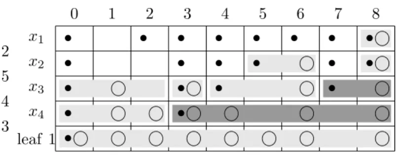
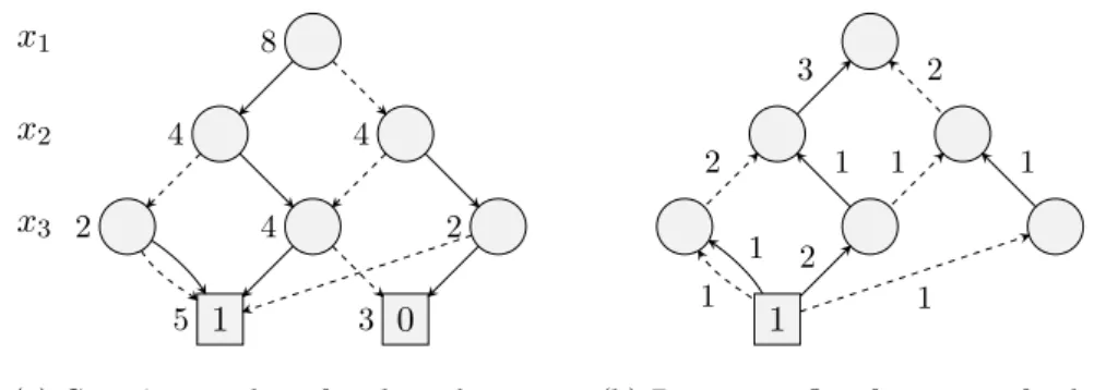
3.3. Variable order 25 x1 x2 x3 x4 leaf 1 2 5 4 3 0 1 2 3 4 5 6 7 8 • • • • • • • • • • • • • • • • • • • • •

Figure 3.3: Dynamic programming table for the linear constraint2x1+5x2+4x3+3x4 ≤8.

Variables Uln, Dln are shown as•, resp. The light grey blocks represent the nodes in

the ROBDD, and the dark grey blocks represent the redundant nodes in the QOBDD.

The last improvement in the series of exact minimization algorithms based on Friedman and Supowit's method was again achieved by Ebendt [Ebe03]. The expensive movements of variables through the BDD were substituted by a state expansion technique which signicantly reduced the runtime.

In [EGD04] Ebendt et al. broke new ground. They did not use Friedman and Supowit's approach any longer but combined the search algorithm A∗ known from articial intelli-gence with Branch & Bound. They reused the lower bound they had developed in [EGD03] and the state expansion technique presented in [Ebe03].

All of the known algorithms have in common that they need to build a BDD for the computation of an optimal variable order.

3.3.5 0/1 Integer Programming

Given a linear constraintaTx≤bin dimensiondwe want to nd an optimal variable order for building the corresponding threshold ROBDD. In the following we derive a 0/1 integer program whose solution gives the optimal variable order and the minimal number of nodes needed. It also forms the basis for the computation of the variable order spectrum of a threshold function in section 3.3.6. In contrast to all other exact BDD minimization techniques (see section 3.3.4), our approach does not need to build a BDD explicitly.

As we have seen in section 3.1, building a threshold BDD is closely related to solving a knapsack problem. A knapsack problem can be solved with dynamic programming [Sch86] using a table. We mimic this approach on a virtual table of size(d+ 1)×(b+ 1)which we

ll with variables. Figure 3.3 shows an example of such a table for a xed variable order. The corresponding BDD is shown in gure 3.1(a) on page 12.

W.l.o.g. we assume ∀i ∈ {1, . . . , d} ai ≥ 0, and to exclude trivial cases, b ≥ 0 and

Pd

i=1ai > b. Now we start setting up the 0/1 IP shown in gure 3.4. The 0/1 variables

yli (3.25) encode a variable order in the way thatyli= 1 i the variable xi lies on levell.

To ensure a correct encoding of a variable order we need that each index is on exactly one level (3.3) and that on each level there is exactly one index (3.4).

We simulate a down operation in the dynamic programming table with the 0/1 variables Dln (3.26). The variable Dln is 1 i there exists a path from the root to the levell such

min P l∈{1,...,d+1} n∈{0,...,b} Cln+ 1 (3.2) s.t. ∀i∈ {1, . . . , d} Pd l=1yli = 1 (3.3) ∀l∈ {1, . . . , d} Pd i=1yli= 1 (3.4) ∀n∈ {0, . . . , b−1} D1n= 0 (3.5) ∀l∈ {1, . . . , d+ 1} Dlb = 1 (3.6) ∀n∈ {1, . . . , b} U_(d+1)n= 0 (3.7) ∀l∈ {1, . . . , d+ 1} Ul0 = 1 (3.8) B(d+1)0= 1 (3.9) ∀n∈ {1, . . . , b} B(d+1)n= 0 (3.10) C(d+1)0= 1 (3.11) ∀n∈ {1, . . . , b} C_(d+1)n= 0 (3.12) ∀l∈ {1, . . . , d}: ∀n∈ {0, . . . , b−1} Dln−D(l+1)n≤0 (3.13) ∀n∈ {1, . . . , b} U(l+1)n−Uln≤0 (3.14) ∀n∈ {0, . . . , b}, j∈ {1, . . . , n+ 1} Dln+Ul(j−1)− Pn i=jUli−Bl(j−1) ≤1 (3.15) ∀l∈ {1, . . . , d}, i∈ {1, . . . , d}: ∀n∈ {0, . . . , b−ai} yli+Dl(n+ai)−D(l+1)n≤1 (3.16) ∀n∈ {b−ai+ 1, . . . , b−1} yli−Dln+D(l+1)n≤1 (3.17) ∀n∈ {0, . . . , b−ai} yli−Dl(n+ai)−Dln+D(l+1)n≤1 (3.18) ∀n∈ {ai, . . . , b} yli+U(l+1)(n−ai)−Uln≤1 (3.19) ∀n∈ {1, . . . , ai−1} yli−U(l+1)n+Uln≤1 (3.20) ∀n∈ {ai, . . . , b} yli−U(l+1)(n−ai)−U(l+1)n+Uln≤1(3.21) ∀n∈ {0, . . . , ai−1} yli+Bln−Cln≤1 (3.22) ∀n∈ {0, . . . , ai−1} yli−Bln+Cln≤1 (3.23) ∀n∈ {ai, . . . , b}, k∈ {n−ai+ 1, . . . , n} yli+Bln+B(l+1)k−Cln≤2 (3.24) ∀l∈ {1, . . . , d}, i∈ {1, . . . , d}: yli∈ {0,1} (3.25) ∀l∈ {1, . . . , d+ 1}, n∈ {0, . . . , b}: Dln, Uln∈ {0,1} (3.26) Bln, Cln∈ {0,1} (3.27)

Figure 3.4: 0/1 integer program for nding the optimal variable order of a threshold BDD for a linear constraintaT_{x≤bin dimension d.}