Full Terms & Conditions of access and use can be found at
https://www.tandfonline.com/action/journalInformation?journalCode=nurw20
Urban Water Journal
ISSN: 1573-062X (Print) 1744-9006 (Online) Journal homepage: https://www.tandfonline.com/loi/nurw20
Applying human mobility and water consumption
data for short-term water demand forecasting
using classical and machine learning models
Kamil Smolak, Barbara Kasieczka, Wieslaw Fialkiewicz, Witold Rohm,
Katarzyna Siła-Nowicka & Katarzyna Kopańczyk
To cite this article: Kamil Smolak, Barbara Kasieczka, Wieslaw Fialkiewicz, Witold Rohm, Katarzyna Siła-Nowicka & Katarzyna Kopańczyk (2020) Applying human mobility and water consumption data for short-term water demand forecasting using classical and machine learning models, Urban Water Journal, 17:1, 32-42, DOI: 10.1080/1573062X.2020.1734947
To link to this article: https://doi.org/10.1080/1573062X.2020.1734947
© 2020 The Author(s). Published by Informa UK Limited, trading as Taylor & Francis Group.
View supplementary material
Published online: 10 Mar 2020. Submit your article to this journal
Article views: 154 View related articles
RESEARCH ARTICLE
Applying human mobility and water consumption data for short-term water demand
forecasting using classical and machine learning models
Kamil Smolak a, Barbara Kasieczka a, Wieslaw Fialkiewicz b, Witold Rohm a, Katarzyna Siła-Nowicka c,d and Katarzyna Kopańczyk a
aInstitute of Geodesy and Geoinformatics, Wroclaw University of Environmental and Life Sciences, Wroclaw, Poland;bInstitute of Environmental Engineering, Wroclaw University of Environmental and Life Sciences, Wroclaw, Poland;cUrban Big Data Centre, University of Glasgow, Glasgow, UK; dSchool of Environment, University of Auckland, Auckland, New Zealand
ABSTRACT
Water demand forecasting is a crucial task in the efficient management of the water supply system. This paper compares classical and adapted machine learning algorithms used for water usage predictions including ARIMA, support vector regression, random forests and extremely randomized trees. These models were enriched with human mobility data to improve the predictive power of water demand forecasting. Furthermore, a framework for processing mobility data into time-series correlated with water usage data is proposed. This study uses 51 days of water consumption readings and over 7 million geolocated mobility records from urban areas. Results show that using human mobility data improves water demand prediction. The best forecasting algorithm employing a random forest method achieved 90.4% accuracy (measured by the mean absolute percentage error) and is better by 1% than the same algorithm using only water data, while classic ARIMA approach achieved 90.0%. The Blind (copying) prediction achieved 85.1% of accuracy.
ARTICLE HISTORY
Received 22 May 2019 Accepted 20 February 2020
KEYWORDS
Short-term forecasting; water demand; water consumption; geolocated data; classical forecasting; machine learning
1. Introduction
Water consumption prediction has recently become a very active field of study, as it leads to significant economic and environ-mental benefits (Brentan et al.2018). Accurate water demand prediction ensures a reliable water distribution system and pro-vides users with water in adequate volumes and reduced but sufficient pressure. Decreasing water pressure across the net-work not only improves energy efficiency through lower pump-ing energy consumption but also reduces the probability of network failures. Water demand predictions also help to identify leakages when observed consumption significantly differs from the forecasted water demand (Herrera et al. 2010). However, pressure reduction requires detailed knowledge of many water consumption factors.
There is a number of parameters affecting water consump-tions such as climate, seasonality, economy, urban design and demographics (March and Sauri2009; Wong, Zhang, and Chen
2010). Brentan et al. (2018) focused on water demand time series generation using a priori knowledge of water demand consump-tion and weather data such as temperature, precipitaconsump-tion and humidity. A similar set of exogenous variables was used by Al-Zahrani and Abo-Monasar (2015) in their study on daily water demand predictions in Al-Khobar, Saudi Arabia. Effects of includ-ing weather information were also investigated by Ghiassi, Zimbra, and Saidane (2008). Babel, Gupta, and Pradhan (2007) developed a model based on a multidimensional approach, using socio-economic characteristics, weather data, public water strategies and policies. Their results indicated that the demographic indicators, water tariffrate, public education level
and average annual rainfall are significant variables for predic-tions of domestic water demand. These factors and their spatial and temporal resolutions have varying significance depending on the prediction time horizon. There are four common types of these horizons used for water forecasting (Rinaudo2015): short-term forecasting (hours, days, weeks) is used to optimise a water supplying system; intermediate-term forecasting (1–10 years) is used for demand predictions that account for change in the number of consumers; long-term forecasting (20–30 years) is usually used when major changes in the system need to be planned, e.g. in desalination plants and for large-capacity inter-basin transfers.
The most commonly used predictive models for water demand forecasting comprise autoregressive integrated mov-ing average (ARIMA) and autoregressive integrated movmov-ing average with exogenous variables (ARIMAX) methods (Braun et al.2014; Alvisi, Franchini, and Marinelli2007). Recent studies, however, introduce machine learning (ML) solutions, such as Artificial Neural Networks (ANN), Support Vector Regression (SVR) and regression trees, which now outperform the classical methods (Herrera et al. 2010; Tiwari and Adamowski 2017; Bennett, Stewart, and Beal2013; Bai et al.2014; Donkor et al.
2014; Antunes et al.2018; Xu et al.2019).
Despite the increasing number of studies on water demand forecasting using exogenous variables and growing awareness of the significance of the human factor, most research omits population behaviour or assumes only the regular patterns (Wong, Zhang, and Chen2010; Alvisi, Franchini, and Marinelli
2007; Alcocer-Yamanaka, Tzatchkov, and Arreguin-Cortes
CONTACTKamil Smolak [email protected]
Supplemetary data for this article can be accessedhere. 2020, VOL. 17, NO. 1, 32–42
https://doi.org/10.1080/1573062X.2020.1734947
© 2020 The Author(s). Published by Informa UK Limited, trading as Taylor & Francis Group.
This is an Open Access article distributed under the terms of the Creative Commons Attribution-NonCommercial-NoDerivatives License (http://creativecommons.org/licenses/by-nc-nd/4.0/), which permits non-commercial re-use, distribution, and reproduction in any medium, provided the original work is properly cited, and is not altered, transformed, or built upon in any way.
2012). Since human water consumption accounts for a major proportion of water demand (Wong, Zhang, and Chen2010), ignoring or simplifying this variable may reduce the accuracy of water demand forecasts. To address this research gap, this paper aims to study the influence of exogenous variables related to human mobility on water demand forecasting using classical and machine learning methods.
Human mobility-related data consist of at least a set of coordinates and a timestamp, which may be used to recon-struct human movements and mobility patterns (Barbosa-Filho et al. 2018). These data are harvested from various sources, such as mobile phones, wearable cameras or GPS devices and provide very detailed spatial and temporal information. Human mobility data have been used in city planning (Barbosa-Filho et al.2018), traffic engineering (Toole et al.2015) and epide-miology (Bengtsson et al.2015). To the best of our knowledge, this research is afirst attempt of utilising the innovative geolo-cated data for public utilities demand forecasting.
The objective of this research is to propose an integrated approach for short-term water demand forecasting using histor-ical water consumption data in district metering areas (DMA) and human mobility data. This study compares the performance of classical forecasting methods and machine learning approaches for water demand prediction. The proposed approach is evalu-ated onfive different DMAs in the city of Wroclaw and includes data processing and aggregating, training the forecasting mod-els and validation. The merits and limitations of the applied methods are discussed and directions for further improvement of prediction accuracy are identified.
2. Materials and methods
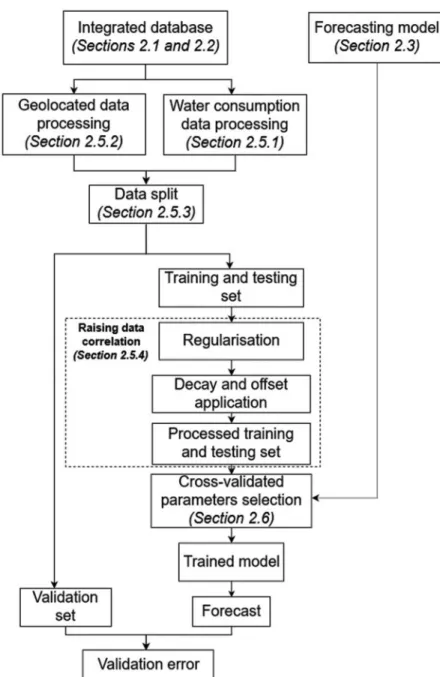
The forecasting framework designed for this research is pre-sented inFigure 1and it reflects the structure of this section. The data (historical water consumption readings and mobile phone data records) are stored and spatiotemporally inte-grated into a database. The developed model connects to the database to get the data required for the chosen time of pre-diction. The data are then automatically processed and fed into the training, testing and evaluation step. At the same time, one of the forecasting methods described inSection 2.3is tuned in an automated process to achieve the best possible model performance. Finally, the forecasted time-series are produced.
2.1. Study area
The study site is located in Wroclaw, the fourth largest city in Poland with a population of approximately 628,600 inhabitants, covering an area of nearly 293 km2. The water is supplied to 99% of citizens from two main water treatment plants. The distribution network is characterized by a great variance in age and material which results in over 10% losses (Fialkiewicz et al.2018). Annual energy consumption by the water supply system accounts for 19 GWh. Total Wroclaw’s annual water consumption in 2018 was 48.7 hm3. Water consumption data used in this project were shared by local water infrastructure manager MPWiK S.A. in a form of ten-minute readings of water consumption in the DMAs.
Mobile phone data were purchased from mobile marketing company Selectivv that scans over 200,000 mobile applications to harvest information about mobile phones location. These data are gathered at the time when the mobile app storing location history was on the list of active applications or was running as a background process. The database consists of 7,133,087 geolocated data records with information for every record about event registration time (timestamp), application name, device location and in some cases also user ID.
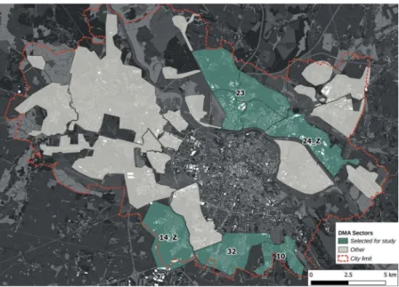
The historical water consumption readings and mobile phone data records cover a time range of 51 days, from 21stof January (Sunday) to 12thof March 2018 (Monday) (for the dataset plots see Appendix A). Due to low temperatures within the selected period water consumption corresponds mostly to in-house water usage observed in winter. There are twenty-eight DMAs in Wroclaw that cover 51% of the entire city area. However, a considerable part of the city is still unmetered and therefore, any uncontrolled change in daily water demand hinders the management of water supply system. This study analysesfive DMAs–labelled 10, 14_Z, 23, 24_Z, 32 which correspond to 34% of the total city hydraulic sectors area (Figure 2). The selected DMAs differ from each other by the predominant function of the buildings. Sectors 10, 14_Z and 32 are typical residential areas with around 80% of residential housing and less than 4% of industrial buildings. DMA 24_Z stands out with the highest percentage of the buildings with an industrial function which is 23% with only 45% of residential areas. Whereas, sector 23 accounts for a moderate percentage of residential and industrial areas. Consequently, population density also varies, ranging from ~3 000 inhabitants per km2in DMA 10 to less than 1000 inhabi-tants per km2 in DMA 24_Z. The number of geolocated data records in each DMA is higher in residential areas (DMA 32: 30%, DMA 14_Z: 22%, DMA 10: 20% of the data) than in industrial and mixed sectors (DMA 24_Z: 17%, DMA 23: 10%).
The diversity of the predominant function of DMAs is reflected in the water consumption characteristics and week cyclicity. In residential and mixed sectors, increased water con-sumption can be observed in the mornings and the evenings of each day. While in the industrial sector, consumption is much more irregular and reduces significantly during the weekend (21.01.2018–Sunday, 28.01.2018–Saturday).
2.2. Data preprocessing
To ensure maximum efficiency in data processing, a spatiotemporal database was created using the open-source database software PostgreSQL and its extensions: PostGIS for spatial data and TimescaleDB for time-series. All the data have to be transformed and loaded into a database predefined structure. This has to be done manually. Therefore, the model is independent of the structure of provided data. Furthermore, the data are aggregated spatially into DMAs and temporally to one-hour bins. If provided data (either water consumption or mobility data) have lower temporal resolution it can be aggre-gated to the larger bins. Similarly, if an infrastructure manager provides different spatial segmentation (i.e. DMAs), then the data are aggregated to the provided areas. The datasets used in this study were thoroughly tested for their reliability, represen-tativeness and consistency.
To correct the water consumption data, erroneous readings were eliminated and the time series were examined for continu-ity. Outliers were removed using the interquartile range rule. In this method interquartile range (IQR) is the difference between the third (Q3) andfirst quartile (Q1). Every value lower than Q1–
1.5 x IQR and higher than Q3 + 1.5 x IQR was eliminated. As
a result, in sectors 10, 14_Z, 23, 24_Z and 32 the percentage of eliminated readings was respectively: 0,1%, 0,8%, 1,1%, 6,7% and 10,3% of the available data. The main reason for the elimination was a meter failure resulting in empty consumption readings, which accounted for over 95% of the rejected records. The remaining 5% were erroneous readings, i.e. those with negative values and outliers. After the initial filtrations, data continuity tests were carried out to identify and describe the length and density of time series gaps. Based on time series continuity charts, 51 days (from 21st of January to 12th of March 2018) were selected for the study, during which the gap in the data on water consumption did not exceed 1 hour.
The mobile phone data did not show any significant outliers, therefore, to prevent information loss, the geolocated data were not pre-processed but loaded into the database in a raw format. After loading and filtration, the data were spatially linked to the corresponding DMAs.
2.3. Forecasting models
Over the last decade, machine learning algorithms were found being superior to other statistical methods as they are highly capable of handling nonlinear and imprecise data (Ghalehkhondabi et al.2017; Herrera et al.2010). Furthermore, machine learning algorithms architecture can be easily adjusted to employ multi-source data in a prediction task. This work compares a few popular machine learning regression methods (Support Vector Regression (SVR) and ensemble tree-based methods) with ARIMA and ARIMAX models. As a simulation of lower bound of predictability, a Blind approach is employed.
2.3.1. ARIMA
Auto-regressive integrated moving average model (ARIMA) (Box et al.2015) is a classical forecasting model which combines auto-regressive (AR) and moving average (MA) components with additional time-series differencing (I). ARIMA is defined as follows:
ϕpð ÞðB tBÞ d
Xt¼θqð ÞB at (1) where ϕ and θ are coefficients related to the AR and MA components respectively, estimated during a model fitting step. The Xt are the time-series elements at the time t and
aare the residuals,Bis a backshift expression used to denote previous elements or coefficients (named lags), hence
Bq¼X
tq. ARIMA orders (parameters)p andq determine the
number of previous lag observations taken into consideration when estimating model coefficients for AR and MA compo-nents anddis a number of differencing transformations, that is an order of lag subtracted from current elementXt.
Performance of a forecasting model can be improved by using additional information related to a predicted series. Such data are referred to as exogenous variables. ARIMA can be extended by adding such variables to the model. If we denote externalkinputs asxtk, then ARIMAXðp;d;qÞis defined as:
ϕpð ÞðB tBÞ d
Xt¼θqð ÞB aEtþ Xk
i¼1ηχi (2)
where η are the coefficients of external inputs estimated at a modelfitting step.
ARIMA and ARIMAX models have been used for decades and valued for their accuracy (Braun et al.2014; Alvisi, Franchini, and Marinelli 2007). Various extensions of the models were proposed, one of which are SARIMA (seasonal ARIMA) models that account for seasonal effects approximated from the past data, improving their accuracy in long-term forecasting. Despite a large number of studies showing the superiority of machine learning based methods over these models, some studies show that ARIMA and ARIMAX models are still more
accurate in long-term predictions than machine learning meth-ods (Ghalehkhondabi et al.2017).
2.3.2. Support vector machines
Support Vector Machines (SVMs) (Cortes and Vapnik1995) are supervised machine learning methods. Support Vector Regression is the adoption of SVMs for regression problems. The idea of SVR is to fit a p-1 dimensional hyperplane to a given set of points inpdimensional space by minimising the loss function, which ignores errors yielded by points lying within a margin of tolerance (defined by theεvalue). To support non-linear regression problems, the kernel function is used to trans-form the data into a higher dimensional feature space where a linear regression can be performed. In comparison to tradi-tional regression procedures, SVR attempts to minimize the pre-diction error bound to achieve generalized performance, instead of minimizing the observed training error. Over the last decade, a lot of research has been done to improve the SVR in water demand predicting task, finding it resistant to overfitting and having a lower error on previously unseen data, which is impor-tant for the noisy water consumption data (Ghalehkhondabi et al.2017). The limitation of SVR is that the algorithm perfor-mance is vulnerable to parameters choice. In order to overcome this problem hybrid SVR with externally determined parameters can be implemented (Bai et al.2014).
2.3.3. Tree-based ensemble methods
This is a class of supervised learning algorithms based on a tree structure, which can be used for regression problems. In ensemble methods, during the treefitting process, a large collection of trees is constructed. Then, the result is computed as an average from the results of each tree. With the ability to model nonlinear relationships and resistance to overfitting, tree-based ensemble methods were applied for water demand forecasting producing better results than other machine learning algorithms (Chen et al.
2017; Herrera et al. 2010; Tyralis, Papacharalampous, and Langousis2019). Furthermore, the tree-based ensemble methods
can effectively handle small sample sizes, which is important in the case of limited data availability. Among the significant limitations of this group of methods is their inability to extrapolate outside the range of a training sample (Tyralis, Papacharalampous, and Langousis2019).
Random forests (RF) (Breiman2001) learn a set of trees, where the training algorithm applies bootstrap aggregation (also known as bagging) to each learner which means that each new tree is constructed using randomly selected chunk of the data. In RF, a decision of the best node split, which minimises an internal error criterion, is made using a random subsample from an already selected fragment of a learning set. This leads to the creation of a series of uncorrelated trees, which individually are weak predic-tors. Then, a new sample is run through each of the trained trees. Because of a random characteristic of data subsample selection some data are not used to construct trees. These samples create an‘out-of-bag’dataset, which is used to evaluate the model and rebuild it with tuned parameters if needed. This procedure yields better results and prevents model overfitting.
Extremely randomized trees, called also Extra-Trees (ET) (Geurts, Ernst, and Wehenkel2006) are also based on the bag-ging approach. The difference is that the whole dataset is used to train trees and a random selection of samples is applied at the node-splitting step, where a cutting point is selected at random from selected features. The node-splitting process stops only when the output is constant or the number of elements is lower than the selected value. From the bias-variance point of view, the strongly randomized approach reduces variance better than other algorithms, while using the whole sample for each tree construction minimises its bias.
2.3.4. Blind approach
The Blind approach is used to determine the lower bound of predictability and as a reference for any other algorithm. It is defined as:
Xt¼Xt168h: (3)
whereXtis the predicted water demand at timetandXt168h is the reading from exactly one week earlier.
2.4. Model validation
The results were evaluated using commonly known assessment methods. As a prediction accuracy measures, a mean absolute percentage error measure (MAPE), root mean squared error (RMSE) and Nash-Sutcliffe index of efficiency (EI) were used. If we denotenas a number of compared values,yi as the original value of water consumption from the test or validation set,^yi as the water demand prediction andy as the mean value of the observations, then the measures are defined as follows (Donkor et al.2014): MAPE ¼ 100% n Xn i¼1 yi^yi j j yi j j ; (4) RMSE¼ ffiffiffiffiffiffiffiffiffiffiffiffiffiffiffiffiffiffiffiffiffiffiffiffiffiffiffiffiffiffiffiffiffiffiffi 1 n Xn i¼1ðyi^yiÞ 2 r ; (5) EI¼1 Pn i¼1ðyi^yiÞ 2 Pn i¼1ðyiyÞ2 ; (6)
The MAPE expresses a relative error which is comparable between different time-series. When it equals zero, then the prediction is identical to real water usage. The RMSE is sensitive to outliers and when equals to zero, the model fit data per-fectly. It cannot be compared between time-series as it is not normalised. The EI expresses the goodness offit of a model and is more sensitive to systematic errors (Herrera et al.2010). The EI can range from -∞ to 1 inclusively. When EI = 1 the model perfectlyfits the data.
The mean squared error (MSE) and mean absolute error (MAE) metrics were used as a split evaluation criterion in tree-based models. These are defined as:
MSE ¼ 1 n Xn i¼1ðyi^yiÞ 2; (7) MSE ¼ 1 n Xn i¼1jyi^yij; (8)
We use the autocorrelation function (ACF) and the partial auto-correlation function (PACF) for an initial determination of ARIMA and ARIMAX orders and validation of results. Autocorrelation is defined as the correlation between an ele-ment of a signal with its lag. Therefore, the autocorrelation ofn
lag is a correlation between elementsXtandXtn. Partial auto-correlation is a auto-correlation between a signal with its own lagged values, where linear dependence for shorter lags are removed. ARIMA and ARIMAX orders were selected using Akaike’s Information Criterion (AIC) which is a commonly used measure for classical forecasting models (Anele et al.2017). It is defined as:
AIC¼2n2nll; (9)
wherenis a number of estimated parameters in the model and
nllis a log-likelihood function for the model. It is the metric of relative model quality on the same set of data. The model with the lowest value of AIC is considered the best.
2.5. Data processing
The pre-processed water use readings and mobile phone data are integrated into a database and must undergo further proces-sing to improve the quality and structure of the data to more accurately predict urban water use. Each prediction is made using the period of 21-days of the data selected from the whole dataset.
2.5.1. Water consumption data processing
The filtered and pre-processed water consumption data are analysed to identify potential trends and week cyclicity effects which help to select the best parameters for forecasting mod-els. To adjust to the temporal resolution of the mobile phone data, ten-minute readings are summed into one-hour periods. Any data gaps are identified andfilled with the closest present reading from the same hour and day of a week.
2.5.2. Geolocated data processing
In order to use geolocated data as an exogenous predictor, transformation into time-series is required. As the mobile phone data are loaded into the database in a raw format, depending on the application, data may require selectivefi ltra-tion. For example, some mobile applications are programmed to automatically record a person’s mobile phone position at midnight and, as this is not a common time for water consump-tion activity, these records are removed from the database. After filtering out useless records, the data are aggregated into one-hour bins for each DMA in the study area, where the total number of records per DMA is counted. This operation creates a time-series for each of the DMAs.
2.5.3. Data split
The water consumption and the processed geolocated data are merged and split into two datasets: 14 days of learning and testing sets and 7 days of validation data (66.7% and 33.3% respectively). The learning and testing data are taken together and shuffled during the 3-fold cross-validation process for model parameters tuning (Section 2.6), while the validation dataset is used only once at the end of the forecasting process. N-fold cross-validation divides data n-times into learning and testing sets, which are used to train and evaluate tested models. This approach allows to achieve more reliable results through multiple repetitions of the learning-testing process and to detect overfitting at an early stage. Due to its individual time-series characteristics, the modified cross-validation pro-cess is implemented for this work. The previously pre-selected days are split using a moving time window which randomly selects a starting point at least two weeks before the last date in the training and testing dataset. The cross-validation results are calculated as an average from the test scores of each fold. 2.5.4. Raising data correlation
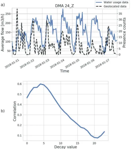
A high correlation between the geolocated data and water consumption time-series indicates their similarity. Therefore, the exogenous variable would potentially improve the forecast-ing accuracy if that variable is highly correlated with the pre-dicted series. To maximise series correlation, the mobility data need to be processed each time when prediction has to be done. First, due to the temporal sparsity of the data, records from the whole training period are accumulated and averaged with respect to the days of the week. This creates a pattern of a‘typical week’for each of the studied DMAs. After that, the geolocated series is controlled by two parameters named decay and offset. The former informs how long a single record is accounted for, that is, if a mobile phone logs at a specific time, for non-zero decay values it will be still considered to be in an area for the determined period. The offset parameter shifts the geolocated series by a given value, so if the applica-tion creates a log just before a person arrives home, that would align mobile phone records with the water demand series (Figure 3(a)). These parameters are selected individually for each DMA during the model training phase through the exhaustive procedure. Parameters are learned only using the training data but are applied further throughout testing and validation phases. For each value of decay parameter, the offset that maximises the correlation of the geolocated series and the
water consumption series is determined by the convolution of their Fourier transforms. The inverse Fourier transform is con-sidered to be equal to the calculation of correlation of these series for every possible offset parameter. The combination of these two parameters with the highest series correlation value is selected. This procedure allows raising the correlation level to a range of 40%–75%. (Figure 3(b)) and increase computational efficiency.
2.6. Model parameters selection
Each tested algorithm has its unique parameters determining its behaviour. Before training, the model automatically searches for the best parameters’combination for a current prediction. This is done by a searching algorithm which uses a predefined set of parameters tofit the model and selects the combination of these parameters giving the lowest error. The best para-meters’ combination is then used to validate the model. Results from the validation are presented inSection 3. 2.6.1. ARIMA and ARIMAX model tuning
First, predefined set of ARIMA and ARIMAX orders p (from 1 to 5), d (from 0 to 2), and q (from 1 to 5) is determined using ACF and PACF functions. Next, every possible combination of these parameters is tested by an exhaustive grid search algo-rithm which fits model to the training and testing data. The model with the lowest value of AIC is selected.
In classical approaches, cyclicity has to be determined expli-citly for the algorithm. The seasonal pattern is modelled by the spline basis function (De Boor1978) using current training set and is given as an exogenous variable. This approach captures the cyclicity of the data a priori and does not raise the complex-ity of the calculations.
2.6.2. Machine learning methods tuning
The tested ML methods’initial parameters (called hyperpara-meters) have to be set up before running the algorithm and can significantly affect a model’s performance. For each of the algorithms, the best performing combination is selected using a random search and a training and testing dataset with 3-fold cross validation applied. It works similarly to the grid search method (2.6.1) but onlynrandom combinations are selected. In this case, 100 combinations are tested every time.
Tree-based models are tested for a number of trained trees (from 10 to 1000) and a type of split evaluation criterion (MSE or MAE). The SVR model is tested for various types of kernels (linear, sigmoid, radial basis function, polynomial), various epsi-lon values (from 10−4to 10) and a penalty parameter C (from 10−3to 20). The epsilon value determines the threshold of an acceptable error where no penalty is given during the training process. The penalty parameter is used to control the trade-off between bias and overfit.
The machine learning methods were adapted for time-series forecasting, which required creating internal and external lag parameters. These lags define how many previous records (hours) from the data are considered at each prediction step. Internal lag determines the number of water demand readings considered and external lag controls the number of geolocated data records fed into the model.
Experimental calculations showed that MAPE drops for 24 and again for 168 lags, which is the length of a day and a week (in hours), respectively. The value of 168 lags is used for every prediction. After setting the number of internal lags, the same test is run for a number of external lags. However, for that parameter, the prediction accuracy does not vary significantly, since the external data are provided in real-time. Hence, 5 lags for geolocated data were used as it guarantees robustness for missing data in most cases and is low enough not to raise the complexity of calculations.
3. Results and discussion
Due to the heuristic nature of machine learning algorithms, it is important to ensure the multiple validation of the models on various time ranges. Experimental results were calculated in a validation process which was repeated 30 times, each time selecting 21 consecutive days of data from the whole study period of 51 days with a 24-hours step. Finally, errors were averaged from all the validation cases. For each method, diff er-ent variants of fed data were calculated. The results for 7-days and 24-hours forecasts are presented inTables 1and2(for the separate results for each DMA see Appendix B). W indicates that historical water consumption data were used. The geolo-cated data are abbreviated as G. If a decay parameter was applied it is denoted asDand if time-series where shifted by
an offset parameter it is denoted asO. Hence, when geolocated data were processed by decay and offset parameter it is abbre-viated as G(D,O) and when data were not processed it is denoted as G. The geolocated data modified using only the offset parameter is denoted asG(O).
3.1. Weekly forecasts
Table 1shows that the Blind prediction method, for a weekly forecast, has an accuracy (measured as 1 – MAPE) of almost 85%, which means that most of the long-term trends in the water demand are rather cyclic-based than week-based. Therefore, all the methods that contain cyclic-signal will be correct. Comparing all the other methods to the Blind approach reveals that the gained improvements are on the level of 20% for EI, 40% RMSE and up to 35% for MAPE.
Following this major notion that the cyclic variation plays a central role in water demand signal it is also clear to observe that classical autoregressive prediction methods such as ARIMA and ARIMAX provide second best predictions and are insensi-tive, i.e. they do not take any advantage of exogenous variable– geolocated data. It looks as the impact of such data contains too scattered, non-seasonal signal that is difficult to model using polynomials (Equation (2)).
The sole use of geolocation data (G inTable 1) provides less predictive accuracy than any other tested data source (Blind
Figure 3.Correlation of geolocated data and water usage time-series in DMA 24_Z: (a) series comparison after applying offset and decay parameters. (b) correlation depending on the decay parameter for each DMA. Depicted correlations are calculated for the best offset parameter.
approach in terms of MAPE). It is, however, providing an advan-tage when looking into the RMSE and EI parameters. These results show that the seasonal variation in the geolocation data were not pertaine, but a short term scatter would be well represented.
If one would like to compare machine learning methods (ET, RF, SVR) applied with or without geolocation data, it is clear that these data slightly change forecasts and the most success-ful uptake of such data improves forecasts by 1.4%. Moreover, increase in correlation between G and W time series as shown in thesection 2.5.2. is not always improving forecasting skills of the algorithms (seeTable 1e.g. RF RMSE W + G vs W + G(D,O)).
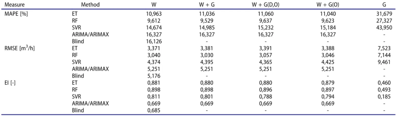
3.2. 24-hours forecasts
Results inTable 2show that for a 24-hours prediction the Blind method provides better estimates of the water demand than the one based on geolocation data only (G), but interestingly it also outperforms in all cases of ARIMA/ARIMAX approach. The other results shown in Table 2are consistent with these pre-sented inTable 1. Random forest approach works best based on all three statistics and adding geolocation data is improving solution only by a single percentage. It might suggest that for a shorter forecast horizon the cyclical term is less determining than for longer forecasts, hence the machine learning approaches (ET, RF, SVR) work better than standard predictive models and the Blind method.
3.3. Classical and machine learning water demand prediction methods
Results inTables 1and2indicate that the RF proved to be the best performing method for all the DMAs which is consistent with the results presented by Antunes et al. (2018). Yet, their analyses use a set of additional input features such as tempera-ture and rain occurrences, which may cause different and incom-parable results. Errors yielded by ARIMA/ARIMAX and ET algorithms are very similar to each other and 0.5% higher on average than the RF results. In accordance with Antunes et al. (2018) and Xu et al. (2019), the SVR algorithm performs worse than other models. Its performance results are similar to the Blind method. Also, Ghalehkhondabi et al. (2017) in the review paper point out that the machine learning (named soft computing methods) are outperforming classical multilinear regression, multiple non-linear regression and ARIMA methods. Literature review (Braun et al.2014; Chen et al.2017; Antunes et al.2018) offers usually a comparison of shorter forecasts: daily water demand/use (one value per day) or sub-daily prediction (24 values per day). In these studies SVR (Braun et al.2014) is out-performing SARIMA by 1% (1-sigma) and 4% (2-sigma) (mea-sured as a percentile relative error). Antunes et al. (2018) present a comparison of models where ARIMA is outperformed by RF and ANN by 50% in terms of MAPE and 5% of RMSE. In another study (Adamowski et al. 2012) RMSE of ARIMA is two times higher than the best performing ANN method. It has to be mentioned that the weekly forecast is not usually validated
Table 1.Calculated average MAPE, RMSE and EI for 7-days ahead forecast for all the DMAs with respect to the methods and variants.
Measure Method W W + G W + G(D,O) W + G(O) G
MAPE [%] ET 10,044 10,071 10,056 10,075 19,891 RF 9,611 9,558 9,601 9,601 17,769 SVR 14,232 14,065 14,146 14,187 39,166 ARIMA/ARIMAX 9,969 9,969 9,969 9,969 -Blind 14,934 - - - -RMSE [m3/h] ET 3,476 3,474 3,480 3,479 5,271 RF 3,369 3,355 3,368 3,366 5,098 SVR 4,509 4,447 4,380 4,433 8,637 ARIMA/ARIMAX 3,523 3,523 3,523 3,523 -Blind 5,798 - - - -EI [-] ET 0,886 0,885 0,885 0,885 0,753 RF 0,888 0,889 0,888 0,888 0,764 SVR 0,809 0,813 0,813 0,813 0,361 ARIMA/ARIMAX 0,863 0,863 0,863 0,863 -Blind 0,688 - - -
-Table 2.Calculated average MAPE, RMSE and EI MAPE for 24-hours ahead forecast for all the DMAs with respect to the methods and variants.
Measure Method W W + G W + G(D,O) W + G(O) G
MAPE [%] ET 10,963 11,036 11,060 11,040 31,679 RF 9,612 9,529 9,637 9,623 27,327 SVR 14,674 14,985 15,232 15,184 43,950 ARIMA/ARIMAX 16,327 16,327 16,327 16,327 -Blind 16,126 - - - -RMSE [m3/h] ET 3,371 3,381 3,391 3,388 7,523 RF 3,040 3,030 3,057 3,046 7,144 SVR 4,374 4,395 4,365 4,425 9,461 ARIMA/ARIMAX 5,251 5,251 5,251 5,251 -Blind 5,176 - - - -EI [-] ET 0,881 0,880 0,880 0,879 0,460 RF 0,898 0,898 0,896 0,897 0,493 SVR 0,811 0,801 0,788 0,794 0,185 ARIMA/ARIMAX 0,669 0,669 0,669 0,669 -Blind 0,685 - - -
-against the reference data (House-Peters and Chang2011) but such studies are suggested (Ghalehkhondabi et al.2017).
3.4. Autocorrelation function analysis
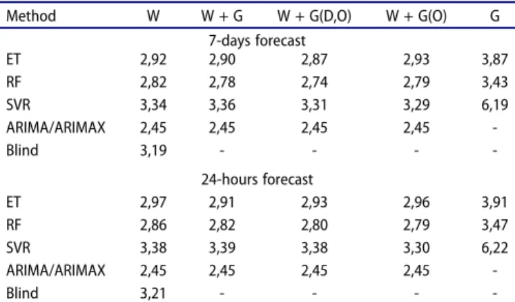
Additionally, the analysis of an ACF function on residuals was performed. In general, lower autocorrelation means that cyclic patterns and time-dependent relations have been captured and reproduced accurately. This usually leads to higher accu-racy of predictions. The degree of residuals’autocorrelation is expressed as an averaged share of statistically significant cor-relation values. It is presented in Table 3for 7-days and 24-hours forecasts.
Table 3 shows that the average share of significant cor-relation values for both forecasting horizons is the lowest for the ARIMA/ARIMAX method which indicates that this method captures time-dependent relations best, despite the fact it is not the best performing one. This can be caused by the explicit modelling of the cyclic pattern in this method. The tree-based ensemble approaches have a slightly higher share of significant correlations in ACF function than ARIMA/ARIMAX approach, with RF approach being the best ML method, which is consistent with the presented prediction errors (Tables 1 and 2). On the other hand, SVR performed the worst of all methods, including Blind approach, demonstrating the inability of this approach to effectively model cyclic patterns in the data. In a shorter forecasting horizon all the ML methods are performing worse than for 7-days ahead prediction, while classical approach has the same amount of statistically significant correlation values in the ACF function.
Importantly, when geolocation data were applied along with W time series in the ML methods, the average share of significant correlation values drops slightly (up to 3%) with the W + G(D, O) combination providing the largest decrease. Presumably, the geolocation data helps model dynamic fluctuations of cyclic patterns generated through an alternation of the human factor in water consumption. The ARIMA/ARIMAX methods were not affected by the geo-location data, therefore it does not influence the ACF func-tion of residuals.
3.5. Geolocated data application
The forecasts based only on the geolocation data are not captur-ing time-dependent relations, leadcaptur-ing to worse performance. However, if it was possible to model cyclic patterns a priori it may significantly improve the effectiveness of this method.
Results presented inTables 1–3show that adding geolocated data as exogenous variable slightly improves the accuracy of ML methods and has the largest impact for the longer forecast hor-izon. Moreover, adding geolocation data reduces the number of significant correlation values in the ACF function of residuals. For the best performing method, the average MAPE improves by over 0.9%.
The implication of improved 24-hours predictions on water supplying system has the potential to reduce energy costs. It was shown that using accurate water demand forecasting in energy optimization of the water pumping system can reduce energy consumption for about 39.4% (Bouach and Benmamar2019).
In comparison to other studies that used exogenous variables for water demand prediction, the accuracy gains are similar. Many water demand prediction models incorporate weather variables as an exogenous data as it has a large impact on prediction accuracy. Antunes et al. (2018) used temperature and rain information to predict water demand, achieving 0.25% MAPE improvement in the best case but at the same time they noted an increase of RMSE. Ghiassi, Zimbra, and Saidane (2008) improved MAPE of hourly forecasting model by 0.35% through adding weather infor-mation to the prediction. Al-Zahrani and Abo-Monasar (2015) did not provide a direct evaluation of the impact of adding weather information to prediction but they found MAPE to be varying by 0.71% depending on the types of variables used.
The geolocated data from mobile applications used in this study proved to be a useful addition for improved accuracy. Hence, to improve the model performance further, other more accurate human mobility data such as Call Detail Records and/or GPS data would have to be used. Future research will focus on more sophisticated utilisation of geolocated data and possible accuracy improvements. For instance, it is possible to classify geolocated data into trips and stops and to infer a purpose of a particular trip (Siła-Nowicka et al.2016) and then link it to an individual water usage profile, which may result in a better performance of forecasting models. Incorporating other datasets such as weather conditions or land use data could further improve model accuracy (Stańczyk et al.2018; Ghiassi, Zimbra, and Saidane2008; Al-Zahrani and Abo-Monasar2015).
4. Conclusions
The most important factor for a reliable and efficient water distribution system is providing an adequate volume of water at a reasonable pressure to its users. Therefore, short-term water demand forecasting is a crucial task in efficient water supply system planning and management.
This research studied the relationships between human mobi-lity-related data and information about approximate forecasted water demand. The experiment was conducted on data from the city of Wroclaw in Poland during winter, a time of in-house water usage. The selected DMAs have mixed characteristics: the DMA 10, 14_Z and 32 are predominantly residential, DMA 24_Z is an
Table 3.Averaged share of significant correlation values in the autocorrelation function for 7-days and 24-hours ahead forecasts for all the DMAs with respect to the methods and variants.
Method W W + G W + G(D,O) W + G(O) G 7-days forecast ET 2,92 2,90 2,87 2,93 3,87 RF 2,82 2,78 2,74 2,79 3,43 SVR 3,34 3,36 3,31 3,29 6,19 ARIMA/ARIMAX 2,45 2,45 2,45 2,45 -Blind 3,19 - - - -24-hours forecast ET 2,97 2,91 2,93 2,96 3,91 RF 2,86 2,82 2,80 2,79 3,47 SVR 3,38 3,39 3,38 3,30 6,22 ARIMA/ARIMAX 2,45 2,45 2,45 2,45 -Blind 3,21 - - -
-industrial area and DMA 23 is a mixed residential--industrial area. The proposed approach is thefirst application of human mobility data in water demand prediction models. It also evaluates the ability of predicting water demands using only human mobility data, which may be a promising opportunity for water infrastruc-ture managers who cannot afford to install meters on their net-work. With that, they still may be able to predict hourly urban water demand.
In this paper, the performance of classical and machine learn-ing algorithms was compared. The selected methods were ARIMA, SVR, RF, ET and the Blind approach. The paper proposes a forecasting framework and describes the full workflow, starting with data cleaning andfiltering, through geolocated and water demand data processing, to model training, tuning and evalua-tion. All of the tests were carried out with 3-fold cross-validation, using a different training and testing sample each time and validating the trained model once on the validation set.
The best performing algorithm was RF, reaching 90.4% pre-diction accuracy at an average for one-week ahead forecast. ET, which are also a tree-based algorithm, and classical regression methods had a slightly higher prediction error (4% on average). SVR performed worse than other methods and only slightly better than the blind approach. It was found that the autocor-relation of residuals was best minimised by the tree-based methods when exogenous data were used. Importantly, it was found that when human mobility data were incorporated into the model, statistical errors were lower and residuals were less correlated. It was also shown that the moderate (over 50%) correlation of the geolocated time-series and water demand data could be achieved through the introduction of decay and offset parameters, used for the human mobility data modifi ca-tion, which opens up the potential to use it as a water use predictor in the future. The future smart water supply manage-ment system could include a short-term prediction based on people mobility to locally adjust the pressure in the area where the large relocation of users is predicted or detected.
Acknowledgements
This work was carried out within the Climate-KIC’s Pathfinder Programme under Grant [number TC2018A_2.1.3-CHASE_P127-1A] supported by the EIT, a body of the European Union. The paper presents part of the results of the project CHASE: Citizens’ behaviour patterns for smart utilities and service management. The authors wish to thank the Selectivv Mobile House company and Municipal Water and Sewerage Company (MPWiK) for sharing the data for this study.
Disclosure statement
No potential conflict of interest was reported by the author(s).
Funding
This work was supported by the Climate-KIC [Citizens’behaviour patterns for smart utilities] under Grant [number TC2018A_2.1.3-CHASE_P127-1A].
ORCID
Kamil Smolak http://orcid.org/0000-0001-9113-6090 Barbara Kasieczka http://orcid.org/0000-0002-7858-4355
Wieslaw Fialkiewicz http://orcid.org/0000-0002-2517-5064 Witold Rohm http://orcid.org/0000-0002-2082-6366
Katarzyna Siła-Nowicka http://orcid.org/0000-0002-1850-1765 Katarzyna Kopańczyk http://orcid.org/0000-0002-5823-5537
References
Adamowski, J., H. Fung Chan, S. O. Prasher, B. Ozga-Zielinski, and A. Sliusarieva. 2012. “Comparison of Multiple Linear and Nonlinear Regression, Autoregressive Integrated Moving Average, Artificial Neural Network, and Wavelet Artificial Neural Network Methods for Urban Water Demand Forecasting in Montreal, Canada.” Water Resources Research48 (1). doi:10.1029/2010WR009945.
Alcocer-Yamanaka, V. H., V. G. Tzatchkov, and F. I. Arreguin-Cortes. 2012.
“Modeling of Drinking Water Distribution Networks Using Stochastic Demand.”Water Resources Management26 (7): 1779–1792. doi:10.1007/ s11269-012-9979-2.
Alvisi, S., M. Franchini, and A. Marinelli.2007.“A Short-term, Pattern-based Model for Water-demand Forecasting.”Journal of Hydroinformatics9 (1): 39–50. doi:10.2166/hydro.2006.016.
Al-Zahrani, M. A., and A. Abo-Monasar. 2015. “Urban Residential Water Demand Prediction Based on Artificial Neural Networks and Time Series Models.” Water Resources Management 29 (10): 3651–3662. doi:10.1007/s11269-015-1021-z.
Anele, A. O., Y. Hamam, A. M. Abu-Mahfouz, and E. Todini.2017.“Overview, Comparative Assessment and Recommendations of Forecasting Models for Short-term Water Demand Prediction.” Water 9 (11): 887. doi:10.3390/ w9110887.
Antunes, A., A. Andrade-Campos, A. Sardinha-Lourenço, and M. S. Oliveira. 2018. “Short-term Water Demand Forecasting Using Machine Learning Techniques.”Journal of Hydroinformatics20 (6): 1343–1366. doi:10.2166/ hydro.2018.163.
Babel, M., A. D. Gupta, and P. Pradhan.2007.“A Multivariate Econometric Approach for Domestic Water Demand Modeling: An Application to Kathmandu, Nepal.” Water Resources Management 21 (3): 573–589. doi:10.1007/s11269-006-9030-6.
Bai, Y., P. Wang, C. Li, J. Xie, and Y. Wang.2014.“Dynamic Forecast of Daily Urban Water Consumption Using a Variable-structure Support Vector Regression Model.”Journal of Water Resources Planning and Management 141 (3): 04014058. doi:10.1061/(ASCE)WR.1943-5452.0000457.
Barbosa-Filho, H., M. Barthelemy, G. Ghoshal, C. R. James, M. Lenormand, T. Louail, R. Menezes, J. J. Ramasco, F. Simini, and M. Tomasini.2018.
“Human Mobility: Models and Applications.”Physics Reports734: 1–74. doi:10.1016/j.physrep.2018.01.001.
Bengtsson, L., J. Gaudart, X. Lu, S. Moore, E. Wetter, K. Sallah, S. Rebaudet, and R. Piarroux.2015.“Using Mobile Phone Data to Predict the Spatial Spread of Cholera.”Scientific Reports5. doi:10.1038/srep08923. Bennett, C., R. A. Stewart, and C. D. Beal.2013.“Ann-based Residential Water
End-use Demand Forecasting Model.”Expert Systems with Applications 40 (4): 1014–1023. doi:10.1016/j.eswa.2012.08.012.
Bouach, A., and S. Benmamar.2019.“Energetic Optimization and Evaluation of a Drinking Water Pumping System: Application at the Rassauta Station.”Water Supply19 (2): 472–481. doi:10.2166/ws.2018.092. Box, G. E., G. M. Jenkins, G. C. Reinsel, and G. M. Ljung.2015.Time Series
Analysis: Forecasting and Control. Hoboken, New Jersey: John Wiley & Sons. Braun, M., T. Bernard, O. Piller, and F. Sedehizade.2014.“24-hours Demand Forecasting Based on SARIMA and Support Vector Machines.”Procedia Engineering89: 926–933. doi:10.1016/j.proeng.2014.11.526.
Breiman, L. 2001. “Random Forests.” Machine Learning 45 (1): 5–32. doi:10.1023/A:1010933404324.
Brentan, B. M., G. L. Meirelles, D. Manzi, and E. Luvizotto. 2018. “Water Demand Time Series Generation for Distribution Network Modeling and Water Demand Forecasting.”Urban Water Journal15 (2): 150–158. doi:10.1080/1573062X.2018.1424211.
Chen, G., T. Long, J. Xiong, and Y. Bai. 2017. “Multiple Random Forests Modelling for Urban Water Consumption Forecasting.”Water Resources Management31 (15): 4715–4729. doi:10.1007/s11269-017-1774-7. Cortes, C., and V. Vapnik. 1995. “Support-vector Networks.” Machine
De Boor, C.1978.A Practical Guide to Splines, 325. Vol. 27. New York: Springer. Donkor, E. A., T. A. Mazzuchi, R. Soyer, and A. J. Roberson.2014.“Urban Water Demand Forecasting: Review of Methods and Models.”Journal of Water Resources Planning and Management 140 (2): 146–159. doi:10.1061/(ASCE)WR.1943-5452.0000314.
Fialkiewicz, W., E. Burszta-Adamiak, A. Kolonko-Wiercik, A. Manzardo, A. Loss, C. Mikovits, and A. Scipioni. 2018. “Simplified Direct Water Footprint Model to Support Urban Water Management.”Water10 (5): 630. doi:10.3390/w10050630.
Geurts, P., D. Ernst, and L. Wehenkel.2006.“Extremely Randomized Trees.” Machine Learning63 (1): 3–42. doi:10.1007/s10994-006-6226-1. Ghalehkhondabi, I., E. Ardjmand, W. A. Young, and G. R. Weckman.2017.
“Water Demand Forecasting: Review of Soft Computing Methods.” Environmental Monitoring and Assessment 189 (7): 313. doi:10.1007/ s10661-017-6030-3.
Ghiassi, M., D. K. Zimbra, and H. Saidane. 2008. “Urban Water Demand Forecasting with a Dynamic Artificial Neural Network Model.”Journal of Water Resources Planning and Management 134 (2): 138–146. doi:10.1061/(ASCE)0733-9496(2008)134:2(138).
Herrera, M., L. Torgo, J. Izquierdo, and R. Pérez-García.2010.“Predictive Models for Forecasting Hourly Urban Water Demand.” Journal of Hydrology387 (1–2): 141–150. doi:10.1016/j.jhydrol.2010.04.005. House-Peters, L. A., and H. Chang.2011.“Urban Water Demand Modeling:
Review of Concepts, Methods, and Organizing Principles.” Water Resources Research47 (5). doi:10.1029/2010WR009624.
March, H., and D. Sauri.2009.“What Lies behind Domestic Water Use? A Review Essay on the Drivers of Domestic Water Consumption.” Boletin de la Asociacion de Geografos Espanoles50 (50): 297–314. Rinaudo, J.-D. 2015. “Long-term Water Demand Forecasting.” In
Understanding and Managing Urban Water in Transition. Global Issues in
Water Policy, Vol 15. edited by Q. Grafton, K. Daniell, C. Nauges, J. D. Rinaudo, and N. Chan. Dordrecht: Springer.
Siła-Nowicka, K., J. Vandrol, T. Oshan, J. A. Long, U. Demšar, and A. S. Fotheringham.2016.“Analysis of Human Mobility Patterns from GPS Trajectories and Contextual Information.” International Journal of Geographical Information Science 30 (5): 881–906. doi:10.1080/ 13658816.2015.1100731.
Stańczyk, J., J. Kajewska-Szudlarek, J. Łomotowski, P. Lipiński, P. Rychlikowski, and T. Konieczny.2018. “Water Demand Forecasting Using Machine Learning.” Gaz, Woda I Technika Sanitarna 10 (92): 372–377. (in Polish). doi:10.15199/17.2018.10.5.
Tiwari, M. K., and J. F. Adamowski.2017.“An Ensemble Wavelet Bootstrap Machine Learning Approach to Water Demand Forecasting: A Case Study in the City of Calgary, Canada.” Urban Water Journal 14 (2): 185–201. doi:10.1080/1573062X.2015.1084011.
Toole, J. L., S. Colak, B. Sturt, L. P. Alexander, A. Evsukoff, and M. C. González. 2015.“The Path Most Traveled: Travel Demand Estimation Using Big Data Resources.”Transportation Research Part C: Emerging Technologies 58: 162–177. doi:10.1016/j.trc.2015.04.022.
Tyralis, H., G. Papacharalampous, and A. Langousis. 2019. “A Brief Review of Random Forests for Water Scientists and Practitioners and Their Recent History in Water Resources.” Water 11 (5): 910. doi:10.3390/w11050910.
Wong, J. S., Q. Zhang, and Y. D. Chen.2010.“Statistical Modeling of Daily Urban Water Consumption in Hong Kong: Trend, Changing Patterns, and Forecast.” Water Resources Research 46: W03506. doi:10.1029/ 2009WR008147.
Xu, Y., J. Zhang, Z. Long, H. Tang, and X. Zhang.2019.“Hourly Urban Water Demand Forecasting Using the Continuous Deep Belief Echo State Network.”Water11 (2): 351. doi:10.3390/w11020351.