Threshold-based extreme value
modelling
Nicolas Attalides
A Thesis Submitted for the Degree of
Doctor of Philosophy
in the
Faculty of Mathematical & Physical Sciences
Department of Statistical Science
University College London
March 2015
I, Nicolas Attalides confirm that the work presented in
this thesis is my own. Where information has been derived
from other sources, I confirm that this has been indicated in
the thesis.
Signed: Date:
Abstract
There are numerous benefits of analysing and understanding extreme events. More specifically, quantifying the uncertainty of rare environmental extremes has been of great concern for a variety of stakeholders such as insurance companies and gov-ernments. What is more, the practical implications of extreme weather events like hurricanes and floods pose a need for engineers to design structures that can be exposed to these conditions and withstand them for many years in the future. It is not surprising therefore that statistical modelling of extremes, in its own right, has been playing an important role in the design process.
This thesis aims to contribute to the extreme value analysis literature primarily in the area concerned with threshold-based extreme value modelling. The major focus is on developing methods for selecting an appropriate threshold and on accounting for the uncertainty in this selection. For much of the thesis, Bayesian methods of in-ference are used and although the thesis concentrates on environmental applications, the methodology proposed can be applied in a more general context.
We introduce univariate extreme value theory and in particular the statistical meth-ods employed to make inferences using extreme value models. In addition, we ex-amine the intricacies of Bayesian inference and through a simulation study compare different prior distributions based on predictive inferences for future extreme val-ues. For the standard independent and identically distributed (i.i.d.) observations we propose a Bayesian cross-validation method for selecting the threshold and use Bayesian model averaging to combine inferences from different thresholds. We ex-tend this approach to the case where independence is considered as an unrealistic assumption and explore threshold specification in extreme value regression mod-elling.
First and foremost I would like to thank my supervisor Dr. Paul Northrop for his endless support, invaluable advice and guidance throughout my research. I would also like to thank Professor Richard Chandler for his extremely useful suggestions and helpful remarks after my MPhil Upgrade. Secondly I would like to thank UCL and especially all the members of the Statistical Science department which have made me feel very welcome and be part of a big ‘statistician’ family as well as to all my fellow PhD students who have made research fun!
I am also very grateful of the financial support I received from the Engineering and Physical Sciences Research Council which allowed me to attend courses and conferences and meet many interesting people. Finally, I would like to thank my family and friends for their support and encouragement.
I dedicate this thesis to my wife and partner in life, Monika. This would not be possible without your love, never-ending patience and belief in me. Felishiratou.
Contents
1 Extreme Value Modelling 19
1.1 Extreme Value Theory for univariate independent sequences . . . 19
1.1.1 Extremal Types Theorem (ETT) . . . 20
1.2 Generalised Extreme Value (GEV) distribution . . . 21
1.2.1 Max Stability . . . 22
1.2.2 Tail behaviour . . . 22
1.2.3 Domains of attractions . . . 23
1.3 Generalised Pareto (GP) distribution . . . 24
1.3.1 Binomial-Generalised Pareto (Bin-GP) model . . . 25
1.4 Gulf of Mexico data . . . 25
1.4.1 GEV - Block Maxima approach . . . 26
1.4.2 GP - Threshold exceedances approach . . . 27
1.5 Statistical modelling and parameter estimation . . . 30
1.5.1 Maximum Likelihood Estimation . . . 31
1.5.2 Bayesian Inference . . . 32
1.5.3 Other methods of inference . . . 33
1.6 Extreme Value Theory for univariate dependent sequences . . . 34
1.6.1 Extremal index . . . 35
1.6.2 Threshold-based statistical inference . . . 36
1.7 K-Gaps exponential mixture model . . . 37
1.7.1 Inter-exceedance times . . . 38
1.8 Newlyn data . . . 39
1.9 Thesis outline . . . 41
2 Bayesian Univariate Extreme Value modelling 43 2.1 Posterior predictive density . . . 44
2.2.1 Informative priors . . . 44
2.2.2 Non-Informative priors . . . 45
2.2.3 Reference priors . . . 46
2.3 Propriety of posteriors . . . 48
2.3.1 GP distribution . . . 48
2.3.2 Results for the GP distribution . . . 50
2.3.3 GEV distribution . . . 51
2.3.4 Results for the GEV distribution . . . 52
2.4 Sampling from the posterior distribution . . . 53
2.4.1 Metropolis-Hastings (MH) . . . 54
2.4.2 Ratio of uniforms (RoU) . . . 56
2.5 Prediction of extreme observations . . . 58
2.6 Simulation study: priors for GP parameters . . . 60
3 Threshold selection in the IID case 68 3.1 Classical methods . . . 68
3.1.1 Mean residual life plot . . . 69
3.1.2 Parameter stability plot . . . 70
3.1.3 Other threshold selection methods . . . 71
3.2 Cross-validation (CV) . . . 72
3.2.1 Leave-one-out (LOO) . . . 73
3.2.2 K-fold (KF) . . . 74
3.2.3 Repeated random sub-sampling (RRSS) . . . 76
3.2.4 Choice of CV method . . . 77
3.3 Threshold selection using cross-validation . . . 77
3.3.1 Cross-validation predictive performance . . . 78
3.3.2 Estimation of cross-validation densities . . . 79
3.3.3 Comparing training thresholds . . . 81
3.4 Significant wave height data: single threshold . . . 83
3.4.1 North sea significant wave height data . . . 89
3.5 Accounting for uncertainty in threshold selection . . . 91
3.6 Simulation study: single and multiple thresholds . . . 92
3.7 Significant wave height data: threshold uncertainty . . . 98
4 Threshold selection for the NID case 100 4.1 Information matrix test (IMT) . . . 101
4.2 Censored inter-exceedance times . . . 102
4.3 The K-gaps maximum likelihood estimation of θ . . . 104
4.4 Bayesian inference for the K-gaps mixture model . . . 106
4.5 Threshold selection using cross-validation . . . 107
4.5.1 The case v =u . . . 107
4.5.2 The case v > u . . . 109
4.5.3 Comparing training thresholds . . . 110
4.6 Newlyn . . . 111
4.7 Simulation study . . . 117
5 Thresholds for non-stationary extremes 126 5.1 Point processes and the NHPP model . . . 126
5.2 Regression modelling . . . 133
5.2.1 Threshold-based extreme value regression modelling . . . 134
5.2.2 Covariate-dependent thresholds . . . 135
5.3 Theoretical study . . . 137
5.3.1 Comparing thresholds . . . 138
5.3.2 Symmetric covariate values . . . 140 7
5.3.4 Extension to multiple covariates . . . 146
6 Conclusions 149 A CHAPTER 1 156 A.1 Likelihood-based results . . . 156
A.2 Summary of results for GP distribution . . . 158
A.3 Likelihood-based results . . . 158
A.4 Summary of results for the K-gaps mixture model . . . 159
B CHAPTER 2 160 B.1 Moments of a GP distribution . . . 160
B.2 Proof of theorem 6 and its corollary . . . 160
B.3 Proof of theorem 7 . . . 161
B.4 Proof of theorem 8 . . . 161
B.4.1 Proof that I1 is finite . . . 162
B.4.2 Proof that I2 is finite . . . 163
B.4.3 Proof that I3 is finite . . . 163
B.5 Proof of theorem 9 and its corollary . . . 164
B.6 Proof of theorem 10 . . . 166
B.7 Proof of theorem 11 . . . 169
B.8 Proof of theorem 12 . . . 169
B.8.1 Proof that J1 is finite . . . 170
B.8.2 Proof that J2 is finite . . . 171
B.8.3 Proof that J3 is finite . . . 171
C CHAPTER 4 172 C.1 Log-concavity of posterior distribution of the extremal index . . . 172
D CHAPTER 5 173
D.1 Quantile regression . . . 173
D.2 Observed information for the stationary NHPP model . . . 174
D.3 Expected information for the stationary NHPP model . . . 177
D.4 Expected information for the non-stationary NHPP model . . . 179
D.5 Matrix theory . . . 181
D.6 Proof of property 2 . . . 183
1 Time series plot of Gulf of Mexico storm peak significant wave heights. 26
2 Identification of block maxima. . . 27
3 Threshold exceedances and excesses ofu. . . 28
4 Comparison of block maxima and threshold exceedances. . . 29
5 Time series plot of Newlyn sea-surge heights. . . 40
6 Time series plot of a segment of the Newlyn data illustrating thresh-old exceedances (red dots), exceedance locations (j), inter-exceedance times (T) and K-gaps (S) forK = 2. . . 41
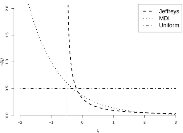
7 (a) Jeffreys (b) MDI (c) Uniform priors for the GP distribution pa-rameters as a function of ξ, withσ = 1. . . 50
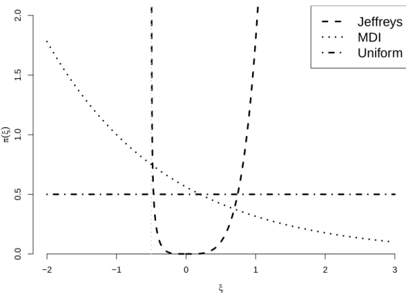
8 (a) Jeffreys (b) MDI (c) Uniform priors for the GEV distribution parameters as a function of ξ, with σ= 1. . . 52
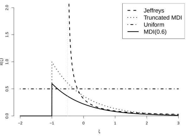
9 (a) Jeffreys (b) truncated MDI (c) generalised truncated MDI(0.6) (d) Uniform priors for the GP distribution parameters as a function of ξ, with σ = 1. . . 61
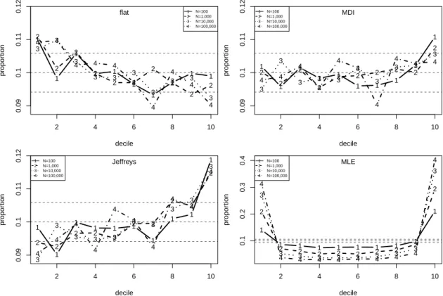
10 Proportions of simulated values ofPb(MN 6x†|xsim) falling in U(0,1) deciles for ξ = 0.1 and pu = 0.5 and for N = 100,1,000,10,000 and 100,000. 95% tolerance limits are superimposed. . . 63
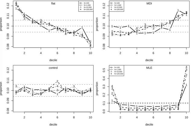
11 Proportions of simulated values ofPb(MN 6x†|xsim) falling in U(0,1) deciles for ξ = 0.1 and pu = 0.1 and for N = 100,1,000,10,000 and 100,000. 95% tolerance limits are superimposed. The control plot is based on random U(0,1) samples. . . 64
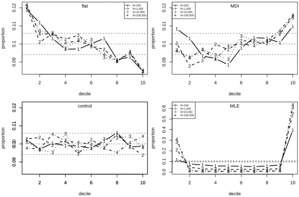
12 Proportions of simulated values ofPb(MN 6x†|xsim) falling in U(0,1) deciles forξ =−0.2 andpu = 0.5 and forN = 100,1,000,10,000 and 100,000. 95% tolerance limits are superimposed. The control plot is based on random U(0,1) samples. . . 65
13 Proportions of simulated values ofPb(MN 6x†|xsim) falling in U(0,1) deciles forξ =−0.2 andpu = 0.1 and forN = 100,1,000,10,000 and 100,000. 95% tolerance limits are superimposed. The control plot is based on random U(0,1) samples. . . 65
14 Proportions of simulated values ofPb(MN 6x†|xsim) falling in U(0,1)
deciles for different combinations of ξ and pu under the truncated
MDI(0.6) prior. Separate lines are drawn forN = 100,1,000,10,000 and 100,000. 95% tolerance limits are superimposed. . . 66 15 Mean residual life plot for Gulf of Mexico storm peak significant wave
height. Dashed lines are the 95% confidence intervals. . . 69 16 Parameter stability plots for Gulf of Mexico storm peak significant
wave height. Vertical lines are the 95% confidence intervals. . . 70 17 Leave-one-out cross-validation for Gulf of Mexico storm peak
signifi-cant wave height. • validation sample ; ◦ training sample. . . 73 18 Leave-one-out cross-validation for Gulf of Mexico storm peak
signifi-cant wave height. • validation sample ;◦ training sample ;− thresh-old excesses. . . 74 19 K-fold cross-validation for Gulf of Mexico storm peak significant wave
height. Blue shaded area forms the validation sample ; Unshaded area forms the training sample. . . 75 20 Repeated random sub-sampling cross-validation for Gulf of Mexico
storm peak significant wave height. • validation sample ; ◦ training sample. . . 76 21 Analysis of Gulf of Mexico significant wave height dataset using an
MDI(0.6) prior for the GP parameters. Estimated threshold weights for validation threshold v, by training threshold u. The upper axis gives the significant wave height scale in metres. . . 85 22 Analysis of Gulf of Mexico significant wave height dataset using an
MDI(0.6) prior, for the GP parameters. N-year predictive return levels and medians of the predictive distribution of MN for N =
100,1,000 and 10,000 by training thresholdu. The upper axis gives the significant wave height scale in metres. . . 87 23 Samples from the posterior distributionπ(σu, ξ|x) using an MDI(0.6)
prior, with superimposed (unnormalised) contours of the posterior density. The dashed lines show the support of the posterior distribu-tion, that is, ξ > σu/(xm −u). A cross shows the posterior mode.
Left: ‘best’ training threshold (based on the 85% and 90% valida-tion thresholds) at 65% sample quantile. Right: 95% sample quantile training threshold. . . 88
upper axis gives the significant wave height scale in metres. . . 89 25 Analysis of North Sea significant wave height dataset using an MDI(0.6)
prior for the GP parameters. Left: estimated threshold weights for validation threshold v, by training threshold u. Right: estimated
N-year predictive return levels and medians of the predictive distri-bution of MN for N = 100,1,000 and 10,000 by training threshold u. The upper axes gives the significant wave height scale in metres. . 90 26 Samples from the posterior distributionπ(σu, ξ|x) using an MDI(0.6)
prior, with superimposed (unnormalised) contours of the posterior density. The dashed lines show the support of the posterior distribu-tion, that is,ξ > σu/(xm−u). A cross shows the posterior mode. Left:
‘best’ training threshold (based on the 85%, 90% and 95% validation thresholds) at 35% sample quantile. Right: 95% sample quantile training threshold. . . 90 27 Predictive medians ofMN compared with the true median (solid black
lines), for datasets simulated from a unit exponential distribution. The set of training thresholds is the 50%,55%, . . . ,95% sample quan-tiles. Grey lines: individual lines for each dataset. Dashed black lines: pointwise 5%, 25%, 50%, 75% and 95% sample quantiles. Threshold strategies: sample median (top left); 95% sample quantile (bottom left); model-averaged estimate (top right); best single threshold (bot-tom right). . . 94 28 Predictive medians ofMN compared with the true median (solid black
lines), for datasets simulated from a standard normal distribution. The set of training thresholds is the 50%,55%, . . . ,95% sample quan-tiles. Grey lines: individual lines for each dataset. Dashed black lines: pointwise 5%, 25%, 50%, 75% and 95% sample quantiles. Threshold strategies: 95% sample quantile (top left); sample median (bottom left); model-averaged estimate (top right); best single threshold (bot-tom right). . . 95
29 Predictive medians ofMN compared with the true median (solid black
lines), for datasets simulated from a hybrid uniform-GP distribution. The set of training thresholds is the 50%,55%, . . . ,95% sample quan-tiles. Grey lines: individual lines for each dataset. Dashed black lines: pointwise 5%, 25%, 50%, 75% and 95% sample quantiles. Threshold strategies: 75% sample quantile (top left); 95% sample quantile (bot-tom left); model-averaged estimate (top right); best single threshold (bottom right). . . 96 30 Summaries of CV weights by training threshold where v = 95%.
Top: the grey lines give individual lines for each simulated dataset with threshold-specific sample means (solid black line) and sample (5, 25, 50, 75, 95)% quantiles (dashed black lines). Bottom: rela-tive frequency with which each threshold has the largest CV weight. Left: exponential distribution. Middle: normal distribution. Right: uniform-GP hybrid distribution. . . 97 31 Summaries of CV weights by training threshold where v = 85%.
Top: the grey lines give individual lines for each simulated dataset with threshold-specific sample means (solid black line) and sample (5, 25, 50, 75, 95)% quantiles (dashed black lines). Bottom: rela-tive frequency with which each threshold has the largest CV weight. Left: exponential distribution. Middle: normal distribution. Right: uniform-GP hybrid distribution. . . 98 32 Model-averaged N-year predictive return levels and selected
quan-tiles of the predictive distribution ofN-year maximumMN, based on
different validation thresholds. Top: Gulf of Mexico data (50% and 85% quantiles of MN). Bottom: North sea data (50%, 75% and 95%
quantiles of MN). . . 99
33 Time series plot of a segment of the Newlyn data illustrating the ‘edges’ (blue shaded area) at the two ends of the observation period. . 103 34 Time series plot of a segment of the Newlyn data illustrating two
examples of validation samples denoted by the blue shaded area (using
v =u= 0.172m andK = 2). Top: Validation sample is the 1st K-gap S1v with value 0. Bottom: Validation sample is the 7thK-gapS7v with value 11. . . 108
gap. The red shaded area denotes the gaps removed from the training sample. . . 110 36 Parameter stability plots for Newlyn sea-surge heights for a range
of run parameter K and using the 60%, 65%, 70% and 75% sample quantile for thresholds. The solid lines give the MLEs of θ and the dashed lines give 95% likelihood-based confidence intervals. . . 112 37 Parameter stability plots for Newlyn sea-surge heights for a range
of run parameter K and using the 80%, 85%, 90% and 95% sample quantile for thresholds. The solid lines give the MLEs of θ and the dashed lines give 95% likelihood-based confidence intervals. . . 113 38 Parameter stability plot for Newlyn sea-surge heights for a range of
thresholds. The solid lines give the MLEs of θ and the dashed lines give 95% likelihood-based confidence intervals. . . 114 39 Threshold selection methods for Newlyn sea-surge heights for a range
of thresholds between the 50%-95% sample quantiles. Top panel: IMT statistic (the red line represents the 5% significance level crit-ical value of 3.84). Bottom panel: threshold weight for validation threshold at 95% sample quantile. . . 115 40 Threshold selection methods for Newlyn sea-surge heights for a range
of thresholds between the 85%-97% sample quantiles. Threshold weights for validation thresholds at 93%, 94%, 95%, 96% and 97% sample quantiles. . . 116 41 Threshold selection for AR(1) process with fixed K = 1. Top panel:
MLE against threshold quantile, with horizontal line at the true value of θ. Middle panel: IMT statistic against threshold quantile, with horizontal line at the critical value for a test with significance level of 5%. Bottom panel: threshold weight against threshold quantile. Each coloured line represents a replication of the simulation. . . 118 42 Threshold selection for AR(2) process with fixed K = 6. Top panel:
MLE against threshold quantile, with horizontal line at the true value of θ. Middle panel: IMT statistic against threshold quantile, with horizontal line at the critical value for a test with significance level of 5%. Bottom panel: threshold weight against threshold quantile. Each coloured line represents a replication of the simulation. . . 120
43 Threshold selection for Markov chain with fixed K = 5. Top panel: MLE against threshold quantile, with horizontal line at the true value of θ. Middle panel: IMT statistic against threshold quantile, with horizontal line at the critical value for a test with significance level of 5%. Bottom panel: threshold weight against threshold quantile. Each coloured line represents a replication of the simulation. . . 121 44 Summaries of threshold weights by training threshold. Top: the grey
lines give individual lines for each simulated dataset with threshold-specific sample means (solid black line) and sample (5, 25, 50, 75, 95)% quantiles (dashed black lines). Bottom: relative frequency with which each threshold has the largest CV weight. Left: AR(1) process. Middle: AR(2) process. Right: MC process. . . 123 45 Summaries of IMT statistics by training threshold. The grey lines
give individual lines for each simulated dataset with threshold-specific sample means (solid black line) and sample (5, 25, 50, 75, 95)% quan-tiles (dashed black lines). The horizontal red line is at the critical value for a test with significance level of 5%. Left: AR(1) process. Middle: AR(2) process. Right: MC process. . . 123 46 Summaries of MLEs by training threshold. The grey lines give
indi-vidual lines for each simulated dataset with threshold-specific sample means (solid black line) and sample (5, 25, 50, 75, 95)% quantiles (dashed black lines). Left: AR(1) process. Middle: AR(2) process. Right: MC process. . . 124 47 Point process representation with varying sample size and with a high
threshold: top left (n = 10), top right (n = 100), bottom left (n = 1000), bottom right (n = 10000). . . 129 48 Point process representation (n= 10000) for different two-dimensional
areas. Plot A: point process according to exceedances above a thresh-old. Plot B: point process according to block maxima. . . 130 49 Non-stationary data (xhas a linear effect on the location of Y) with
a constant threshold (left) and a covariate-dependent threshold (right).136 50 Individual elements ofIM against u1 using symmetric covariate values.141
51 I11and individual elements ofI1 againstu1 using symmetric covariate
values. . . 142
53 Asymptotic standard error of bµ1 againstu1 using asymmetric
covari-ate values. . . 145
List of Tables
1 Tail behaviour for the distribution functionF. . . 23
AR - Autoregressive
ARS - Adaptive Rejection Sampling Bin-GP - Binomial-Generalised Pareto BMA - Bayesian Model Averaging CV - Cross-Validation
ETT - Extremal Types Theorem EVT - Extreme Value Theory FI - Fisher Information
GEV - Generalised Extreme Value GP - Generalised Pareto
i.i.d. - independent and identically distributed IMT - Information Matrix Test
KF - K-Fold
LOO - Leave-One-Out
MC - Markov Chain
MCMC - Markov Chain Monte Carlo MDI - Maximal Data Information MH - Metropolis-Hastings
MLE - Maximum Likelihood Estimation
n.i.d. - non-independent and identically distributed NHPP - Non-Homogeneous Point Process
p.d.f. - probability density function PC - Principal Components POT - Peaks-Over Threshold
PWM - Probability Weighted Moments QR - Quantile Regression
RoU - Ratio of Uniforms
RRSS - Repeated Random Sub-Sampling UETT - Unified Extremal Types Theorem
1 Extreme Value Modelling 19
1
Extreme Value Modelling
Extreme value theory uses asymptotic arguments to suggest models for extreme data. A common practical application of this theory deals with data coming from environmental sources such as rainfall totals, sea wave heights, temperatures etc, when it is of interest to investigate and model the extreme values, in this case the largest values, that these physical phenomena can take.
Thus, the main goal of extreme value modelling is to enable extrapolation, i.e. to infer the stochastic behaviour of a quantity at levels beyond those already observed. A specific example of the practical use of extreme value modelling can be found in marine engineering. The design of marine structures, such as oil platforms, requires information about the most extreme sea conditions likely to be encountered over some future long time period, for example 100, 1000 or even 10,000 years. A common variable used for this purpose is the significant wave height. One can use extreme value theory to suggest models for large significant wave heights, such as the largest value observed over a period of one year or the amounts by which a high threshold is exceeded.
In this chapter we introduce the models involved in extreme value theory. More specifically in section 1.1 we consider the simplest case: univariate independent and identically distributed (i.i.d.) sequences and introduce the two main models, namely, the Generalised Extreme Value (GEV) model (for block maxima) and the Gener-alised Pareto (GP) model (for threshold excesses). Later in section 1.6 we consider the case for univariate dependent sequences and introduce the K-gaps exponential mixture model (for threshold inter-exceedance times). The theory outlined in this chapter is a summary of fundamental results that are central to this research. We also provide a number of relevant references where the reader can find more details about these results and demonstrate the methodology through simple examples and graphical illustrations. Finally, we conclude this chapter with an outline of the thesis and the topics covered in the remaining chapters.
1.1
Extreme Value Theory for univariate independent
se-quences
Let us assume that we have a sequence of independent random variablesX1, . . . , Xm
with an identical but unknown distribution function F. Often {Xi} is a
discrete-time process observed on regular discrete-time intervals, such as days. The starting point of extreme value theory is to consider the statistical behaviour of the block maximum
Mn = max{X1, . . . , Xn}, for a block size n6m, as n→ ∞.
Under the assumed independence of the Xis the distribution function of Mn is
derived as
P(Mn 6x) = P(X1 6x, . . . , Xn 6x)
= P(X1 6x)× · · · ×P(Xn6x)
= {F (x)}n.
Since the distribution function F is unknown, we investigate the behaviour of
{F (x)}n as the block sizenincreases. The main concern is the fact that the asymp-totic distribution of Mn degenerates to a point mass as Mn converges to the upper
endpoint, xF = sup{x:F(x)<1}, of F, that is, for any value ofx
lim n→∞{F (x)} n = 1 if F(x) = 1, 0 if F(x)<1.
The standard approach to steer clear from this problem is to seek a linear normal-ization
Mn∗ = Mn−bn
an
of Mn, where an > 0 and bn are sequences of constants, so that as n → ∞ a
non-degenerate limiting distribution results for Mn∗.
The question of importance is “what kinds of limiting distribution for Mn∗ are pos-sible”?
1.1.1 Extremal Types Theorem (ETT)
Fisher and Tippett (1928) were the first to describe the asymptotic properties of the normalised block maximum from an unknown distribution function F. The work by Gnedenko (1943) completed in generality this important result, known as
the Extremal Types Theorem. A detailed proof of this theorem can be found in
Leadbetter et al. (1983).
Theorem 1. Extremal Types Theorem (ETT).
If there exist sequences of constants an >0 and bn such that
P Mn−bn an 6 x →G(x), as n→ ∞,
1.2 Generalised Extreme Value (GEV) distribution 21
where G is a non-degenerate distribution function, then G will belong to one of the
following distribution families:
Gumbel: G(x) = exp −exp − x−b a , −∞< x < ∞; Fr´echet: G(x) = 0, x6b, exp ( − x−b a −k) , x > b, k >0; Weibull: G(x) = exp ( − " − x−b a k#) , x < b, k >0, 1, x>b,
for some location parameter b, scale parameter a >0 and shape parameter k.
Fisher and Tippett (1928) showed that in fact these three distribution families are the only possible limit distributions for the block maximum irrespective of the un-known distribution F of the population. If, for a given F, the Gumbel limit is obtained, we say thatF is in the domain of attractionof the Gumbel extreme value family, and similarly for the Fr´echet and Weibull families.
Historically, when extreme value theory was used to analyse a dataset, a subjective decision was taken a priori as to which of the three families applied. This was a necessary part of the process that was followed by an estimation of the parame-ters of the distribution that was chosen. However, since each family describes the tail behaviour of the distribution differently there were clear drawbacks with this method:
• it introduced the argument of how the distribution choice should be made;
• it did not allow for uncertainty about the correct distributional choice. These problems are overcome by combining the three limiting forms into a single family.
1.2
Generalised Extreme Value (GEV) distribution
The Generalised Extreme Value (GEV) distribution was derived by Jenkinson (1955) and von Mises (1964), which uses a parameterisation to integrate the three different distribution families into one. Therefore we can restate theorem 1 as theorem 2.
Theorem 2. Unified Extremal Types Theorem (UETT).
If there exist sequences of constants an >0 and bn such that
P Mn−bn an 6 x →G(x), as n→ ∞,
where G is a non-degenerate distribution function, then G is a GEV distribution
function G(x) = exp ( − 1 +ξ x−µ σ −1/ξ + ) , (1.1)
for parameters −∞< µ <∞, σ >0 and −∞< ξ <∞, where a+ = max(a,0).
Thus, the GEV(µ, σ, ξ) distribution (with location parameter µ, scale parameter
σ and shape parameter ξ) is defined on {x: 1 +ξ(x−µ)/σ >0}. The Gumbel distribution is obtained in the limit as ξ→0.
1.2.1 Max Stability
An informal proof of theorem 2 centres on the concept of max-stability. Firstly we note that two distributions are of the same type if they differ only in their location and/or scale parameters. A distribution G is said to be max-stable if there are constants an>0 and bn such that for everyk = 2,3. . .,
Gk(anx+bn) = G(x),
that is, taking block maxima from a distribution functionGresults in a distribution of the same type of the original distribution G.
It makes sense that if a limiting distribution function G for linearly normalised maxima exists then G must be max-stable: if Mn∗ has approximate distribution function G, thenMnk∗ , k>1, should have a distribution function of the same type, otherwise convergence has not yet been achieved. In fact, Leadbetter et al. (1983) show that the only distribution that is max-stable is the GEV.
1.2.2 Tail behaviour
In practice we assume tentatively that (a) the F from which the data are produced is in the domain of attraction of the GEV family and (b) the value of n is large enough that a GEV distribution is good approximation to the distribution of Mn.
1.2 Generalised Extreme Value (GEV) distribution 23
This motivates the use of a GEV distribution as a model to the maxima of large numbers of i.i.d. random variables. In practice F is unknown, so the normalising constants an and bn are also unknown. However, this is not a problem because an
and bn appear in the location and scale of the distribution of Mn and are to be
estimated anyway. We discuss statistical inference for extreme value models later in section 1.5.
The important benefit of using the GEV model for extreme data analysis, as com-pared to the historical approach that was described earlier is the fact that it does not need a prior subjective choice of an extreme value family to which the data belong.
The following table summarises informally the tail behaviour of the distribution according to the value of ξ. The value of ξ determines which of the historical extreme value family applies and whether the upper endpointxF is finite (ξ <0) or
infinite (ξ >0).
ξ Tail behaviour Distribution Family
ξ = 0 Exponential upper tail Gumbel
ξ >0 Heavy upper tail Fr´echet
ξ <0 Finite upper limit Weibull
Table 1: Tail behaviour for the distribution function F.
1.2.3 Domains of attractions
It is of theoretical interest to consider what properties F must have to be in the domain of attraction of a particular extreme value distribution. Leadbetter et al. (1983) state in section 1.6 the necessary and sufficient conditions for this. They show proves for the sufficiency and provide references for the proves of the neces-sity. However, for simplicity, here we follow Smith (1987) and restrict attention to absolutely continuous distribution functions F.
We begin with the hazard function h(x) which can be thought of loosely as the instantaneous probability that X =x given that X > x. We define the reciprocal hazard function η(x) = 1/h(x) by
η(x) = 1−F(x)
f(x) , xF < x < x
F ,
distribution and f(x) is the probability density function.
Studying the behaviour of the (reciprocal) hazard function for large xindicates how heavy is the upper tail of F. For example, if F is the distribution function of an exponential random variable, then η(x) is constant for all x. In contrast, heavy (light) upper tails produce η(x) that increase (decrease) as x →xF. Therefore the derivative η0(x) = dη(x)/dxof η(x) is key.
If η0(x) tends to a finite limit ξ as x → xF (the von Mises’ condition) then F is
in the domain of attraction of a GEV distribution with shape parameter ξ. Thus the limiting distribution of Mn is determined by the upper tail of F. Also, suitable
normalising constants are given bybn =F−1(1−1/n) andan=η(bn). These results
are not of practical use unless we have some knowledge about the tail behaviour of
F.
1.3
Generalised Pareto (GP) distribution
The results in section 1.2 relate to block maxima, i.e. the largest ofnvalues. One can argue that since other values in each block are not utilised this method is somewhat wasteful and potentially important information might be lost. A better approach is to use an alternative definition of an extreme value, namely, that an observation is extreme if it exceeds some high threshold u.
Let us assume again that we have a sequence of independent, identically distributed random variables X1, . . . , Xm with a distribution function F which is unknown.
We introduce a threshold denoted by u. We describe in more detail the various approaches of how an appropriate value of u can be chosen in chapter 3.
Threshold modelling of extremes is based on two aspects: (i) the probabilitypu that
the threshold uis exceeded, and (ii) the amount by which the threshold is exceeded when it is exceeded. We use the terminologyexceedanceto refer to anXthat exceeds
u and define the corresponding thresholdexcess byZ = (X−u)|X > u. Theorem 3 motivates the use of a particular distribution to model the threshold excess Z. Theorem 3. Limiting distribution of threshold excesses.
If theorem 2 holds then as u→ ∞, the distribution function of (X−u) |X > u is
approximately H(z) = 1− 1 + ξz σu −1/ξ + , z >0, (1.2) where σu =σ+ξ(u−µ).
1.4 Gulf of Mexico data 25
This is the distribution function of a Generalised Pareto (GP) distribution (Pickands, 1975) defined on 0 < z < −σu/ξ if ξ < 0 and z > 0 if ξ > 0 and characterised by
a scale parameter σu satisfying σu > 0 and a shape parameter ξ satisfying −∞ < ξ < ∞. An exponential distribution with rate parameter 1/σu is obtained in the
limit as ξ→0. This result motivates the use of the GP(σu, ξ) distribution to model
excesses of a high threshold u. In common with the GEV distribution, the shape parameter value determines whether or not xF is finite as in table 1. Coles (2001, pages 76-77) gives an informal justification of theorem 3 with a more formal proof provided by Leadbetter et al. (1983).
1.3.1 Binomial-Generalised Pareto (Bin-GP) model
This theory motivates the Binomial-Generalised Pareto (Bin-GP) model with pa-rameters (pu, σu, ξ). Under the assumed independence of X1, . . . , Xm the number of
exceedances of the threshold u(denoted by nu) has a Bin(m, pu) distribution.
The Bin-GP model’s parameters are related to the GEV parameters (µ, σ, ξ) via
σu =σ+ξ(u−µ) and pu = 1−F(u)≈ 1 n 1 +ξ u−µ σ −1/ξ ,
where m is the complete length of the data set, n is the block size that is used to define Mn and the approximate expression for pu follows from Coles (2001, pages
76-77).
1.4
Gulf of Mexico data
In this section we briefly describe a motivating example of how extreme value anal-ysis can be applied in a practical situation using the GEV and GP distributions. Firstly we introduce the dataset that is used for these analyses.
The data come from Oceanweather’s metocean study for the Gulf of Mexico called GOMOS (Oceanweather Inc., 2005). They are hindcasts of a conventional measure of sea surface roughness, significant wave height (Hs), defined as the mean of the
highest one third of wave heights. The hindcasts are produced by a physical model, calibrated to observed hurricane data, resulting in Hs values on a spatial grid
ev-ery 30 minutes between September 1900 to September 2005. The motivation for analysing these data comes from marine engineering and more specifically the at-tempt to develop some design criteria for marine structures, such as oil platforms, where it is of great value to understand better the stochastic behaviour of extreme
weather events, such as the hurricanes that occur in the Gulf of Mexico.
Hurricanes are clearly-defined events, so it is straightforward to isolate from raw time series the largest Hs value, the storm peak significant wave height Hssp, for
each hurricane event. This eliminates within-event temporal dependence so that
Hssp values from different events can be treated as being independent. The full dataset, which has been analysed by Jonathan and Ewans (2007, 2011), Northrop and Jonathan (2011), consists of hindcastHsp
s values for a 6×12 grid of 72 sites in
an unnamed location in the Gulf of Mexico. Here we consider a single site (site 31) at the centre of the grid. The data are displayed in figure 1.
● ● ●● ● ● ● ● ● ● ● ● ● ● ● ● ● ● ● ● ● ● ● ● ● ● ● ● ● ● ● ● ● ● ● ●● ●● ● ● ● ● ● ● ● ● ●● ● ● ● ● ● ● ● ● ● ● ● ● ● ● ● ●● ● ● ● ● ● ●● ● ● ●● ● ●●● ● ● ● ● ● ● ● ● ● ● ● ● ● ● ●● ● ● ● ● ●● ● ● ● ● ● ● ● ● ● ● ● ● ● ● ● ●● ● ● ● ● ● ● ● ● ● ●● ● ● ● ● ● ● ● ● ● ● ●● ● ● ● ● ● ● ● ● ● ● ● ● ● ● ● ● ● ● ● ● ● ● ● ● ● ● ●● ● ●● ● ● ● ● ● ● ● ●● ● ● ● ● ● ● ● ● ● ● ● ● ● ● ●● ●● ●● ● ●● ● ● ● ● ● ● ● ● ● ●● ● ● ● ● ● ●● ● ● ● ● ● ● ● ● ● ● ● ●●● ● ● ● ● ● ● ● ● ● ● ●●● ● ● ● ● ● ● ●● ● ● ● ● ● ● ● ● ● ● ● ● ● ● ● ● ● ● ● ● ● ● ● ● ● ● ● ● ● ● ● ● ● ● ● ● ● ● ●● ● ● ● ● ● ● ● ● ● ●● ● ● ● ● ● 1900 1920 1940 1960 1980 2000 0 5 10 15 Year Stor m peak significant w a v e height (m)
Figure 1: Time series plot of Gulf of Mexico storm peak significant wave heights.
1.4.1 GEV - Block Maxima approach
The first method of extreme value analysis that we describe here is known as the
block maxima approach. This involves dividing the data into blocks of equal length
and then fitting a GEV distribution to the block maxima. A typical choice in environmental applications is a block size equating to one year of observations, which produces annual maxima. It is important to note that the decision about the block size leads to a trade-off between bias and variance. On one hand, deciding on a small block size might violate the asymptotic arguments for the limiting GEV
1.4 Gulf of Mexico data 27
distribution leading to bias. On the other hand, a large block size will provide few points (block maxima) to use for statistical inference and this can result in parameter estimators with high variances. Figure 2 illustrates the blocking procedure using the Gulf of Mexico data.
● ● ●● ● ● ● ● ● ● ● ● ● ● ● ● ● ● ● ● ● ● ● ● ● ● ● ● ● ● ● ● ● ● ● ●● ●● ● ● ● ● ● ● ● ● ●● ● ● ● ● ● ● ● ● ● ● ● ● ● ● ● ●● ● ● ● ● ● ●● ● ● ●● ● ●●●● ● ● ● ● ● ● ● ● ● ● ● ● ● ●● ● ● ● ● ●● ● ● ● ● ● ● ● ● ● ● ● ● ● ● ● ●● ● ● ● ● ● ● ● ● ● ●● ● ● ● ● ● ● ● ● ● ● ●● ● ● ● ● ● ● ● ● ● ● ● ● ● ● ● ● ● ● ● ● ● ● ● ● ● ● ●● ● ●● ● ● ● ● ● ● ● ●● ● ● ● ● ● ● ● ● ● ● ● ● ● ● ●● ●● ●● ● ●● ● ● ● ● ● ● ● ● ● ●● ● ● ● ● ● ●● ● ● ● ● ● ● ● ● ● ● ● ●●● ● ● ● ● ● ● ● ● ● ● ●●● ● ● ● ● ● ● ●● ● ● ● ● ● ● ● ● ● ● ● ● ● ● ● ● ● ● ● ● ● ● ● ● ● ● ● ● ● ● ● ● ● ● ● ● ● ● ●● ● ● ● ● ● ● ● ● ● ●● ● ● ● ● ● 1900 1920 1940 1960 1980 2000 0 5 10 15 Year Stor m peak significant w a v e height (m) ● ● ● ● ● ● ● ● ● ● ● ● ● ● ● ● block maxima
Figure 2: Identification of block maxima.
As this plot is merely illustrative, 15 blocks of 7 years were chosen for convenience. We then treat the block maxima as a random sample from a GEV(µ, σ, ξ) distribu-tion.
1.4.2 GP - Threshold exceedances approach
As an alternative to the block maxima approach, let us assume that a high threshold
u is chosen for this dataset. If an observation is higher then u, then this is an exceedance ofuand the amount by which the observation exceeds uis the threshold excess. Appealing to theorem 3 suggests the GP distribution as a model for the threshold excesses. This is illustrated in figure 3 below.
● ● ●● ● ● ● ● ● ● ● ● ● ● ● ● ● ● ● ● ● ● ● ● ● ● ● ● ● ● ● ● ● ● ● ●● ●● ● ● ● ● ● ● ● ● ●● ● ● ● ● ● ● ● ● ● ● ● ● ● ● ● ●● ● ● ● ● ● ●● ● ● ●● ● ●●●● ● ● ● ● ● ● ● ● ● ● ● ● ● ●● ● ● ● ● ●● ● ● ● ● ● ● ● ● ● ● ● ● ● ● ● ●● ● ● ● ● ● ● ● ● ● ●● ● ● ● ● ● ● ● ● ● ● ●● ● ● ● ● ● ● ● ● ● ● ● ● ● ● ● ● ● ● ● ● ● ● ● ● ● ● ●● ● ●● ● ● ● ● ● ● ● ●● ● ● ● ● ● ● ● ● ● ● ● ● ● ● ●● ●● ●● ● ●● ● ● ● ● ● ● ● ● ● ●● ● ● ● ● ● ●● ● ● ● ● ● ● ● ● ● ● ● ●●● ● ● ● ● ● ● ● ● ● ● ●●● ● ● ● ● ● ● ●● ● ● ● ● ● ● ● ● ● ● ● ● ● ● ● ● ● ● ● ● ● ● ● ● ● ● ● ● ● ● ● ● ● ● ● ● ● ● ●● ● ● ● ● ● ● ● ● ● ●● ● ● ● ● ● 1900 1920 1940 1960 1980 2000 0 5 10 15 Year Stor m peak significant w a v e height (m) ● ● ● ● ● ● ● ● ● ● ● ● ● ● ● ● u ● exceedances of u excesses of u
Figure 3: Threshold exceedances and excesses of u.
Here, we have applied a threshold of 7.0798m which corresponds to the 95th quan-tile of the data. We treat these excesses as a random sample from a GP(σu, ξ)
1.4 Gulf of Mexico data 29 ● ● ●● ● ● ● ● ● ● ● ● ● ● ● ● ● ● ● ● ● ● ● ● ● ● ● ● ● ● ● ● ● ● ● ●● ●● ● ● ● ● ● ● ● ● ●● ● ● ● ● ● ● ● ● ● ● ● ● ● ● ● ●● ● ● ● ● ● ●● ● ● ●● ● ●●●● ● ● ● ● ● ● ● ● ● ● ● ● ● ●● ● ● ● ● ●● ● ● ● ● ● ● ● ● ● ● ● ● ● ● ● ●● ● ● ● ● ● ● ● ● ● ●● ● ● ● ● ● ● ● ● ● ● ●● ● ● ● ● ● ● ● ● ● ● ● ● ● ● ● ● ● ● ● ● ● ● ● ● ● ● ●● ● ●● ● ● ● ● ● ● ● ●● ● ● ● ● ● ● ● ● ● ● ● ● ● ● ●● ●● ●● ● ●● ● ● ● ● ● ● ● ● ● ●● ● ● ● ● ● ●● ● ● ● ● ● ● ● ● ● ● ● ●●● ● ● ● ● ● ● ● ● ● ● ●●● ● ● ● ● ● ● ●● ● ● ● ● ● ● ● ● ● ● ● ● ● ● ● ● ● ● ● ● ● ● ● ● ● ● ● ● ● ● ● ● ● ● ● ● ● ● ●● ● ● ● ● ● ● ● ● ● ●● ● ● ● ● ● 1900 1920 1940 1960 1980 2000 0 5 10 15 Year Stor m peak significant w a v e height (m) ● ● ● ● ● ● ● ● ● ● ● ● ● ● ● ● ● ● ● ● ● ● ● ● ● ● ● ● ● ● ● u ● ● exceedances of u block maxima
Figure 4: Comparison of block maxima and threshold exceedances.
Figure 4 above illustrates the ‘extreme’ points through both of the described ap-proaches and shows some important features: (i) that some of the block maxima (shown in blue) are not included in the threshold modelling approach of extreme value analysis, (ii) some second (and third and fourth) largest values in a block are included in the threshold approach and (iii) there are very few exceedances above the threshold from which the inferences about the GP(σu, ξ) distribution will be
made.
The third point could be addressed by choosing a lower threshold, which will result in more threshold exceedances. However, the solution is not that straightforward because, similarly to the block maxima approach, a bias-variance trade-off is also present in the threshold modelling approach. Choosing too low a threshold leads to bias due to the GP model being inappropriate and too high a threshold results in a small number of exceedances and unnecessarily low estimation precision. We develop new methods for addressing this bias-variance trade-off for a independent and identically distributed stationary process in chapter 3 and for a dependent and identically distributed stationary process in chapter 4.
1.5
Statistical modelling and parameter estimation
One of the tasks that a statistician needs to tackle when having a dataset is to analyse the data and make inferences about the parameters of the supposed random process that generated this data. More specifically, if we are interested in analysing extreme values from a data source, we need to be able to say something about an assumed model and its parameters. By doing so, we can better understand and describe the process and more importantly make inferences on the stochastic behaviour of more extreme observations.
In this section we outline methods of inferences used commonly in extreme value modelling. We concentrate on likelihood-based methods as they can, in principle, be used in a wider variety of modelling situations than competing methods. In particular, they apply more generally than in the simple i.i.d. case we consider initially.
Likelihood and log-likelihood functions
Let us assume that we have a sequence of independent and identically distributed random variables X1, . . . , Xm with probability density function f(xi;θ), where the
stochastic process of the observed data is characterized by the vectorθ, ak-dimensional set of parameters. The joint density of the random variables is defined as the likeli-hood function L(θ;x1, . . . , xm) = m Y i=1 f(xi;θ) for i= 1, . . . , m, (1.3)
which is a function defined by the set of unknown parameter vector θ.
Using the fact that the natural logarithm function is monotonic, it is more convenient to work with the log-likelihood function
`(θ;x1, . . . , xm) = logL(θ;x1, . . . , xm) = m
X
i=1
logf(xi;θ). (1.4)
Score Function and Fisher Information
Thescore functionis defined as the vector (of lengthk) of the first partial derivatives
of the log-likelihood function
S(θ;X1, . . . , Xm) = ∂
1.5 Statistical modelling and parameter estimation 31
The score function is itself a vector of random variables and has the following sta-tistical properties. The mean of the score, evaluated at the true set of parametersθ is found to be zero and its variance is a symmetric k×k variance-covariance matrix which is called the (expected) Fisher Information matrix (FI)and is defined as
I(θ) =E " ∂ ∂θ`(θ;X1, . . . , Xm) 2# .
Due to the assumed independence and under some regularity conditions the F I
matrix can also be written as
F I =I(θ) = −E ∂2 ∂θ∂θT`(θ;X1, . . . , Xm) .
We usually estimate I(θ) by the observed Fisher information
J(θ) = − ∂2
∂θ∂θ`(θ;x1, . . . , xm). If the stochastic process of the observed data is characterized by the vector θ of length k, then matrix F I as defined above will be a k×k positive semi-definite symmetric matrix.
1.5.1 Maximum Likelihood Estimation
A widely used and flexible approach for parameter estimation is maximum likelihood. The aim of this approach is to obtain the set of parameter estimates for which the joint probability density of the observed data is maximised. In practice, the log-likelihood (1.4) is maximised with respect to θ to obtain the maximum likelihood estimate (MLE) θ.b
On the condition that the log-likelihood is concave, setting the score function
S(θ;X1, . . . , Xm) to zero and solving for θ will result to the vector of maximum
likelihood estimators, θ. Furthermore, in regular estimation problems, for a largeb
sample size m it can be shown that, approximately
b
θ ∼N(θ,I(θ)−1). (1.5)
Expressions for the log-likelihood and the Fisher information based on a random sample from a GEV distribution are given in A.1. A.2 gives these expressions for the GP case.
Regularity conditions
an estimation problem needs to satisfy in order for maximum likelihood estimation to
beregular. One regularity condition is that the support of the distribution does not
depend on the parameter values. This however, is not the case for either the GEV or GP distribution, so estimating the parameters of these models using maximum likelihood is not automatically a regular estimation problem.
Smith (1985) carried out a theoretical analysis to examine the regularity conditions that are necessary for the estimation to be regular. In cases like the GEV and GP distributions Smith (1985) shows that if ξ > −1/2 then maximum likelihood estimation is regular and the resulting maximum likelihood estimator has the usual properties such as (1.5). The reason that this estimation problem is irregular for
ξ 6−1/2 is that the variance of the score function, var[S(θ;X1, . . . , Xm)], does not
exist unless ξ > −1/2. Smith (1994) extends this result to the regression situation to show that a covariate dependent shape parameter would still need to be greater than −1/2 for all values of the covariates.
1.5.2 Bayesian Inference
Let us assume that we have a vector of data x = (x1, . . . , xm) from a sequence
of i.i.d. random variables. For example x could represent hindcast storm peak significant wave heights,Hsp
s as introduced in 1.4. In maximum likelihood estimation
(afrequentistmethod of inference), the parameter vectorθ is viewed as a unknown,
but fixed, value to be estimated. In Bayesian inference θ is viewed as a random variable. A prior distribution π(θ), representing uncertainty about θ external to the data x, is specified. Prior information about θ, contained in π(θ), is combined with information from the data, contained in the likelihood L(x;θ), using Bayes’ theorem. This results in a posterior distribution π(θ | x) that is proportional to
L(x;θ)π(θ) as
π(θ|x)∝π(θ)×L(x;θ), (1.6)
where the normalising constant is 1/RΘπ(θ)L(x;θ) dθ. Subject to the assumptions made, the posterior distribution gives the distribution of the model parameters conditional on the data observed.
The advantages of a Bayesian analysis (over maximum likelihood estimation) in an extreme value context are:
(a) the ξ >−1/2 regularity condition is not required; (b) information external to the data can be incorporated;
1.5 Statistical modelling and parameter estimation 33
(c) predictive inference, in which predictions of future extreme events account ap-propriately for model parameter uncertainty, is handled naturally.
Points (b) and (c) are particularly relevant because, by their nature, samples of suit-ably extreme data can be small. This often results in large uncertainty about model parameters and consequently about extrapolation in the future. Use of prior infor-mation can alleviate this problem. Moreover, sample sizes are often small enough that maximum likelihood estimators are far from normally distributed. This means that a frequentist approximation to predictive inference based on normality can be misleading.
In chapters 3 and 4 it is important that we can perform predictive inference reliably, so we take a Bayesian approach. This requires a prior distribution to be specified. In the absence of genuine prior information, the question arises: “Which prior should we use?”. We consider this question in chapter 2.
1.5.3 Other methods of inference
There are many methods of inference that have been used in extreme value modelling (see for example Beirlant et al. (2004, Chapter 5), Kotz and Nadarajah (2000), Coles (2001)). Here we briefly describe another popular inference method, namely, the Probability Weighted Moments (PWM), that is often used as an alternative to MLE. This method has been historically used to estimate the parameters of the GEV (Hosking et al., 1985) and the GP (Hosking and Wallis, 1987) distributions and is particularly popular in hydrology and climatology.
Greenwood et al. (1979) introduce the general PWM method which is as follows. For a sequence of i.i.d. random variables X1, . . . , Xm with distribution function F(x),
the PWM can be found by evaluating
E[Xp(F(X))r(1−F(X))s], (1.7) where p,r and s are real numbers.
In the case of extreme value modelling, the PWM method for obtaining model parameter estimators is limited, similarly to the MLE, to parameter space of the shape parameter. More specifically Hosking et al. (1985) showed that the asymptotic properties of the PWM estimators exist only when ξ <0.5.
Many authors have compared MLE and PWM, including Landwehr et al. (1979), Hosking et al. (1985), Hosking and Wallis (1987), Coles and Dixon (1999), Martins
and Stedinger (2000) to name a few. In particular it was found that PWM can perform better for small sample sizes, with the PWM estimators having smaller variance. However, Coles and Dixon (1999) note that the smaller variance of the PWM estimators is partly achieved in place of higher bias as compared to the MLE method due to the parameter space restriction in PWM. Furthermore, it is worth pointing out that the PWM method does not extend easily beyond the i.i.d. case.
1.6
Extreme Value Theory for univariate dependent sequences
So far we have introduced the relevant background theory involving observations from univariate sequences of i.i.d. random variables. In this section we relax the independence property and briefly describe the theory behind non-independent and identically distributed (n.i.d.) random variables, i.e. a stationary sequence of ran-dom variables whose joint distribution does not change over time.
It is reasonable to accept, especially in environmental data, that an extreme event can be followed closely by another extreme event and that the assumption of inde-pendence is questionable. In fact, it is very common for extreme observations to occur in clusters. The properties of dependent extremes are analysed in detail in Leadbetter et al. (1983, Chapter 3). Chavez-Demoulin and Davison (2012) provide a review of the modelling of the extremes of dependent sequences. We first look at the theory behind block maxima and later concentrate on threshold-based models. It is not possible to develop a theory for the extremes of dependent sequences that is akin to the UETT of theorem 2, unless some constraint is placed on the form of tem-poral dependence in the sequence. For example, in the extreme case of perfect depen-dence, i.e. Xt =X1, for t = 1,2, . . ., the distribution function of max(X1, . . . , Xn)
is identical to that of X1 (F say) for all n. Therefore, the limiting distribution
function ofMn isF, which could be anything. However, to make progress it is only
necessary to place a constraint on the strength of long-range dependence at extreme levels: that occurrences of extreme events are approximately independent provided that these events are sufficiently separated in time. More specifically, a sufficient constraint is the following D(un) condition (Leadbetter et al., 1983, section 3.2).
Condition D(un)
Let X1, X2, . . . be a stationary sequence of random variables. The sequence satisfies
the D(un) condition, if for all i1 <· · ·< ip < j1 <· · ·< jq with j1−ip > l,
1.6 Extreme Value Theory for univariate dependent sequences 35
where A is the event that Xi1 6 un, . . . , Xip 6 un, B is the event that Xj1 6
un. . . , Xjq 6un, there exists a sequence ln such that ln/n→0 as n→ ∞ for which
α(n, ln)→0 as n → ∞.
This is a weak condition (the form of short-term dependence is not restricted) and is plausible for many physical processes. The UETT extends to stationary sequences that satisfy this condition, but the strength of short-term dependence in the extremes of the sequence has an effect on the location, and perhaps the scale, of the limiting GEV distribution, in a way that the following theorem, found in Leadbetter et al. (1983, section 3.3), makes precise.
Theorem 4. Extremes of dependent sequences.
Let X1, X2, . . . be a sequence of independent random variables with marginal
dis-tribution function F and let X1e ,X2e . . . be a stationary sequence of dependent
ran-dom variables satisfying D(un) condition, with the same marginal distribution
func-tion. Let Mn = max{X1, . . . , Xn} and Mfn = max
n e
X1, . . . ,Xen
o
. If, as n → ∞,
P({(Mn−bn)/an6x} →G(x), for normalising sequences an>0 and bn, then
P n(Mfn−bn)/an 6x
o
→Gθ(x) (1.8)
for some 0< θ61.
The max-stability of G means that Gθ is a GEV distribution function. Therefore,
this theory suggests the GEV distribution as a model for block maxima, as in the independent case.
1.6.1 Extremal index
The quantity θ is known as the extremal index. It is the most common measure of the strength of short-term (local) temporal dependence in extremal behaviour. The closer θ is to zero the stronger is the local dependence at extreme levels. For a sequence with θ = 1 there is no local dependence asymptotically but there may be dependence at levels of practical interest.
The extremal index is involved in several characterisations of local extremal depen-dence based on the extent to which exceedances of a suitably high threshold occur in clusters. Asymptotically (in a sense that we make more precise in section 1.7) the mean number of exceedances in a cluster is given by 1/θ and suitably rescaled times between the last exceedance of one cluster and the first exceedance of the next cluster are exponentially distributed with mean 1/θ.
The extremal index is important because it affects extremal inferences. Theorem 4 implies that for large n, P(Mfn 6 x) ≈ Gθ(x) = F(x)nθ. If we wish to infer
from an estimate of F the distribution of the largest value to be observed over some future long time interval then the value of θ matters. Ignoring clustering would lead to overestimation of quantiles of Mn. The extremal index also affects
interpretation of extremal inferences because it determines the way in which extreme events (exceedances of some high threshold) occur. Consider two cases, each with the same F. If θ = 1 then threshold exceedances occur singly at some rate λ, say, in time. If θ = 1/10 then threshold exceedances occur in clusters of mean size 10 at a smaller rate λ/10, i.e. exceedances tend to occur together but there is a larger probability of seeing no such cluster in a given period of time. The difference in behaviour may be important practically.
The presence of local dependence also complicates statistical inference and the se-lection of an appropriate threshold. Reliable estimation of θ is crucial and many methods have been proposed for achieving this. Of the threshold-based methods we concentrate on those proposed by Ferro and Segers (2003), S¨uveges (2007) and S¨uveges and Davison (2010). In section 1.7 we describe the theory underlying these methods and in chapter 4 we use the model proposed by S¨uveges and Davison (2010) to perform threshold selection. In the next section we outline different general ap-proaches to threshold modelling of serially-dependent extremes.
1.6.2 Threshold-based statistical inference
The presence of local extremal dependence makes threshold-based inferences more difficult than in the independent case. Ifθ <1 then there will be some clustering of exceedances at all levels and one cannot eliminate the potential problem of within-cluster dependence between exceedances by setting a high threshold. Although asymptotic theory suggests a GP distribution as a marginal model for (all) threshold excesses it is not appropriate to treat these excesses as independent.
One way round this problem is to extract from the data a set of threshold excesses that can be treated as approximately independent. This is achieved by specify-ing a rule to identify clusters of exceedances, a procedure known as declustering. Exceedances greater than a certain number of observations (the run length) apart are deemed to be in different clusters, otherwise they are put in the same cluster. Ferro and Segers (2003) automate this process by basing the run length on an es-timate of θ. From each cluster the largest excess is extracted, producing a sample of cluster maxima. Then a GP distribution is fitted to these cluster maxima, the
1.7 K-Gaps exponential mixture model 37
However, Fawcett and Walshaw (2007) demonstrate that, in addition to the loss of statistical precision that results from using only cluster maxima, the declustering process leads to serious bias. They show that it is better to base inferences on all
threshold excesses: point estimates are based on a likelihood in which the excesses are assumed to be independent, but estimates of parameter uncertainty are adjusted to account for the dependence between these excesses. Fawcett and Walshaw (2012) update this work to incorporate uncertainty aboutθin extreme value extrapolations. An alternative approach is to model within-cluster dependence explicitly (Smith et al., 1997, Fawcett and Walshaw, 2006). This is essential in applications where it is important to gain insight about the nature of this dependence. A common approach is to specify a first-order Markov chain for threshold excesses, based on a particular bivariate extreme value model. However, this raises the issue of which member of the wide class of such models to use. Otherwise, i.e. if it is only necessary to adjust inferences for the strength of local dependence as summarised by θ, then the approach of Fawcett and Walshaw (2012) may be preferable.
It is common to ignore local dependence in extremes at the threshold selection stage, although such dependence can be expected to have an impact. An informal way to include the impact of threshold in terms of local dependence is to choose a threshold above which estimates of the extremal index θ are judged to be insensitive to the threshold. However, in practice estimates ofθoften do not stabilise in a clear way as the threshold increases, making this judgement difficult. A more formal model-based approach is developed by S¨uveges and Davison (2010). In chapter 4 we propose an alternative approach based on the same underlying model, which we describe in the next section.
1.7
K-Gaps exponential mixture model
Let us assume that we have a stationary processXe1,Xe2, . . . ,with unknown marginal
distribution function F. The following theorem is given by S¨uveges and Davison (2010, page 206). For a sequence of thresholds un, introduce the random variable
T(un) = min{k >1 :Xek+1 > un|Xe1 > un},
for the inter-exceedance times in the sequence {Xei} and the corresponding K-gaps
random variable by
Let Fi,j(un) denote the σ-field (Billingsley, 1995, pages 20-21) generated by the
events Xer 6 un, r = i, . . . , j. In simple terms, Fi,j(un) defines the possible
combi-nations of the events Xer 6 un, r = i, . . . , j that can be assigned probabilities. For
any A ∈ F1,k(un) with P(A) > 0, B ∈ Fk+l,n(un) and k, l are integers such that k = 1, . . . , n−l, define α∗(n, l) = max k supA,B|P(B |A)−P(B)|, F(un) = 1−F(un) and Mfrn = max n e X1, . . . ,Xern o . Theorem 5. (S¨uveges and Davison, 2010)
Suppose there exist sequences of integers {rn} and of thresholds {un} such that as
n → ∞, we have rn → ∞, rnF(un) → τ and P(Mfrn 6 un) → e
−θτ for some
τ ∈ (0,∞) and θ ∈(0,1]. Moreover, assume that there exists a sequence ln =o(n)
for which α∗(crn, ln)→0 as n → ∞ for all c >0. Then as n→ ∞,
P(F(un)S(K)(un)> t)→θexp(−θt), t >0, (1.9)
where the extremal index θ lies in the interval (0,1].
The condition based on α∗(n, l) in theorem 5 is similar to the D(un) condition in
that it restricts long range dependence at extreme levels. However, it is stronger than the D(un) condition because now we are concerned with all combinations of
events of the type Xei 6un, rather than just max
i Xei 6un. This result motivates an
exponential mixture model for the times between exceedances of a high thresholdu.
1.7.1 Inter-exceedance times
Let us now suppose that we have N observations from X1e , . . . ,Xem that exceed
a high threshold u. The inter-exceedance times are defined as the times between successive threshold exceedances. Therefore, let nji :Xeji > u
o
denote the location of an exceedance. Then fori= 1, . . . , N−1 the inter-exceedance timesTi are found
by
Ti =ji+1−ji. (1.10)
Let Si(K) = max(Ti −K,0) denote the ith K-gap. A pair of exceedances with an
inter-exceedance time that is less than the run parameter K is deemed to be in the same cluster, and in separate clusters otherwise.
1.8 Newlyn data 39
The limiting model (1.9) corresponds to the mixture model
F(u)S(K) = 0, with probability 1−θ, W with probability θ (1.11)
whereW has an exponential distribution with mean 1/θ. This generalises the work of Ferro and Segers (2003) who had K = 0. The value ofK that is appropriate will depend on the dependence structure of the process involved.
It is worth noting here the dual role played by the extremal index θ.
1. The extremal index represents the proportion of non-zero inter-exceedance times and
2. it is the reciprocal of the mean of the distribution of non-zero inter-exceedance times, in other words, it is the rate parameter of an exponential distribution. S¨uveges and Davison (2010) use a test to detect misspecification of model (1.11) to inform an appropriate choice of threshold u and run parameter K. In chapter 4 we consider an alternative approach in which, for an appropriate value of K, u is chosen based on the predictive ability of model (1.11) at extreme levels.
1.8
Newlyn data
In this section we briefly describe a motivating example of how extreme value anal-ysis can be applied in a practical situation using the K-gaps exponential mixture model. Firstly we introduce the dataset that is used for this example.
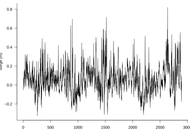
The Newlyn dataset consists of a series of 2894 measurements of sea-surge heights in meters that were taken over the period 1971 - 1976 at a location just off the coast at Newlyn, Cornwall, UK. The data represent the maximum hourly surge heights over periods of 15 hours (see Coles (1991)). Fawcett and Walshaw (2012) used this dataset to estimate the extremal index of the underlying process using several estimators and to make inferences about the extremes of the process. We proceed by first showing the Newlyn data in figure 5 below.
observation number Surge (m) 0 500 1000 1500 2000 2500 3000 −0.2 0.0 0.2 0.4 0.6 0.8
Figure 5: Time series plot of Newlyn sea-surge heights.
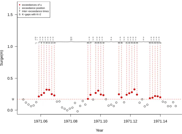
In figure 6 we illustrate the procedure of analysing the data using the K-gaps ex-ponential mixture model. For clarity and illustration purposes a small section of 60 observations (around the beginning of 1971) is shown and an 80% sample quantile was selected as threshold.
1.9 Thesis outline 41 ● ● ● ● ● ● ●● ● ● ● ●● ● ● ● ● ●● ● ● ● ● ● ● ● ● ● ●● ● ● ● ● ● ● ● ● ● ● ●● ● ● ● ● ● ●● ● ●● ● ● ● ● ● ● ● ● 1971.06 1971.08 1971.10 1971.12 1971.14 0.0 0.5 1.0 1.5 Year Surge(m) ●● ● ● ● ●● ● ● ● ● ● ● ● ● ●● ● ● ● ● ●● ● ● j = T = S = u ● j T S exceedances of u exceedance position Inter−exceedance times K−gaps with K=2 7 1 0 8 1 0 9 1 0 10 1 0 11 1 0 12 1 0 13 13 11 26 1 0 27 2 0 29 1 0 30 1 0 31 1 0 32 6 4 38 1 0 39 2 0 41 1 0 42 1 0 43 1 0 44 1 0 45 5 3 50 1 0 51 1 0 52 1 0 53 1 0 54
Figure 6: Time series plot of a segment of the Newlyn data illustrating threshold exceedances (red dots), exceedance locations (j), inter-exceedance times (T) and
K-gaps (S) forK = 2.
1.9
Thesis outline
The aim of this chapter was to introduce univariate extreme value theory and the statistical methods employed to make inferences using extreme value models. Fol-lowing the question we raised at the end of 1.5.2, chapter 2 considers the use of refer-ence priors in univariate extreme value modelling and present results concerning the propriety of posterior distributions. Furthermore, we consider different methods of performing Bayesian computation, i.e. sampling from the posterior distribution of model parameters and use a simulation study to compare different priors based on predictive inferences for future extreme values. Chapter 3 concerns threshold selec-tion for datasets of independent and identically distributed observaselec-tions. Bayesian cross-validation is used to compare single thresholds based on predictive ability at extreme levels and we proceed by using Bayesian model averaging to combine infer-ences from different thresholds. In chapter 4 we extend the approach developed in chapter 3 to the situation where independence is an unrealistic assumption and, in particular, extreme values tend to occur in clusters. Chapter 5 concerns threshold specification in extreme value regression modelling. In the context of a particular
model, a theoretical result concerning the optimality of quantile regression is de-rived. Chapter 6 summarises the main conclusion of this thesis and discusses some possible directions for future research.