For Peer Review
Journal: IEEE Transactions on Neural Networks and Learning Systems
Manuscript ID TNNLS-2018-P-8972 Manuscript Type: Paper
Date Submitted by the Author: 21-Jan-2018
Complete List of Authors: Ma, Zhanyu; Beijing University of Posts and Telecommunications, Pattern Recognition and Machine Intelligenc Lab.
Lai, Yuping; North China University of Technology, Department of Information Security
Kleijn, W. Bastiaan; Victoria University of Wellington, School of Engineering and Computer Science
Song, YiZhe; Queen Mary University of London, Wang, Liang; CASIA, NLPR
Guo, Jun; Beijing University of Posts and Telecommunications, Pattern Recognition and Machine Intelligenc Lab.
Keywords: Dirichlet process mixture, inverted Dirichlet distribution, Bayesian estimation, variational learning, computer vision
For Peer Review
1
Variational Bayesian Learning for Dirichlet Process
Mixture of Inverted Dirichlet Distributions
Zhanyu Ma, Senior Member, IEEE, Yuping Lai, Member, IEEE, W. Bastiaan Kleijn, Fellow, IEEE,
Yi-Zhe Song, Member, IEEE, Liang Wang, Senior Member, IEEE, and Jun Guo
Abstract—In this work, we develop a novel variational Bayesian learning method for the Dirichlet process (DP) mixture of the inverted Dirichlet distributions, which has been shown to be very flexible for modeling vectors with positive elements. The recently proposed extended variational inference (EVI) framework is adopted to derive an analytically tractable solution. The convergency of the proposed algorithm is theoretically guaranteed by introducing single lower bound approximation to the original objective function in the EVI framework. In principle, the proposed model can be viewed as an infinite inverted Dirichelt mixture model (InIDMM) that allows the automatic determination of the number of mixture components from data. Therefore, the problem of pre-determining the optimal number of mixing components has been overcome. Moreover, the problems of over-fitting and under-fitting are avoided by the Bayesian estimation approach. Comparing with several recently proposed DP-related methods and conventional applied methods, the good performance and effectiveness of the proposed method have been demonstrated with both synthesized data and real data evaluations.
Index Terms—Dirichlet process mixture, inverted Dirichlet distribution, Bayesian estimation, variational learning, computer vision
I. INTRODUCTION
Finite mixture modeling [1], [2] is a flexible and powerful probabilistic modeling tool for data that are assumed to be generated from heterogeneous populations. It has been widely applied to many areas, such as pattern recognition, machine learning, data mining, computer vision [3]–[7]. Among all finite mixture models, the finite Gaussian mixture model (GM-M) has been the most popular method for modeling continuous data. Much of its popularity is due to the fact that any continuous distribution can be arbitrarily well approximated by a GMM with unlimited number of mixture components. Moreover, the parameters in a GMM can be estimated ef-ficiently via maximum likelihood (ML) estimation with the expectation maximum (EM) algorithm [8]. By assigning prior distributions to the parameters in a GMM, Bayesian estimation of GMM can be carried out with conjugate prior-posterior
Z. Ma and J. Guo are with the Pattern Recognition and Intelligent System Lab., Beijing University of Posts and Telecommunications, Beijing, China.
Y. Lai is with the Department of Information Security, North China University of Technology, Beijing, China.
W. B. Kleijn is with the Communications and Signal Processing Group, Victoria University of Wellington, New Zealand.
Y.-Z. Song is with the SketchX Lab, School of Electronic Engineering and Computer Science, Queen Mary University of London, London, UK.
L. Wang is with the National Lab of Pattern Recognition, Institute of Automation, Chinese Academy of Sciences, Beijing, China.
The corresponding authors are Z. Ma (mazhanyu@bupt.edu.cn) and Y. Lai (laiyp@ncut.edu.cn).
pair matching [9], [10]. Both the ML and the Bayesian esti-mation algorithms can be represented in analytically tractable form [9].
Recent studies have shown that non-Gaussian statistical models, e.g., the beta mixture model (BMM) [6], the Dirichlet mixture model (DMM) [7], the Gamma mixture model (GaM-M) [11], the von Mises-Fisher mixture model (vM(GaM-M) [12], can model the non-Gaussian distributed data more efficiently, compared to the conventional GMM. For example, BMM has been widely applied in modeling grey image pixel values [6] and DNA methylation data [13]. In order to efficiently model proportional data [7], [14], DMM can be utilized to describe
the underlying distribution. In generalized-K (KG) fading
channels, GaMM has been used to analyze the capacity and error probability [11]. The vMM has been widely used in modeling directional data, such as yeast gene expression [12] and topic detection [15]. The finite inverted Dirichlet mixture model (IDMM), among others, has been demonstrated to be an efficient tool for modeling data vector with positive ele-ments [16], [17]. Moreover, the inverted Dirichlet distribution also has connections with nonnegative matrix factorization
(NMF). In sparse NMF [18], thel1-norm constraint is usually
applied to favor the sparseness. As the definition of the inverted Dirichlet distribution is similar to the nonnegative properties of the columns in the original matrix and the basis matrix, selecting proper prior distribution to describe the underlying distribution of the aforementioned columns can favor the sparse NMF.
An essential problem in finite mixture modeling is how to automatically decide the appropriate number of mixture components based on the data. The component number has a strong effect on the modeling accuracy [19]. If the number of mixture components is not properly chosen, the mixture model may over-fit or under-fit the observed data. To deal with this problem, many methods have been proposed. These can be categorized into two groups: deterministic approaches [20], [21] and Bayesian methods [22], [23]. Deterministic approach-es are generally implemented by ML approach-estimation under an EM-based and require the integration of entropy measures or some information theoretic criteria, such as the minimum mes-sage length (MML) [21], the Bayesian information criterion (BIC) [24], and the Akaike information criterion (AIC) [25], to determine the number of components in the mixture model. It is worth noting that, in general, the EM algorithm converges to a local maximum or a saddle point and its solution is highly dependent on its initialization. On the other hand, the Bayesian methods, which are not sensitive to initialization
4 5 6 7 8 9 10 11 12 13 14 15 16 17 18 19 20 21 22 23 24 25 26 27 28 29 30 31 32 33 34 35 36 37 38 39 40 41 42 43 44 45 46 47 48 49 50 51 52 53 54 55 56 57 58 59 60
For Peer Review
by introducing proper prior distributions to the parameters in the model, have been widely used to find a suitable number of components in a finite mixture model. In this case, the parameters of a finite mixture model (including the parameters in a component and the weighting coefficients) are treated as random variables under the Bayesian framework. The poste-rior distributions of the parameters, rather than simple point estimates, are computed [2]. The model truncation in Bayesian estimation of finite mixture model is carried out by setting the corresponding weights of the unimportant mixture components to zero (or a small value close to zero) [2]. However, the number of mixture components should be properly initialized, as it can only decrease during the training process.
The increasing interest in mixture modeling has led to the
development of the model selection method1. Recent work has
shown that the non-parametric Bayesian approach [26]–[30] can provide an elegant solution for automatically determining the complexity of model. The basic idea behind this approach is that it provides methods to adaptively select the optimal number of mixing components, while also allows the number of mixture components to remain unbounded. In other words, this approach allows the number of components to increase as new data arrives, which is the key difference from finite mixture modeling. The most widely used Bayesian nonpara-metric [31] model selection method is based on the Dirichlet process (DP) mixture model [32], [33]. The DP mixture model extends distributions over measures, which has the appealing property that it does not need to set a prior on the number of components. In essence, the DP mixture model can also be viewed as an infinite mixture model with its complexity increasing as the size of dataset grows. Recently, the DP mix-ture model has been applied in many important applications. For instance, the DP mixture model has been adopted to a mixture of different types of non-Gaussian distributions, such as the DP mixture of beta-Liouville distributions [34], the DP mixture of student’s-t distributions [35], the DP mixture of generalized Dirichlet distributions [36], the DP mixture of student’s-t factors [37], and the DP mixture of hidden Markov random field models [38].
Generally speaking, most parameter estimation algorithms for both the deterministic and the Bayesian methods are time consuming, because they have to numerically evaluate a given model selection criterion [21]. This is especially true for the fully Bayesian Markov chain Monte Carlo (MCMC) [27], [39], which is one of the widely applied Bayesian approaches with numerical simulations. The MCMC approach has its own limitations, when high-dimensional data are involved in the training stage [40]. This is due to the fact that its sampling-based characteristics yield a heavy computational burden and it is difficult to monitor the convergence in the high-dimensional space. To overcome the aforementioned problems, variational inference (VI), which can provide an analytically tractable solution and good generalization performance, has been pro-posed as an efficient alternative to the MCMC approach [41]. With an analytically tractable solution, the numerical sampling
1Here, model selection means selecting the best of a set of models of
different orders
during each iteration in the optimization stage can be avoided. Hence, the VI-based solutions can lead to more efficient estimation. They have been successfully applied in a variety of applications including the estimation of mixture models [5]– [7], [34], [42].
Motivated by the ability of the Bayesian non-parametric approaches to solve the model selection problem and the good performance recently obtained by the VI framework, we focus on the variational learning of the DP mixture of inverted Dirichlet distributions (a.k.a. the infinite inverted Dirichlet mixture model (InIDMM)). Since InIDMM is a typical non-Gaussian statistical model, it is not feasible to apply the standard VI framework to obtain an analytically tractable solution for the Bayesian estimation. As a variate of VI, stochastic variational infernece (SVI) [43], [44] has been proposed as an alternative solution to approximate the posterior distributions. The algorithm under SVI framework is scalable and suitable for massive data. However, when dealing with non-Gaussian distributions, the expectations in the update
iterations (Fig. 4, [43]) cannot be calculated explicitly and
some sampling methods are also required to approximate the expectations. In order to derive an analytically tractable solution for the variational learning of InIDMM, the recently proposed extended variational inference (EVI) [6], [7], which is particularly suitable for non-Gaussian statistical models, has been adopted to provide an appropriate single lower bound
(SLB) approximation to the original object function. With
the auxiliary function, an analytically tractable solution for Bayesian estimation of InIDMM is derived. The key contribu-tions of our work are three-fold: 1) The finite inverted Dirichlet mixture model (IDMM) has been extended to the infinite inverted Dirichlet mixture model (InIDMM) under the stick-breaking process framework [32], [45]. Thus, the difficulty in automatically determining the number of mixture components can be overcome. 2) An analytically solution is derived with the EVI framework for InIDMM. Moreover, comparing with the recently proposed algorithm for InIDMM [46], which is based on multiple lower bound (MLB) approximation, our algorithm can not only theoretically guarantee convergence but also provide better approximations. 3) The proposed method has been applied in several important applications in computer vision, such as image categorization and object detection. The good performance has been illustrated with both synthesized and real data evaluations.
The remaining part of this paper is organized as follow: Sec-tion II provides a brief overview of the finite inverted Dirichlet mixture and the DP mixture. The infinite inverted Dirichlet mixture model is also proposed. In Section III, a Bayesian learning algorithm with EVI is derived. The proposed algorith-m has an analytically tractable foralgorith-m. The experialgorith-mental results with both synthesized and real data evaluations are reported in Section IV. Finally, we draw conclusions and future research directions in Section V.
II. THE STATISTICAL MODEL
In this section, we first present a brief overview of the finite inverted Dirichlet mixture model (IDMM). Then, the DP
mix-6 7 8 9 10 11 12 13 14 15 16 17 18 19 20 21 22 23 24 25 26 27 28 29 30 31 32 33 34 35 36 37 38 39 40 41 42 43 44 45 46 47 48 49 50 51 52 53 54 55 56 57 58 59 60
For Peer Review
3
ture model with stick-breaking representation is introduced. Finally, we extend the IDMM to InIDMM.
A. Finite inverted Dirichlet mixture model
Given a D-dimensional vector~x={x1,· · ·, xD}generated
from an IDMM with M components, the probability density
function (PDF) of~xis denoted as [16] IDMM(~x|~π,Λ) = M X m=1 πmiDir(~x|~αm), (1)
where Λ = {~αm}Mm=1 and ~π = {πm}Mm=1 is the mixing
coefficient vector subject to the constraints 0≤πm ≤1 and
PM
m=1πm= 1. Moreover, iDir(~x|α)~ is an inverted Dirichlet
distribution with its (D+ 1)-dimensional positive parameter
vector ~α={α1,· · ·, αD+1} defined as iDir(~x|~α) = Γ( PD+1 d=1 αd) QD+1 d=1 Γ(αd) D Y d=1 xαd−1 d 1 + D X d=1 xd !−PDd=1+1αd , (2)
where xd > 0 for d = 1,· · · , D and Γ(·) is the Gamma
function defined asΓ(a) =R0∞ta−1e−tdt.
B. Dirichlet Process with Stick-Breaking
The Dirichlet process (DP) [32], [33] is a stochastic process used for Bayesian nonparametric data analysis, particularly in a DP mixture model (infinite mixture model). It is a distribution over distributions rather than parameters, i.e., each draw from a DP is a probability distribution itself, rather than a parameter vector [47]. We adopt the DP to extend the IDMM to the infinite case, such that the difficulty of the automatic determination of the model complexity (i.e., the number of mixture components) can be overcome. To this end, the DP is constructed by the following stick-breaking formulation [31], [48], [49], which is an intuitive and simple constructive definition of the DP.
Assume thatH is a random distribution andϕis a positive
real scalar. We consider two countably infinite collections
of independently generated stochastic variables Ωm ∼ H
and λm ∼ Beta(λm; 1, ϕ)2 for m = {1,· · ·,∞}, where
Beta(x;a, b)is the beta distribution defined as Beta(x;a, b) =
Γ(a+b) Γ(a)Γ(b)xa−
1(1−x)b−1. A distribution G is said to be DP
distributed with a concentration parameter ϕ and a base
measure or base distribution H (denoted asG∼DP(ϕ, H)),
if the following conditions are satisfied:
G= ∞ X m=1 πmδΩm, πm=λm mY−1 l=1 (1−λl), (3)
where{πm}is a set of stick-breaking weights with constraints
P∞
m=1πm= 1, δΩm is a delta function whose value is 1 at
location Ωm and 0 otherwise. The generation of the mixing
coefficients {πm} can be considered as process of breaking
a unit length stick into an infinite number of pieces. The
2To avoid confusion, we usef(x;a)to denote the PDF ofxparameterized
by parametera.f(x|a)is used to denote the conditional PDF ofxgivena, where both xandaare random variables. Bothf(x;a)andf(x|a)have exactly the same mathematical expressions.
~zn ∞ ∞ ∞ λm ϕm ~ αm N ~xn
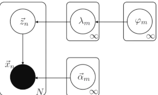
Fig. 1: Graphical representation of the variables relationships in the Bayesian inference of a InIDMM. All of the circles in the graphical figure represent variables. Arrows show the relationships between variables. The variables in the box are the i.i.d. observations.
length of each piece, λm, which is proportional to the rest
of the “stick” before the current breaking, is considered as an
independent random variable generated from Beta(λm; 1, ϕ).
Because of its simplicity and natural generalization ability, the stick-breaking construction has been a widely applied scheme for the inference of DPs [34], [45], [50].
C. Infinite Inverted Dirichlet Mixture Model
Now we consider the problem of modeling~xby an Infinite
Inverted Dirichlet Mixture Model (InIDMM), which is actually an extended IDMM with an infinite number of components. Therefore, (1) can be reformulated as
InIDMM(~x|~π,Λ) =
∞
X m=1
πmiDir(~x|~αm), (4)
where ~π = {πm}∞m=1 and Λ = {α~m}∞m=1. Then, the
likelihood function of the InIDMM given the observed dataset
X ={~xn}Nn=1 is given by InIDMM(X |~π,Λ) = N Y n=1 (X∞ m=1 πmiDir(~xn|~αm) ) . (5)
In order to clearly illustrate the generation process of each
observation ~xn in the mixture model, we introduce a latent
indication vector variable ~zn = {zn1, zn2,· · · }. ~z has only
one element equal to1 and the other elements in~z are0. For
example, znm = 1 indicates the sample ~xn comes from the
mixture componentm. Therefore, the conditional distribution
of X given the parameters Λ and the latent variables Z =
{znm} is InIDMM(X |Z,Λ) = N Y n=1 ∞ Y m=1 iDir(~xn|~αm)znm. (6)
Moreover, to exploit the advantages of the Bayesian frame-work, conjugate prior distributions are introduced for all the unknown parameters according to their distribution properties. In this work, we place the conjugate priors over the unknown
stochastic variables Z, Λ, and ~λ = (λ1, λ2,· · ·) such that a
full Bayesian estimation model can be obtained.
In the aforementioned full Bayesian model, the prior
distri-bution ofZ given~πis given by
p(Z|~π) = N Y n=1 ∞ Y m=1 πznm m . (7) 4 5 6 7 8 9 10 11 12 13 14 15 16 17 18 19 20 21 22 23 24 25 26 27 28 29 30 31 32 33 34 35 36 37 38 39 40 41 42 43 44 45 46 47 48 49 50 51 52 53 54 55 56 57 58 59 60
For Peer Review
As ~π is a function of ~λ according to the stick-breaking
construction of the DP as shown in (3), we rewrite (7) as
p(Z|~λ) = N Y n=1 ∞ Y m=1 " λm mY−1 l=1 (1−λl) #znm . (8)
As previously mentioned in Section II-B, the prior
distribu-tion of~λ is p(~λ|ϕ~) = ∞ Y m=1 Beta(λm; 1, ϕm) = ∞ Y m=1 ϕm(1−λm)ϕm−1, (9)
where ϕ~ = (ϕ1, ϕ2,· · ·). Based on (3), we can obtain the
expected value ofπm. In order to do this, the expected value
ofλmwill first be calculated as
hλmi= 1/(1 +ϕm). (10)
Then, the expected value of πm is denoted as
hπmi=hλmi mY−1
l=1
(1− hλli). (11)
It is worth to note that, when the value ofϕmis small,hλmi
will become large. Therefore, the expected of the mixing
co-efficientsπm are controlled by the parametersϕm, i.e., small
value ofϕmwill yield smallπmsuch that the distribution of
πmwill be sparse.
Asϕmis positive, we assumeϕ~follows a product of gamma
prior distributions as p(ϕ~;~s, ~t) = ∞ Y m=1 Gam(ϕm;sm, tm) = ∞ Y m=1 tsm m Γ(sm) ϕsm−1 m e−tmϕm, (12)
where Gam(·) is the gamma distribution. ~s = (s1, s2,· · ·)
and~t= (t1, t2,· · ·)are the hyperparamters and subject to the
constraintssm>0andtm>0.
Next, we introduce an approximating conjugate prior
dis-tribution to parameter Λ in InIDMM. The inverted Dirichlet
distribution belongs to the exponential family and its formal conjugate prior can be derived with the Bayesian rule [2] as
p(~α|~µ0, v0) =C(~µ0, v0) " Γ(PDd=1+1αd) QD+1 d=1 αd #ν0 e−~µ0(~αT−I~D+1), (13)
where ~µ0= [µ10,· · ·µD+10] andν0 are the hyperparameters
in the prior distribution, C(~µ0, v0) is a normalization
coeffi-cient such that Rp(~α|~µ0, v0)d~α = 1.I~d is a D-dimensional
vector with all elements equal to one. Then, we can write the
posterior distribution ofα~ as (with N i.i.d. observationsX)
f(~α|X) =R iDir(X |α~)f(α~|~µ0, ν0) iDir(X |α~)f(α~|~µ0, ν0)d~α =C(~µN, νN) " Γ(PDd=1+1αd) QD+1 d=1 Γ(αd) #νN e−~µN(~αT−~ID+1) (14)
where the hyperparametersνN and~µN in the posterior
distri-bution are
νN=ν0+N, ~µN=~µ0−[lnX+−~ID+1ln(1 +~IDT+1X+)]~IN.
(15)
In (15), X+ is a (D+ 1)×N matrix by connecting I~T
D+1
to the bottom of X. However, it is not applicable in our VI
framework due to the analytically intractable normalization
factor in (44). Because Λ is positive, we adopt gamma prior
Model estimation strategies for IDMM
Model estimation strategies for InIDMM
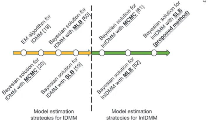
Fig. 2:Development progress of the model estimation strategies for
finite IDMM and infinite IDMM.
distributions to approximate conjugate prior forΛas well. By
assuming the parameters of inverted Dirichlet distribution are mutually independent, we have
p(Λ) =Gam(Λ;U, V) = ∞ Y m=1 DY+1 d=1 vumd md Γ(umd) αumd−1 md e −vmdαmd , (16)
where all the hyperparametersU = {umd} andV ={vmd}
are positive.
With the Bayesian rules and by combining (6) and (8)-(16) together, we can represent the joint density of the observation
X with all thei.i.d.latent variablesΘ = (Z,Λ, ~λ, ~ϕ)as
p(X,Θ) =p(X |Z,Λ)p(Z|~λ)p(~λ|ϕ~)p(ϕ~)p(Λ) = N Y n=1 ∞ Y m=1 λm mY−1 j=1 (1−λj) ΓPDd=1+1αmd QD+1 d=1 Γ(αmd) × D Y d=1 xαmd−1 nd 1 + D X d=1 xnd !−PD+1 d=1 αmd znm × ∞ Y m=1 ϕm(1−λm)ϕm−1 tsm m Γ(sm) ϕsm−1 m e −tmϕm × ∞ Y m=1 DY+1 d=1 vumd md Γ(umd) αumd−1 md e −vmdαmd . (17) The structure of the InIDMM can be represented in terms of a graphical model in Fig. 1. The development progress for the related models are shown in Fig. 2.
III. VARIATIONALLEARNING FORINIDMM
In this section, we develop a variational Bayesian inference framework for learning the InIDMM. With the assistance of recently proposed EVI [6], [7], an analytically tractable algorithm, which prevents numerical sampling during each iteration and facilitates a training procedure, is obtained. The proposed solution is also able to overcome the problem of overfitting and automatically decide the number of mixture components.
A. Extended Variational Inference
The purpose of Bayesian analysis is to estimate the values of the hyperparameters as well as the posterior probability distribution of the latent variables. Within the conventional
6 7 8 9 10 11 12 13 14 15 16 17 18 19 20 21 22 23 24 25 26 27 28 29 30 31 32 33 34 35 36 37 38 39 40 41 42 43 44 45 46 47 48 49 50 51 52 53 54 55 56 57 58 59 60
For Peer Review
5
variational inference framework, the objective function that needs to be maximized is
L(q) =Eq(Θ)[lnp(X,Θ)]−Eq(Θ)[lnq(Θ)]. (18) For most of the non-Gaussian mixture models (e.g., the beta mixture model [7], the Dirichlet mixture model [6], the beta-Liouville mixture model [34], the inverted Dirichlet mixture
model [17]), the term Eq(Θ)[lnp(X,Θ)] is analytically
in-tractable such that the lower boundL(q)cannot be maximized
directly by a closed-form solution. Therefore, the EVI method [6], [7], [41] was proposed to overcome the aforementioned
problem. With an auxiliary function p(˜X,Θ) that satisfies
Eq(Θ)[lnp(X,Θ)]≥Eq(Θ)[ln ˜p(X,Θ)] (19) and substituting (19) into (18), we can still reach the maximum
value of L(q) at some given points by maximizing a lower
bound of L˜(q)
L(q)≥L˜(q) =Eq(Θ)[ln ˜p(X,Θ)]−Eq(Θ)[lnq(Θ)]. (20)
If p(˜X,Θ) is properly selected, an analytically tractable
so-lution can be obtained. In order to properly formulate the
variational posterior q(Θ), we truncate the stick-breaking
representation for the InIDMM at a value M as
λM = 1, πm= 0 whenm > M, and
M X m=1
πm= 1. (21)
Note that the model is still a full DP mixture. The truncation
levelM is not a part of our prior infinite mixture model, it is
only a variational parameter for pursuing an approximation to the posterior, which can be freely initialized and automatically optimized without yielding overfitting during the learning process. Additionally, we make use of the following factorized
variational distribution to approximatep(Θ|X)as
q(Θ) = M Y m=1 q(λm)q(ϕm) N Y n=1 q(znm) DY+1 d=1 q(αmd), (22)
where the variables in the posterior distribution are assumed to be mutually independent (as illustrated by the graphical model in Fig. 1). This is the only assumption we introduced to the posterior distribution. No other restrictions are imposed over the mathematical forms of the individual factor distribution-s [2].
Applying the full factorization formulation and the truncated stick-breaking representation for the proposed model, we can solve the variational learning by maximizing the lower bound
˜
L(q)shown in (20). The optimal solution in this case is given
by
lnqs(Θs) =hln ˜p(X,Θ)ij6=s+Con., (23)
where h·ij6=s refers to the expectation with respect to all the
distributionsqj(Θj)except for variables. In addition, any term
that does not includeΘsare absorbed into the additive constant
“Con.” [2], [41]. In the variational inference, all factorsqs(Θs)
need to be suitably initiated, then each factor is updated in turn with a revised value obtained by (23) using the current values of all the other factors. Convergence is theoretically guaranteed since the lower bound is a convex with respect to each factor
qs(Θs)[2], [6].
B. EVI for the Optimal Posterior Distributions
According to the principles of EVI, the expectation of the logarithm of the joint distribution, given the joint posterior distributions of the parameters, can be expressed as
hlnp(X,Θ)i = N X n=1 M X m=1 hznmi " Rm+ D X d=1 (hαmdi −1) lnxnd − DX+1 d=1 hαmdi(1 + D X d=1 xnd) +hlnλmi+ mX−1 j=1 hln(1−λj)i # + M X m=1 [hlnϕmi+ (hϕmi −1)hln(1−λm)i] + M X m=1 DX+1 d=1 (umd−1)hlnαmdi −vmdhαmdi + M X m=1 [(sm−1)hlnϕmi −tmhϕmi] +Con., (24) whereRm= D lnΓ( PD+1 d=1αmd) QD+1 d=1 Γ(αmd) E .
With the mathematical expression in (24), an analytically tractable solution is not feasible, which is due to the fact
that Rm cannot be explicitly calculated (although it can be
simulated by some numerical sampling methods). In order to apply (23) to explicitly calculate the optimal posterior distributions and with the principles of the EVI framework,
it is required to introduce an auxiliary functionR˜m such that
Rm≥R˜m. According to [6, Eq. 25], we can selectR˜m as
˜ Rm= ln Γ(PDd=1+1hαmdi) QD+1 d=1 Γ(hαmdi) + DX+1 d=1 " Ψ( DX+1 k=1 hαmdi)−Ψ(hαmdi) # ×[hlnαmdi −lnhαmdi]hαmdi, (25)
where Ψ(·) is the digamma function defined as Ψ(a) =
∂ln Γ(a)/∂a.
Substituting (25) into (24), a lower bound to hlnp(X,Θ)i
can be obtained as hln ˜p(X,Θ)i = N X n=1 M X m=1 hznmi " ˜ Rm+ D X d=1 (hαmdi −1) lnxnd − DX+1 d=1 hαmdi(1 + D X d=1 xnd) +hlnλmi+ mX−1 j=1 hln(1−λj)i # + M X m=1 [hlnϕmi+ (hϕmi −1)hln(1−λm)i] + M X m=1 DX+1 d=1 (umd−1)hlnαmdi −vmdhαmdi + M X m=1 [(sm−1)hlnϕmi −tmhϕmi] +Con.. (26) With (23), we can get analytically tractable solutions for
optimally estimating the posterior distributions of Z, ~λ, ϕ~,
andΛ. We now consider each of these in more detail: 1) The
posterior distribution of q(Z) 4 5 6 7 8 9 10 11 12 13 14 15 16 17 18 19 20 21 22 23 24 25 26 27 28 29 30 31 32 33 34 35 36 37 38 39 40 41 42 43 44 45 46 47 48 49 50 51 52 53 54 55 56 57 58 59 60
For Peer Review
As any term that is independent of znm can be absorbed
into the additive constant, we have
lnq∗(znm) =Con.+znm " e Rm+hlnλmi+ mX−1 j=1 hln(1−λj)i + D X d=1 (hαmdi −1) lnxnd+ DX+1 d=1 hαmdiln(1 + D X d=1 xnd) # , (27) which has same logarithmic form of the prior distribution (i.e.,
the categorial distribution). Therefore, we can writelnq∗(Z)
as lnq∗(Z) = N X n=1 M X m=1 znmlnρnm+Con. (28)
with the definition that
lnρnm=hlnλmi+ mX−1 j=1 hln(1−λj)i+ ˜Rm + D X d=1 (hαmdi −1) lnxnd− DX+1 d=1 hαmdi(1 + D X d=1 xnd). (29)
Recalling that znm∈(0,1)andPMm=1znm= 1, we define
rnm=
ρnm
PM m=1ρnm
. (30)
Taking the exponential of both sides of (28), we have
q∗(Z) = N Y n=1 M Y m=1 rznm nm , (31)
which is the optimal posterior distribution of Z.
The posterior mean hznmi can be calculated as hznmi =
rnm. Actually, the quantities{rnm}are playing a similar role
as the responsibilities in the conventional EM [51] algorithm. In the following parts, we show only the optimal solutions
to ~λ, ϕ~, and Λ, respectively. The derivation details can be
found in the appendix.
2) The posterior distribution of q(~λ)
The optimal solution to the posterior distribution of ~λ is
characterized as q(~λ) = M Y m=1 Beta(λm;gm∗, h ∗ m), (32)
where the hyperparameterss∗
m andqm∗ are g∗m= 1 + N X n=1 hznmi, h∗m=hϕmi+ N X n=1 M X j=m+1 hznji. (33)
3) The posterior distribution of q(~ϕ)
The optimal solution to the posterior distribution ofϕ~ is
q∗(ϕ~) = M Y m=1 Gam(ϕm;s∗m, t ∗ m), (34)
where the optimal solutions to the hyperparamterss∗
mandt∗m are s∗m= 1 +s 0 m, t ∗ m=t 0 m− hln(1−λm)i, (35) wheres0
mandt0mdenote the hyperparameters initialized in the
prior distribution, respectively.
4) The posterior distribution of q(Λ)
The optimal approximation to the posterior distribution of
Λis q∗(Λ) = M Y m=1 DY+1 d=1 Gam(αmd;u∗md, v ∗ md), (36)
where the optimal solutions to the hyperparametersu∗
md and v∗ md are given by u∗ md=u0md+ N X n=1 hznmi " Ψ( KX+1 k=1 hαmki)−Ψ(hαmdi) # hαmdi (37) and vmd∗ =v0md− N X n=1 hznmi " lnxnd−ln(1 + D X d=1 xnd) # . (38)
In the above equations,u0
mdandvmd0 are the hyperparameters
in the prior distribution and we setxn,D+1 = 1. The following
expectations are needed to calculate the aforementioned update equations: hln(1−λm)i=Ψ(h∗m)−Ψ(g ∗ m+h ∗ m), hlnλmi=Ψ(g∗m)−Ψ(g ∗ m+t ∗ m), hlnαmdi=Ψ(u∗md)−lnv ∗ md, hϕmi= s∗ m t∗ m ,hαmdi= u∗ md v∗ md . (39)
C. Full Variational Learning Algorithm
As can be observed from the above updating process, the optimal solutions for the posterior distributions are dependent on the moments evaluated with respect to the posterior dis-tributions of the other variables. Thus, the variational update equations are mutually coupled. In order to obtain optimal posterior distributions for all the variables, iterative updates are required until convergence. With the obtained posterior distributions, it is straightforward to calculate the lower bound
˜ L(q) ˜ L(q) = Z q(Θ) lnp˜(Θ,X) q(Θ) dΘ =hln ˜p(X,Θ)i − hlnq(Θ)i =hln ˜p(X,Θ)i − hlnq(Z)i − hlnq(~λ)i − hlnq(ϕ~)i − hlnq(Λ)i, (40)
which is helpful in monitoring the convergence. In (40), each
term with expectation (i.e.,h·i) is evaluated with respect to all
the variables in its argument as
hlnq(Z)i=rnmlnrnm, (41) hlnq(~λ)i= M X m=1 [ln Γ(gm∗ +h ∗ m)−ln Γ(g ∗ m)−ln Γ(h ∗ m) +(g∗m−1)hlnλmi+ (h∗m−1)hln(1−λm)i], (42) hlnq(ϕ~)i= M X m=1 [s∗ mlnt∗m−ln Γ(s∗m) +(s∗ m−1)hlnϕmi −t∗mϕ¯m], (43) and hlnq(α~)i= M X m=1 DX+1 d=1 [u∗mdlnv ∗ md−ln Γ(u ∗ m) +(u∗ m−1)hlnαmdi −v∗mdα¯md]. (44) 6 7 8 9 10 11 12 13 14 15 16 17 18 19 20 21 22 23 24 25 26 27 28 29 30 31 32 33 34 35 36 37 38 39 40 41 42 43 44 45 46 47 48 49 50 51 52 53 54 55 56 57 58 59 60
For Peer Review
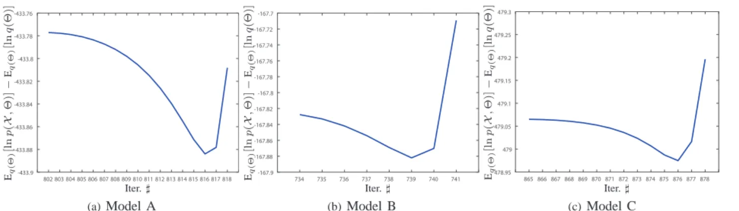
7 802 803 804 805 806 807 808 809 810 811 812 813 814 815 816 817 818 -433.9 -433.88 -433.86 -433.84 -433.82 -433.8 -433.78 -433.76 Iter.♯ Eq ( Θ ) [l n p ( X , Θ )] − Eq ( Θ ) [l n q (Θ )] (a)Model A 734 735 736 737 738 739 740 741 -167.9 -167.88 -167.86 -167.84 -167.82 -167.8 -167.78 -167.76 -167.74 -167.72 -167.7 Iter.♯ Eq ( Θ ) [l n p ( X , Θ )] − Eq ( Θ ) [l n q (Θ )] (b)Model B 865 866 867 868 869 870 871 872 873 874 875 876 877 878 478.95 479 479.05 479.1 479.15 479.2 479.25 479.3 Iter.♯ Eq ( Θ ) [l n p ( X , Θ )] − Eq ( Θ ) [l n q (Θ )] (c)Model CFig. 3: Observations of the objective function’s oscillations during iterations. This non-convergence indicates that the MLB
approximation-based method cannot theoretically guarantee convergence. The model settings are the same as Tab. I.
Algorithm 1 Algorithm for EVI-based Bayesian InIDMM
1: Set the initial truncation levelM and the initial values for
hyperparameterss0
m,t0m,u0md, andv0md
2: Initialize the values ofrnm by K-means algorithm.
3: repeat
4: Calculate the expectations in (39).
5: Update the posterior distributions for each variable by
(33), (35), (37) and (38).
6: until Stop criterion is reached.
7: For all m, calculatehλmi=s∗m/(s∗m+t∗m) and
substi-tute it back into (11) to get the estimated values of the
mixing coefficientsπbm.
8: Determine the optimum number of components M by
eliminating the components with mixing weights smaller
than10−5.3
9: Renormalize{bπm}to have a unit l1 norm.
10: Calculate αbmd=umd∗ /vmd∗ for allmandd.
Additionally,hln ˜p(X,Θ)iis given in (26) .
The algorithm of the proposed EVI-based Bayesian estima-tion of InIDMM is summarized in Algorithm 1.
IV. EXPERIMENTALRESULTS ANDDISCUSSIONS
In this section, both synthesized data and real data are utilized to demonstrate the performance of the proposed al-gorithm for InIDMM. In the initialization stage of all the
experiments, the truncation level M is set to 15 and the
hyperparameters of the gamma prior distributions are chosen as u0 =s0 = 1 andv0 = t0 = 0.005, which provide
non-informative prior distributions. Note that these specific choices were based on our experiments and were found convenient and effective in our case. We take the posterior means as point estimates to the parameters in an InIDMM.
A. Synthesized Data Evaluation
As shown in the previous studies for EVI-based Bayesian estimation [5], [6], the SLB approximation can guarantee the convergence while the MLB approximation cannot. We use the
3When a mixing coefficient is small enough, it converges to0faster.
There-fore, we can remove components with very small value (less than a threshold). This choice (empirically choosing a threshold) is purely for the convenience of easy implementation. Similar strategy is also widely used applied in many other sticking-break process-based DP mixture models, e.g., [34], [46].
synthesized data evaluation to compare the Bayesian InIDMM using the SLB approximation (proposed in this paper and
denoted as InIDMMSLB) with the Bayesian InIDMM using
the MLB approximation (proposed in [46] and denoted as
InIDMMMLB). Three models (see Tab. I for details) were
selected to generate the synthesized datasets.
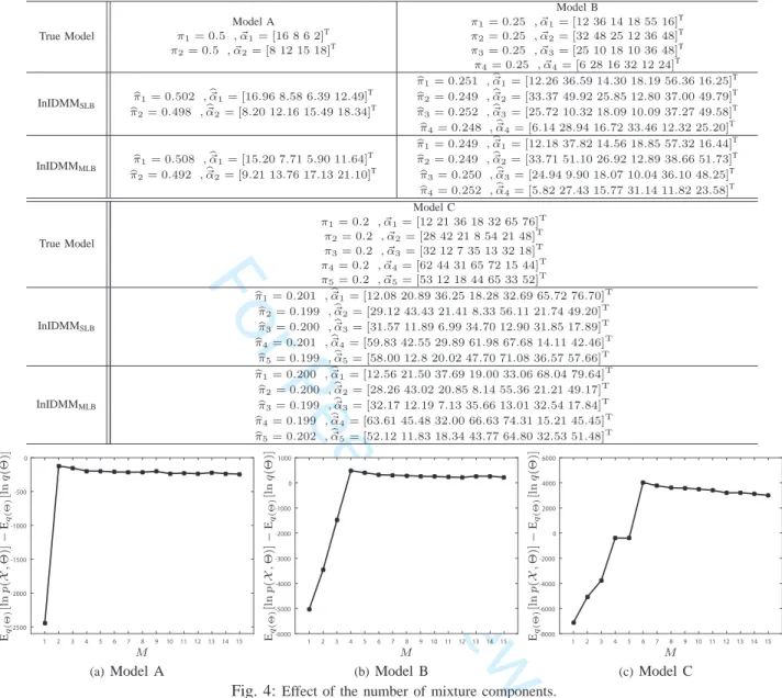
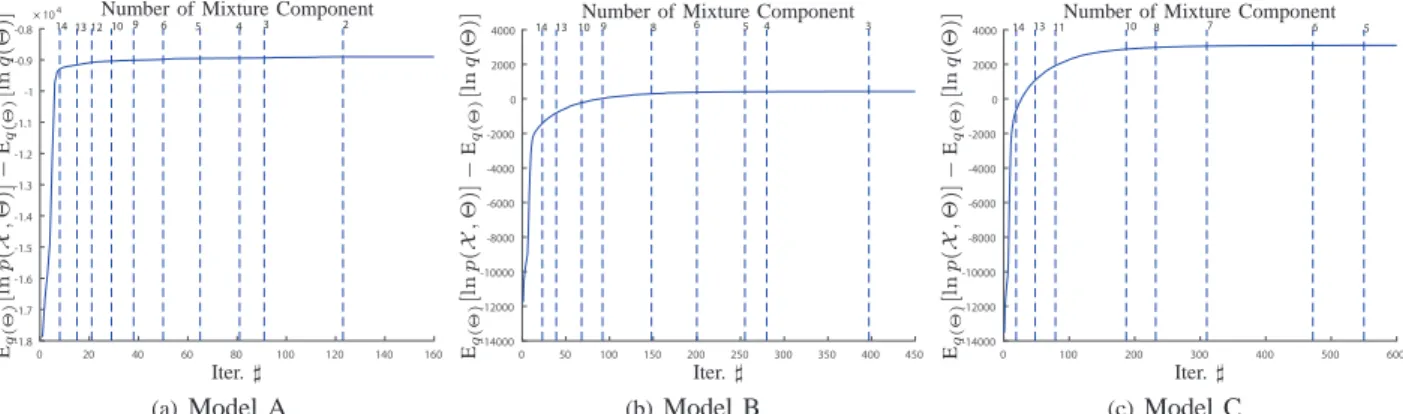
1) Model Selection: One advantage of DP process
mix-ture model is to decide the number of mixmix-ture components automatically, based on the training data. Following the in-structions in [52] and for a first check, we ran the proposed
EVI-based method for InIDMMSLB. The optimization
pro-cedure is carried out without component elimination (i.e., a
fixed number of components, M, is chosen and the mixing
coefficients are fixed during iteration. The initial value of the mixing coefficients were obtained from plain EM estimation.) Under this setting, the variational lower-bound can be treated as a model selection score and the effect of the number of the mixture components is demonstrated. With synthesized data generated from the aforementioned three models, we plotted the relation between the variaional lower-bounds and the number of mixture components in Fig. 4.
2) Observations of Oscillations: We ran the InIDMMMLB
algorithm and monitored the value of the variational objective function during each iteration. It can be observed that the variational objective function was not always increasing in
Bayesian estimation with the InIDMMMLB. Figure 3 illustrates
the decreasing values during iterations. On the other hand, the
variational objective function obtained with the InIDMMSLB
algorithm was always increasing until convergence, as the SLB approximation insures the convergency theoretically. The observations of oscillations demonstrate that the convergence with MLB approximation cannot be guaranteed. The original variational object function was numerically calculated by employing sampling method. In order to monitor the parameter
estimation process of InIDMMSLB, we show the value of the
variational objective function during iterations in Fig. 5. It can be observe that the variational objective function obtained by
InIDMMSLB increases during iterations and in most cases it
increases very fast.
3) Quantitative Comparisons: Next, we compare the
InIDMMSLB with the InIDMMMLB quantitatively. With
a known IDMM, 2000 samples were generated. The
InIDMMSLB and the InIDMMMLB were applied to estimate
the posterior distributions of the model, respectively. In Tab. I,
4 5 6 7 8 9 10 11 12 13 14 15 16 17 18 19 20 21 22 23 24 25 26 27 28 29 30 31 32 33 34 35 36 37 38 39 40 41 42 43 44 45 46 47 48 49 50 51 52 53 54 55 56 57 58 59 60
For Peer Review
TABLE I: Comparisons of true and estimated models.
True Model Model A π1= 0.5 , ~α1= [16 8 6 2]T π2= 0.5 , ~α2= [8 12 15 18]T Model B π1= 0.25 , ~α1= [12 36 14 18 55 16]T π2= 0.25 , ~α2= [32 48 25 12 36 48]T π3= 0.25 , ~α3= [25 10 18 10 36 48]T π4= 0.25 , ~α4= [6 28 16 32 12 24]T InIDMMSLB bπ1= 0.502 , b ~ α1= [16.96 8.58 6.39 12.49]T b π2= 0.498 ,~αb2= [8.20 12.16 15.49 18.34]T b π1= 0.251 ,αb~1= [12.26 36.59 14.30 18.19 56.36 16.25]T b π2= 0.249 ,αb~2= [33.37 49.92 25.85 12.80 37.00 49.79]T b π3= 0.252 ,αb~3= [25.72 10.32 18.09 10.09 37.27 49.58]T b π4= 0.248 ,αb~4= [6.14 28.94 16.72 33.46 12.32 25.20]T InIDMMMLB b π1= 0.508 ,αb~1= [15.20 7.71 5.90 11.64]T b π2= 0.492 ,~αb2= [9.21 13.76 17.13 21.10]T b π1= 0.249 ,αb~1= [12.18 37.82 14.56 18.85 57.32 16.44]T b π2= 0.249 ,αb~2= [33.71 51.10 26.92 12.89 38.66 51.73]T b π3= 0.250 ,αb~3= [24.94 9.90 18.07 10.04 36.10 48.25]T b π4= 0.252 ,αb~4= [5.82 27.43 15.77 31.14 11.82 23.58]T True Model Model C π1= 0.2 , ~α1= [12 21 36 18 32 65 76]T π2= 0.2 , ~α2= [28 42 21 8 54 21 48]T π3= 0.2 , ~α3= [32 12 7 35 13 32 18]T π4= 0.2 , ~α4= [62 44 31 65 72 15 44]T π5= 0.2 , ~α5= [53 12 18 44 65 33 52]T InIDMMSLB b π1= 0.201 ,b~α1= [12.08 20.89 36.25 18.28 32.69 65.72 76.70]T b π2= 0.199 ,b~α2= [29.12 43.43 21.41 8.33 56.11 21.74 49.20]T b π3= 0.200 ,b~α3= [31.57 11.89 6.99 34.70 12.90 31.85 17.89]T b π4= 0.201 ,b~α4= [59.83 42.55 29.89 61.98 67.68 14.11 42.46]T b π5= 0.199 ,b~α5= [58.00 12.8 20.02 47.70 71.08 36.57 57.66]T InIDMMMLB b π1= 0.200 ,b~α1= [12.56 21.50 37.69 19.00 33.06 68.04 79.64]T b π2= 0.200 ,b~α2= [28.26 43.02 20.85 8.14 55.36 21.21 49.17]T b π3= 0.199 ,b~α3= [32.17 12.19 7.13 35.66 13.01 32.54 17.84]T b π4= 0.199 ,b~α4= [63.61 45.48 32.00 66.63 74.31 15.21 45.45]T b π5= 0.202 ,b~α5= [52.12 11.83 18.34 43.77 64.80 32.53 51.48]T 1 2 3 4 5 6 7 8 9 10 11 12 13 14 15 -2500 -2000 -1500 -1000 -500 0 M Eq ( Θ ) [l n p ( X , Θ )] − Eq ( Θ ) [l n q (Θ )] (a)Model A 1 2 3 4 5 6 7 8 9 10 11 12 13 14 15 -6000 -5000 -4000 -3000 -2000 -1000 0 1000 M Eq ( Θ ) [l n p ( X , Θ )] − Eq ( Θ ) [l n q (Θ )] (b)Model B 1 2 3 4 5 6 7 8 9 10 11 12 13 14 15 -8000 -6000 -4000 -2000 0 2000 4000 6000 M Eq ( Θ ) [l n p ( X , Θ )] − Eq ( Θ ) [l n q (Θ )] (c)Model C
Fig. 4:Effect of the number of mixture components.
TABLE II: Comparisons of objective function values and runtime for InIDMM with SLB and MLB.
Model&Method InIDMM Model A Model B Model C
SLB InIDMMMLB InIDMMSLB InIDMMMLB InIDMMSLB InIDMMMLB
Obj. Func. Val. −1.86×10³
−1.90×10³ 0.42×10³ 0.32×10³ 3.05×10³ 2.99×10³ p-values 0.046 6.48×10⁻⁴ 0.016 KL(p(X |Θ)kp(X |Θ))b 3.35×10⁻³ 6.97×10⁻³ 2.80×10⁻³ 8.07×10⁻³ 2.93×10⁻³ 6.24×10⁻³ p-values 1.46×10⁻¹¹ 6.93×10⁻¹⁵ 2.08×10⁻⁷ Runtime (ins)† 2.06 2.26 3.06 3.61 2.84 3.07 †On a ThinkCentrer
computer with IntelrCoreTM i5−4590CPU8G.
we list the estimated parameters by taking the posterior
means. It can be observed that, both the InIDMMSLB and the
InIDMMMLB can carry out the estimation properly. However,
with20repeats of the aforementioned “data generation-model
estimation” procedure and calculating the variational objec-tive function with sampling method, superior performance
of the InIDMMSLB over the InIDMMMLB can be observed
from Tab. II. The mean values of the objective function
obtained by InIDMMSLB are larger than those obtained by
the InIDMMSLB while the computational cost (measured in
seconds) required by the InIDMMSLB are smaller than those
required by the InIDMMMLB. Moreover, smaller KL
diver-gences4 of the estimated models from the corresponding true
models also verify that the InIDMMSLByields better estimates
than the InIDMMMLB. In order to examine if the differences
between the InIDMMSLBand the InIDMMMLBare statistically
significant, we conducted the student’s t-test with the
null-4Here, the KL divergence is calculated as KL(p(X |Θ)kp(X |Θ))b by
sampling method.Θb denotes the point estimate of the parameters from the posterior distribution. 6 7 8 9 10 11 12 13 14 15 16 17 18 19 20 21 22 23 24 25 26 27 28 29 30 31 32 33 34 35 36 37 38 39 40 41 42 43 44 45 46 47 48 49 50 51 52 53 54 55 56 57 58 59 60
For Peer Review
9 0 20 40 60 80 100 120 140 160 -1.8 -1.7 -1.6 -1.5 -1.4 -1.3 -1.2 -1.1 -1 -0.9 -0.8 104 14 13 12 109 6 5 4 3 2 × Iter.♯ Eq ( Θ ) [l n p ( X , Θ )] − Eq ( Θ ) [l n q (Θ)] Number of Mixture Component
(a)Model A 0 50 100 150 200 250 300 350 400 450 -14000 -12000 -10000 -8000 -6000 -4000 -2000 0 2000 4000 14 13109 8 6 5 4 3 Iter.♯ Eq ( Θ ) [l n p ( X , Θ )] − Eq ( Θ ) [l n q (Θ
)] Number of Mixture Component
(b)Model B 0 100 200 300 400 500 600 -14000 -12000 -10000 -8000 -6000 -4000 -2000 0 2000 4000 1413 11 10 8 7 6 5 Iter.♯ Eq ( Θ ) [l n p ( X , Θ )] − Eq ( Θ ) [l n q (Θ
)] Number of Mixture Component
(c)Model C
Fig. 5:Illustration of the variational objective function’s values obtained by SLB against the number of iterations.
-2000 -1950 -1900 -1850 -1800 -1750 SLB MLB Eq ( Θ ) [l n p ( X , Θ )] − Eq ( Θ ) [l n q (Θ )] (a)Model A 200 250 300 350 400 450 500 550 SLB MLB Eq ( Θ ) [l n p ( X , Θ )] − Eq ( Θ ) [l n q (Θ )] (b)Model B 2800 2850 2900 2950 3000 3050 3100 3150 3200 SLB MLB Eq ( Θ ) [l n p ( X , Θ )] − Eq ( Θ ) [l n q (Θ )] (c)Model C
Fig. 6: Boxplots for comparisons of the objective function values’ distributions obtained by SLB and MLB with different models. The
model settings are the same as those in Tab. I. The central mark is the median, the edges of the box are the25th
and75th
percentiles. The outliers are marked individually.
TABLE III:Comparisons of image categorization accuracies (in%)
obtained with different models. The standard deviations are in the
brackets. Thep-values of the student’s t-test with the null-hypothesis
that InIDMMSLB and the referring method have equal means but
unknown variances are listed.
InIDMMSLB IDMMSLB InIDMMMCMC InGMM SVM
Caltech-4 93.49 89.27 90.21 83.92 92.72 (1.05) (0.84) (0.73) (0.72) (0.82) p-value N/A 1.01×10−81.91×10−74.55×10⁻¹⁵ 0.085 ETH-80 75.49 72.88 73.05 68.88 72.47 (0.75) (1.46) (0.78) (0.74) (0.70) p-value N/A 8.69×10−51.17×10−61.60×10−132.49×10⁻⁸
hypothesis that the results obtained by these two methods have equal means and equal but unknown variances. All the
p-values of in Tab. II are smaller than the significant level0.1,
which indicates that the superiority of the InIDMMSLB over
the InIDMMMLB is statistically significant. The distributions
of the objective function values are shown by the boxplots in Fig. 6.
B. Real Data Evaluation
In the real data evaluations, the proposed InIDMMSLB
has been applied for the task of image categorization and object detection. The referred methods for comparisons are the
IDMMSLB[53], the Markov Chain Monte Carlo-based
numer-ical model estimation (InIDMMMCMC, numerical simulation of
the posterior distributions) [54], the Dirichlet process Gaussian mixture model (InGMM, another commonly used statistical model) [55], and the support vector machine (SVM)-based classifier (discriminant method, implemented with LIBSVM toolbox [56]).
(a)Airplane (b)Motorbike (c) Face (d)Car (e)Background
Fig. 7:Sample images from the Caltech-4dataset.
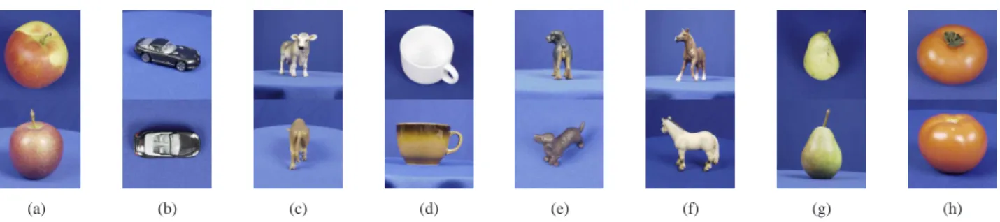
1) Datasets: The evaluations were conducted based on
two well-known datasets. The first dataset is the Caltech-4
dataset5. It is a composite of four different categories. They
are1074images of airplanes from the side,526images of cars
from the rear,826images of motorbikes from the side, and450
frontal face images from about 27 unique persons. Example
images from these four categories are shown in Fig. 7(a)-7(d).
The second dataset is the ETH-80 dataset 6 that consists of
eight categories: apple, car, cup, dog, pear, tomato, horse, and
cow. Each category has 410 images which are cropped, so
that they contain only the object in the center. Examples of
images from each category in the ETH-80dataset are shown
in Fig. 9. Our experiments were evaluated on the these two commonly used public datasets for the purpose of validating the effectiveness of the proposed method.
2) Descriptor Extraction: In recent years, many excellent
global and local descriptors have been proposed for the purpose of image categorization and object detection. For
5http://www.vision.caltech.edu/archive.html 6http://www.d2.mpi-inf.mpg.de/Datasets/ETH80 4 5 6 7 8 9 10 11 12 13 14 15 16 17 18 19 20 21 22 23 24 25 26 27 28 29 30 31 32 33 34 35 36 37 38 39 40 41 42 43 44 45 46 47 48 49 50 51 52 53 54 55 56 57 58 59 60
For Peer Review
(a) (b) (c) (d) (e) (f) (g) (h)
Fig. 9:Sample images from ETH-80dataset. (a) Apple. (b) Car. (c) Cow. (d) Cup. (e) Dog. (f) Horse. (g) Pear. (h) Tomato.
84 86 88 90 92 94 96
InIDMMSLB IDMMSLB InIDMMMCMC InGMM SVM
A cc u ra cy (i n % ) (a) Caltech-4 68 69 70 71 72 73 74 75 76
InIDMMSLB IDMMSLB InIDMMMCMC InGMM SVM
A cc u ra cy (i n % ) (b)ETH-80
Fig. 8: Boxplots for comparisons of the categorization accuracies’
distributions for the Caltech-4and the ETH-80datasets. The central
mark is the median, the edges of the box are the 25th
and 75th
percentiles. The outliers are marked individually.
example, the scale-invariant feature transform (SIFT) [57] descriptor, the local binary pattern (LBP) descriptor [58], and the Histogram of Oriented Gradient (HOG) descriptor [59]. The HOG descriptor, among others, has been one of the most popular and effective one for image categorization or detec-tion [60], [61]. In this paper, we employ the rectangular HOG (R-HOG) descriptor [62], an variant and improved version of HOG. With the principles of R-HOG and by considering seven windows and nine histogram bins, each image is represented
by a441-dimensional positive feature vector.
3) Image Categorization: Object categorization refers to
classifying a given image into a specific category, such as car, face, motorbike, and airplane. It can also be considered as an image categorization problem [63], which is an important and challenging problem in a wide range of application areas such as multimedia retrieval, pattern recognition and computer vision. Image categorization and its related applications have attracted considerable attention during the past few years [64]– [68]. The reason that image categorization has emerged as one
TABLE IV:Comparisons of object detections accuracies (in%) on
Caltech-4dataset. The standard deviations are in the brackets. Thep
-values of the student’s t-test with the null-hypothesis that InIDMMSLB
and the referring method have equal means but unknown variances are listed.
InIDMMSLB IDMMSLB InIDMMMCMC InGMM SVM
Airplanes 97.78 96.41 96.62 93.22 93.69 (0.78) (0.74) (0.75) (0.80) (0.79) p-value N/A 7.71×10⁻⁴ 0.0031 1.48×10−107.57×10⁻¹⁰ Faces 94.92 93.37 93.62 89.42 89.60 (0.56) (1.97) (0.98) (1.70) 0.65 p-value N/A 0.028 0.002 1.46×10−81.37×10−13 Cars 99.26 97.85 97.97 94.68 97.25 (0.64) (1.13) (0.82) (0.73) (0.68) p-value N/A 0.0029 9.57×10−41.28×10−112.31×10⁻⁶ Motorbikes 94.31 93.03 93.24 90.24 89.29 (0.63) (0.89) (0.77) (0.64) (0.83) p-value N/A 0.0017 0.0033 2.63×10−119.88×10⁻¹²
of the most active areas in the fields of image understanding and computer vision is mainly because its large potential in web image research, video retrieval, image database anno-tation, and medical image mining. Although human usually perform well on the task of image categorization, it remains difficult for computers to achieve similar performance. This is due to the various poses, different scales, multiple viewpoints. Our experiments for image categorization were implement-ed as follows. First, R-HOG descriptors were extractimplement-ed from each image. Each image in the datasets was then represented
by a 441-dimensional positive vector. Second, the vectors
from one category are assumed to be generated from an InIDMM. Each category has been randomly divided into equal training and test sets. For each category, one InIDMM was trained based on the training set. Third, the proposed Bayesian InIDMM was employed as a classifier to categorize objects by assigning the test image to a given class that has the highest posterior probability. Table III lists the average categorization
accuracies. It can be observed that the proposed InIDMMSLB
is superior to all the other referred methods. In order to
remove the randomness effect in the results, we conducted10
rounds of simulations and the mean values with the standard deviations are reported. The accuracy distributions are shown in Fig. 8.
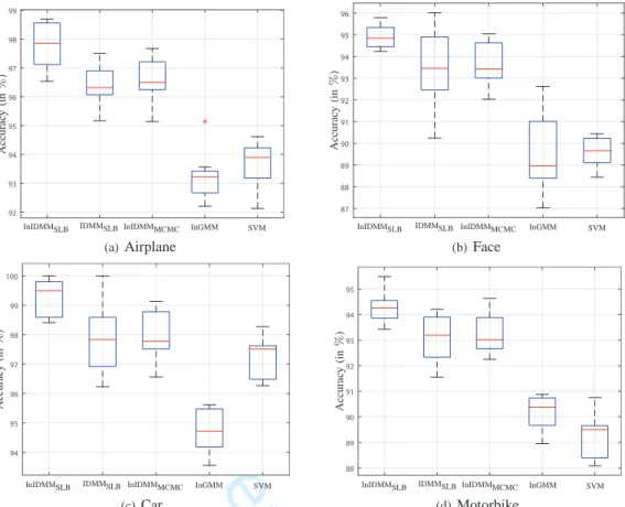
4) Object Detection: Object detection is another essential
problem in computer vision and has been commonly applied in various applications like content-based image retrieval, intelligent traffic management, driver assistance system, and video surveillance [69], [70]. The main goal of object detection is to find instances of real-world objects such as car, face, or bicycle in an images or a video clip. Typical object detec-tion algorithms apply the extracted features and employ the
6 7 8 9 10 11 12 13 14 15 16 17 18 19 20 21 22 23 24 25 26 27 28 29 30 31 32 33 34 35 36 37 38 39 40 41 42 43 44 45 46 47 48 49 50 51 52 53 54 55 56 57 58 59 60
For Peer Review
11 92 93 94 95 96 97 98 99InIDMMSLB IDMMSLB InIDMMMCMC InGMM SVM
A cc u ra cy (i n % ) (a)Airplane 87 88 89 90 91 92 93 94 95 96
InIDMMSLB IDMMSLB InIDMMMCMC InGMM SVM
A cc u ra cy (i n % ) (b)Face 94 95 96 97 98 99 100
InIDMMSLB IDMMSLB InIDMMMCMC InGMM SVM
A cc u ra cy (i n % ) (c)Car 88 89 90 91 92 93 94 95
InIDMMSLB IDMMSLB InIDMMMCMC InGMM SVM
A cc u ra cy (i n % ) (d)Motorbike
Fig. 10:Boxplots for comparisons of the detection accuracies’ distributions for the Caltech-4. The central mark is the median, the edges of
the box are the25th
and75th
percentiles. The outliers are marked individually. learning algorithms to recognize the instances from an object
class. Here, we apply the proposed InIDMM as a classifier and study its performance in object detection. Similar as image categorization, we also applied the R-HOG descriptor to represent an image. Each image in the dataset was represented
by a441-dimensional positive feature vector.
For the experiments on the Caltech-4dataset, we evaluated
the detection performance on the four sub-datasets mentioned in Sec. IV-B3. In addition these four datasets, we used the
Caltech background sub-dataset (451 images) as the
non-object sub-dataset for these four non-object sub-classes. Samples images from each of these four object classes and the Caltech background dataset are shown in Fig 7.
The proposed InIDMM is utilized as a classifier to detect the objects through assigning the testing image to a given group (object or non-object). Table IV summarizes the detection accuracies. It can be observed from these results that the InIDMM provides the best detection accuracies compared to the other methods. During the evaluations, each of the aforementioned sub-datasets were randomly into two separate halves, one for training and the other one for test. Ten rounds of simulations were conducted and the mean values with the standard deviations are reported. Figure 10 illustrates the distributions of the detection accuracies.
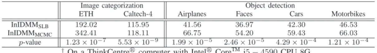
5) Computational efficiency: As emphasized at the
intro-duction section of this paper, one motivation of applying the EVI framework to derive analytically tractable solution for InIDMM such that the computational cost can be reduced, compared with numerical solution. In Tab. V, we compare
the required runtime for InIDMMSLB and InIDMMMCMC.
Ten rounds of simulations were conducted and the mean
values are reported. Thep-values of the student’s t-test with
the null-hypothesis that the runtimes of InIDMMSLB and
InIDMMMCMC have equal means but unknown variances are
listed.It can be concluded that the proposed InIDMMSLB has
statistically significantly superior performance in terms of runtime.
V. CONCLUSIONS
The inverted Dirichlet distribution has been widely applied in modeling the positive vector (vector that contains only positive elements). The Dirichlet processing mixture of the inverted Dirichlet mixture model (InIDMM) can provide good modeling performance to the positive vectors. Compared to the conventional finite inverted Dirichlet mixture model (IDMM), the InIDMM has more flexible model complexity as the number of mixture components can be automatically deter-mined. Moreover, the over-fitting and under-fitting problem is avoided by the Bayesian estimation of InIDMM. To obtain an analytically tractable solution for Bayesian estimation of InID-MM, we utilized the recently proposed extended variational inference (EVI) framework. With single lower bound (SLB) approximation, the convergence of the proposed analytically tractable solution is guaranteed, while the solution obtained via multiple lower bound (MLB) approximations may result in oscillations of the objective function. Extensive synthesized data evaluations and real data evaluations demonstrated the superior performance of the proposed method.
REFERENCES
[1] B. Everitt and D. Hand, Finite Mixture Distributions. Chapman and Hall, London, UK, 1981.
4 5 6 7 8 9 10 11 12 13 14 15 16 17 18 19 20 21 22 23 24 25 26 27 28 29 30 31 32 33 34 35 36 37 38 39 40 41 42 43 44 45 46 47 48 49 50 51 52 53 54 55 56 57 58 59 60
For Peer Review
TABLE V:Comparisons of runtime (ins)†for InIDMMSLB and InIDMMMCMC.
Image categorization Object detection
ETH Caltech-4 Airplanes Faces Cars Motorbikes
InIDMMSLB 192.02 115.95 41.56 36.97 42.30 46.53
InIDMMMCMC 342.41 118.11 66.75 54.20 59.43 66.03
p-value 1.23×10⁻⁷ 5.53×10⁻⁹ 1.99×10⁻⁵ 2.46×10⁻⁵ 4.29×10⁻⁴ 1.21×10⁻⁴
†On a ThinkCentrer
computer with IntelrCoreTM i5−4590CPU8G.
[2] C. M. Bishop, Pattern Recognition and Machine Learning (Information
Science and Statistics). Springer-Verlag New York, Inc., 2006. [3] N. Bouguila, D. Ziou, and J. Vaillancourt, “Unsupervised learning
of a finite mixture model based on the Dirichlet distribution and its application,” IEEE Transactions on Image Processing, vol. 13, no. 11, pp. 1533–1543, 2004.
[4] S. Bram, “Modeling and analysis of wireless channels via the mixture of Gaussian distribution,” vol. 65, no. 3, pp. 951–957, 2015.
[5] Z. Ma, A. E. Teschendorff, A. Leijon, Y. Qiao, H. Zhang, and J. Guo, “Variational Bayesian matrix factorization for bounded support da-ta,” IEEE Transactions on Pattern Analysis and Machine Intelligence, vol. 37, no. 4, pp. 876–89, 2015.
[6] Z. Ma, P. K. Rana, J. Taghia, M. Flierl, and A. Leijon, “Bayesian esti-mation of Dirichlet mixture model with variational inference,” Pattern
Recognition, vol. 47, no. 9, pp. 3143–3157, 2014.
[7] Z. Ma and A. Leijon, “Bayesian estimation of beta mixture models with variational inference.” IEEE Transactions on Pattern Analysis and
Machine Intelligence, vol. 33, no. 11, pp. 2160–73, 2011.
[8] D. A. Reynolds and R. C. Rose, “Robust text-independent speaker iden-tification using Gaussian mixture speaker models,” IEEE Transactions
on Speech and Audio Processing, vol. 3, no. 1, pp. 72–83, 1995.
[9] N. Nasios and A. G. Bors, “Variational learning for Gaussian mixture models,” IEEE Transactions on Systems Man and Cybernetics Part B
(Cybernetics), vol. 36, no. 4, pp. 849–862, July 2006.
[10] S. Sun and X. Xu, “Variational inference for infinite mixtures of Gaussian processes with applications to traffic flow prediction,” IEEE
Transactions on Intelligent Transportation Systems, vol. 12, no. 2, pp.
466–475, June 2011.
[11] J. Jung, S. R. Lee, H. Park, S. Lee, and I. Lee, “Capacity and error probability analysis of diversity reception schemes over generalized-K
fading channels using a mixture gamma distribution,” IEEE Transactions
on Wireless Communications, vol. 13, no. 9, pp. 4721–4730, Sept 2014.
[12] J. Taghia, Z. Ma, and A. Leijon, “Bayesian estimation of the von-Mises Fisher mixture model with variational inference,” IEEE Transactions on
Pattern Analysis and Machine Intelligence, vol. 36, no. 9, pp. 1701–
1715, Sept 2014.
[13] E. A. Houseman, B. C. Christensen, R. F. Yeh, C. J. Marsit, M. R. Kara-gas, M. Wrensch, H. H. Nelson, J. Wiemels, S. Zheng, J. K. Wiencke, and K. T. Kelsey, “Model-based clustering of DNA methylation array data: a recursive-partitioning algorithm for high-dimensional data arising as a mixture of beta distributions,” Bioinformatics, vol. 9, p. 365, 2008. [14] J. M. P. Nascimento and J. M. Bioucas-Dias, “Hyperspectral unmixing based on mixtures of Dirichlet components,” IEEE Transactions on
Geoscience and Remote Sensing, vol. 50, no. 3, pp. 863–878, March
2012.
[15] Q. He, K. Chang, E. P. Lim, and A. Banerjee, “Keep it simple with time: A reexamination of probabilistic topic detection models,” IEEE
Transactions on Pattern Analysis and Machine Intelligence, vol. 32,
no. 10, pp. 1795–1808, Oct 2010.
[16] T. Bdiri and N. Bouguila, “Positive vectors clustering using inverted Dirichlet finite mixture models,” Expert Systems with Applications, vol. 39, no. 2, pp. 1869–1882, 2012.
[17] ——, “Bayesian learning of inverted Dirichlet mixtures for SVM kernels generation,” Neural Computing and Applications, vol. 23, no. 5, pp. 1443–1458, 2013.
[18] P. O. Hoyer, “Non-negative matrix factorization with sparseness con-straints,” The Journal of Machine Learning Research, vol. 5, no. 11, pp. 1457–1469, Nov. 2004.
[19] S. C. Markley and D. J. Miller, “Joint parsimonious modeling and model order selection for multivariate Gaussian mixtures,” IEEE Journal of
Selected Topics in Signal Processing, vol. 4, no. 3, pp. 548–559, June
2010.
[20] Z. Liang and S. Wang, “An EM approach to MAP solution of segmenting tissue mixtures: a numerical analysis.” IEEE Transactions on Medical
Imaging, vol. 28, no. 2, pp. 297–310, 2009.
[21] N. Bouguila and D. Ziou, “Unsupervised selection of a finite Dirich-let mixture model: an MML-based approach,” IEEE Transactions on
Knowledge and Data Engineering, vol. 18, no. 8, pp. 993–1009, June
2006.
[22] S. Richardson and P. J. Green, “Corrigendum: On bayesian analysis of mixtures with an unknown number of components,” Journal of the Royal
Statistical Society, vol. 60, no. 3, p. 661, 1996.
[23] S. Sun, “A review of deterministic approximate inference techniques for Bayesian machine learning,” Neural Computing and Applications, vol. 23, no. 7-8, pp. 2039–2050, Dec. 2013.
[24] L. Huang, Y. Xiao, K. Liu, H. C. So, and J. K. Zhang, “Bayesian information criterion for source enumeration in large-scale adaptive antenna array,” IEEE Transactions on Vehicular Technology, vol. 65, no. 5, pp. 3018–3032, May 2016.
[25] X. Chen, “Using Akaike information criterion for selecting the field distribution in a reverberation chamber,” IEEE Transactions on
Electro-magnetic Compatibility, vol. 55, no. 4, pp. 664–670, Aug 2013.
[26] K. Bousmalis, S. Zafeiriou, L. P. Morency, M. Pantic, and Z. Ghahra-mani, “Variational infinite hidden conditional random fields,” IEEE
Transactions on Pattern Analysis and Machine Intelligence, vol. 37,
no. 9, pp. 1917–1929, Sept 2015.
[27] M. Meilˇa and H. Chen, “Bayesian non-parametric clustering of ranking data,” IEEE Transactions on Pattern Analysis and Machine Intelligence, vol. 38, no. 11, pp. 2156–2169, Nov 2016.
[28] Y. Xu, M. Megjhani, K. Trett, W. Shain, B. Roysam, and Z. Han, “Un-supervised profiling of microglial arbor morphologies and distribution using a nonparametric Bayesian approach,” IEEE Journal of Selected
Topics in Signal Processing, vol. 10, no. 1, pp. 115–129, Feb 2016.
[29] T. S. Ferguson, “A Bayesian analysis of some nonparametric problems,”
Annals of Statistics, vol. 1, no. 2, pp. 209–230, 1973.
[30] C. E. Antoniak, “Mixtures of Dirichlet processes with applications to Bayesian nonparametric problems,” Annals of Statistics, vol. 2, no. 6, pp. 1152–1174, 1974.
[31] N. L. Hjort, C. Holmes, P. M¨uller, and S. G. Walker, Eds., Bayesian
Nonparametrics. Cambridge University Press, 2010.
[32] Y. W. Teh and D. M. Blei, “Hierarchical Dirichlet processes,” Journal of
the American Statistical Association, vol. 101, no. 476, pp. 1566–1581,
2006.
[33] N. J. Foti and S. A. Williamson, “A survey of non-exchangeable priors for Bayesian nonparametric models,” IEEE Transactions on Pattern
Analysis and Machine Intelligence, vol. 37, no. 2, pp. 359–371, Feb
2015.
[34] W. Fan and N. Bouguila, “Online learning of a Dirichlet process mixture of beta-Liouville distributions via variational inference,” IEEE
Transactions on Neural Networks and Learning Systems, vol. 24, no. 11,
pp. 1850–1862, 2013.
[35] X. Wei and C. Li, “The infinite student’s t -mixture for robust modeling,”
Signal Processing, vol. 92, no. 1, pp. 224–234, 2012.
[36] N. Bouguila and D. Ziou, “A Dirichlet process mixture of generalized Dirichlet distributions for proportional data modeling,” IEEE
Transac-tions on Neural Networks, vol. 21, no. 1, pp. 107–122, 2010.
[37] X. Wei and Z. Yang, “The infinite student’s t -factor mixture analyzer for robust clustering and classification ,” Pattern Recognition, vol. 45, no. 12, pp. 4346–4357, 2012.
[38] S. P. Chatzis and G. Tsechpenakis, “The infinite hidden Markov random field model.” IEEE Transactions on Neural Networks, vol. 21, no. 6, pp. 1004–14, 2010.
[39] M. Wedel and P. Lenk, Markov Chain Monte Carlo. Boston, MA: Springer US, 2013, pp. 925–930.
[40] M. Pereyra, P. Schniter, E. Chouzenoux, J. C. Pesquet, J. Y. Tourneret, A. O. Hero, and S. McLaughlin, “A survey of stochastic simulation and optimization methods in signal processing,” IEEE Journal of Selected
Topics in Signal Processing, vol. 10, no. 2, pp. 224–241, Mar. 2016.
[41] M. I. Jordan, Z. Ghahramani, T. S. Jaakkola, and L. K. Saul, “An introduction to variational methods for graphical models,” Machine
Learning, vol. 37, no. 2, pp. 183–233, 1999.
[42] J. Taghia and A. Leijon, “Variational inference for Watson mixture mod-el,” IEEE Transactions on Pattern Analysis and Machine Intelligence, vol. 38, no. 9, pp. 1886–1900, 2015. 6 7 8 9 10 11 12 13 14 15 16 17 18 19 20 21 22 23 24 25 26 27 28 29 30 31 32 33 34 35 36 37 38 39 40 41 42 43 44 45 46 47 48 49 50 51 52 53 54 55 56 57 58 59 60