Foundations and Advances in Deep Learning

(1)

9HSTF

MG*aff

hej+

ISBN 978-952-60-5574-9 ISBN 978-952-60-5575-6 (pdf) ISSN-L 1799-4934 ISSN 1799-4934 ISSN 1799-4942 (pdf) Aalto University School of Science Department of Information and Computer Science www.aalto.fi BUSINESS + ECONOMY ART + DESIGN + ARCHITECTURE SCIENCE + TECHNOLOGY CROSSOVER DOCTORAL A a lto -D D 2 1 /2 0 1 4 K yu ng hy un C ho Fo un da tio ns an d A dv an ce s in D ee p L ea rn in g A a lt o U n iv e rs it y

Foundations and Advances

in Deep Learning

K

y

ung

h

y

un C

h

o

DOCTORAL DISSERTATIONS

(2)

Aalto University publication series DOCTORAL DISSERTATIONS 21/2014

Foundations and Advances

in Deep Learning

Kyunghyun Cho

A doctoral dissertation completed for the degree of Doctor of Science (Technology) to be defended, with the permission of the Aalto University School of Science, at a public examination held at the lecture hall T2 of the school on 21 March 2014 at 12.

Aalto University School of Science

(3)

Prof. Juha Karhunen Thesis advisor

Prof. Tapani Raiko and Dr. Alexander Ilin Preliminary examiners

Prof. Hugo Larochelle, University of Sherbrooke, Canada Dr. James Bergstra, University of Waterloo, Canada Opponent

Prof. Nando de Freitas, University of Oxford, United Kingdom

Aalto University publication series DOCTORAL DISSERTATIONS 21/2014 © Kyunghyun Cho ISBN 978-952-60-5574-9 ISBN 978-952-60-5575-6 (pdf) ISSN-L 1799-4934 ISSN 1799-4934 (printed) ISSN 1799-4942 (pdf) http://urn.fi/URN:ISBN:978-952-60-5575-6 Unigrafia Oy Helsinki 2014

(4)

Abstract

Aalto University, P.O. Box 11000, FI-00076 Aalto www.aalto.fi

Author Kyunghyun Cho

Name of the doctoral dissertation Foundations and Advances in Deep Learning Publisher

Unit Department of Information and Computer Science

Series Aalto University publication series DOCTORAL DISSERTATIONS 21/2014 Field of research Machine Learning

Manuscript submitted 2 September 2013 Date of the defence 21 March 2014 Permission to publish granted (date) 7 January 2014 Language English Monograph Article dissertation (summary + original articles) Abstract

Deep neural networks have become increasingly popular under the name of deep learning recently due to their success in challenging machine learning tasks. Although the popularity is mainly due to recent successes, the history of neural networks goes as far back as 1958 when Rosenblatt presented a perceptron learning algorithm. Since then, various kinds of artiﬁcial neural networks have been proposed. They include Hopﬁeld networks, self-organizing maps, neural principal component analysis, Boltzmann machines, multi-layer perceptrons, radial-basis function networks, autoencoders, sigmoid belief networks, support vector machines and deep belief networks.

The first part of this thesis investigates shallow and deep neural networks in search of principles that explain why deep neural networks work so well across a range of applications. The thesis starts from some of the earlier ideas and models in the field of artificial neural networks and arrive at autoencoders and Boltzmann machines which are two most widely studied neural networks these days. The author thoroughly discusses how those various neural networks are related to each other and how the principles behind those networks form a foundation for autoencoders and Boltzmann machines.

The second part is the collection of the ten recent publications by the author. These publications mainly focus on learning and inference algorithms of Boltzmann machines and autoencoders. Especially, Boltzmann machines, which are known to be difﬁcult to train, have been in the main focus. Throughout several publications the author and the co-authors have devised and proposed a new set of learning algorithms which includes the enhanced gradient, adaptive learning rate and parallel tempering. These algorithms are further applied to a restricted Boltzmann machine with Gaussian visible units.

In addition to these algorithms for restricted Boltzmann machines the author proposed a two-stage pretraining algorithm that initializes the parameters of a deep Boltzmann machine to match the variational posterior distribution of a similarly structured deep autoencoder. Finally, deep neural networks are applied to image denoising and speech recognition.

Keywords Deep Learning, Neural Networks, Multilayer Perceptron, Probabilistic Model, Restricted Boltzmann Machine, Deep Boltzmann Machine, Denoising Autoencoder ISBN (printed) 978-952-60-5574-9 ISBN (pdf) 978-952-60-5575-6

ISSN-L 1799-4934 ISSN (printed) 1799-4934 ISSN (pdf) 1799-4942 Location of publisher Helsinki Location of printing Helsinki Year 2014

(5)

(6)

Preface

This dissertation summarizes the work I have carried out as a doctoral student at the Department of Information and Computer Science, Aalto University School of Science under the supervision of Prof. Juha Karhunen, Prof. Tapani Raiko and Dr. Alexander Ilin between 2011 and early 2014, while being generously funded by the Finnish Doctoral Programme in Computational Sciences (FICS). None of these had been possible without enormous support and help from my supervisors, the depart-ment and the Aalto University. Although I cannot express my gratitude fully in words, let me try: Thank you!

During these years I was a part of a group which started as a group onBayesian Modelingled by Prof. Karhunen, but recently become a group onDeep Learning and Bayesian Modelingco-led by Prof. Karhunen and Prof. Raiko. I would like to thank all the current members of the group: Prof. Karhunen, Prof. Raiko, Dr. Ilin, Mathias Berglund and Jaakko Luttinen.

I have spent most of my doctoral years at the Department of Information and Computer Science and have been lucky to have collaborated and discussed with researchers from other groups on interesting topics. I thank Xi Chen, Konstanti-nos Georgatzis (University of Edinburgh), Mark van Heeswijk, Sami Keronen, Dr. AmauryMomoLendasse, Dr. Kalle Palomäki, Dr. Nima Reyhani (Valo Research and Trading), Dusan Sovilj, Tommi Suvitaival and Seppo Virtanen (of course, not in the order of preference, but in the alphabetical order). Unfortunately, due to the space restriction I cannot list all the colleagues, but I would like to thank all the others from the department as well.Kiitos!

I was warmly invited by Prof. Yoshua Bengio to Laboratoire d’Informatique des Systèmes Adaptatifs (LISA) at the Université de Montréal for six months (Aug. 2013 – Jan. 2014). I ﬁrst must thank FICS for kindly funding the research visit so that I had no worry about daily survival. The visit at the LISA was fun and productive! Although I would like to list all of the members of the LISA to show my apprecia-tion during my visit, I can only list a few: Guillaume Allain, Frederic Bastien, Prof.

(7)

Bengio, Prof. Aaron Courville, Yann Dauphin, Guillaume Desjardins (Google Deep-Mind), Ian Goodfellow, Caglar Gulcehre, Pascal Lamblin, Mehdi Mirza, Razvan Pas-canu, David Warde-Farley and Li Yao (again, in the alphabetical order). Remember, it is Yoshua, not me, who recruited so many students.Merci!

Outside my comfort zones, I would like to thank Prof. Sven Behnke (University of Bonn, Germany), Prof. Hal Daumé III (University of Maryland), Dr. Guido Montú-far (Max Planck Institute for Mathematics in the Sciences, Germany), Dr. Andreas Müller (Amazon), Hannes Schulz (University of Bonn) and Prof. Holger Schwenk (Université du Maine, France) (again, in the alphabetical order).

I express my gratitude to Prof. Nando de Freitas of the University of Oxford, the opponent in my defense. I would like to thank the pre-examiners of the disserta-tion; Prof. Hugo Larochelle of the University of Sherbrooke, Canada and Dr. James Bergstra of the University of Waterloo, Canada for their valuable and thorough com-ments on the dissertation.

I have spent half of my twenties in Finland from Summer, 2009 to Spring, 2014. Those five years have been delightful and ex-citing both academically and personally. Living and studying in Finland have impacted me so significantly and positively that I cannot imagine myself without these five years. I thank all the people I have met in Finland and the country in general for

hav-ing given me this enormous opportunity. Without any surprise, I must express my gratitude toAlkofor properly regulating the sales of alcoholic beverages in Finland.

Again, I cannot list all the friends I have met here in Finland, but let me try to thank at least a few: Byungjin Cho (and his wife), Eunah Cho, Sungin Cho (and his girlfriend), Dong UkTerryLee, Wonjae Kim, InseopLeoLee, Seunghoe Roh, Marika Pasanen (and her boyfriend), Zaur Izzadust, Alexander Grigorievsky (and his wife), David Padilla, Yu Shen, Roberto Calandra, Dexter He and Anni Rautanen (and her boyfriend and family) (this time, in a random order).Kiitos!

I thank my parents for their enormous support. I thankandcongratulate my little brother who married a beautiful woman who recently gave a birth to a beautiful baby. Lastly but certainly not least, my gratitude and love goes toY. Her encouragement and love have kept me and my research sane throughout my doctoral years.

Espoo, February 17, 2014,

(8)

List of Publications

This thesis consists of an overview and of the following publications which are re-ferred to in the text by their Roman numerals.

I Kyunghyun Cho, Tapani Raiko and Alexander Ilin. Enhanced Gradient for Training Restricted Boltzmann Machines. Neural Computation, Volume 25 Issue 3 Pages 805–831, March 2013.

IIKyunghyun Cho, Tapani Raiko and Alexander Ilin. Enhanced Gradient and Adap-tive Learning Rate for Training Restricted Boltzmann Machines. InProceedings of the 28th International Conference on Machine Learning (ICML 2011), Pages 105–112, June 2011.

IIIKyunghyun Cho, Tapani Raiko and Alexander Ilin. Parallel Tempering is Ef-ﬁcient for Learning Restricted Boltzmann Machines. InProceedings of the 2010 International Joint Conference on Neural Networks (IJCNN 2010), Pages 1–8, July 2010.

IV Kyunghyun Cho, Alexander Ilin and Tapani Raiko. Tikhonov-Type Regulariza-tion for Restricted Boltzmann Machines. InProceedings of the 22nd International Conference on Artiﬁcial Neural Networks (ICANN 2012), Pages 81–88, September 2012.

VKyunghyun Cho, Alexander Ilin and Tapani Raiko. Improved Learning of Gaussian-Bernoulli Restricted Boltzmann Machines. InProceedings of the 21st International Conference on Artiﬁcial Neural Networks (ICANN 2011), Pages 10–17, June 2011.

(13)

VI Kyunghyun Cho, Tapani Raiko and Alexander Ilin. Gaussian-Bernoulli Deep Boltzmann Machines. InProceedings of the 2013 International Joint Conference on Neural Networks (IJCNN 2013), August 2013.

VIIKyunghyun Cho, Tapani Raiko, Alexander Ilin and Juha Karhunen. A Two-Stage Pretraining Algorithm for Deep Boltzmann Machines. InProceedings of the 23rd International Conference on Artiﬁcial Neural Networks (ICANN 2013), Pages 106–113, September 2013.

VIIIKyunghyun Cho. Simple Sparsiﬁcation Improves Sparse Denoising Autoen-coders in Denoising Highly Corrupted Images. InProceedings of the 30th Interna-tional Conference on Machine Learning (ICML 2013), Pages 432–440, June 2013.

IX Kyunghyun Cho. Boltzmann Machines for Image Denoising. InProceedings of the 23rd International Conference on Artiﬁcial Neural Networks (ICANN 2013), Pages 611–618, September 2013.

XSami Keronen, Kyunghyun Cho, Tapani Raiko, Alexander Ilin and Kalle Palomäki. Gaussian-Bernoulli Restricted Boltzmann Machines and Automatic Feature Ex-traction for Noise Robust Missing Data Mask Estimation. InProceedings of the 38th International Conference on Acoustics, Speech, and Signal Processing (ICASSP 2013), Pages 6729–6733, May 2013.

(14)

List of Abbreviations

BM Boltzmann machine CD Contrastive divergence DBM Deep Boltzmann machine DBN Deep belief network DEM Deep energy model ELM Extreme learning machine EM Expectation-Maximization

GDBM Gaussian-Bernoulli deep Boltzmann machine GP Gaussian Process

GP-LVM Gaussian process latent variable model

GRBM Gaussian-Bernoulli restricted Boltzmann machine ICA Independent component analysis

KL Kullback-Leibler divergence

lasso Least absolute shrinkage and selection operator MAP Maximum-a-posteriori estimation

MCMC Markov Chain Monte Carlo MLP Multilayer perceptron MoG Mixture of Gaussians MRF Markov random ﬁeld OMP Orthogonal matching pursuit PCA Principal component analysis PoE Product of Experts

PSD Predictive sparse decomposition RBM Restricted Boltzmann machine SESM Sparse encoding symmetric machine SVM Support vector machine

(15)

(16)

Mathematical Notation

As the author has tried to make mathematical notations consistent throughout this thesis, in some parts they may look different from how they are used commonly in the original research literature. Before entering the main text of the thesis, the author would like to declare and clarify the mathematical notations which will be used repeatedly.

Variables and Parameters

A vector, which is always assumed to be a column vector, is mostly denoted by a bold, lower-case Roman letter such asx, and a matrix by a bold, upper-case Roman letter such asW. Two important exceptions areθandμwhich denote a vector of parameters and a vector of variational parameters, respectively.

A component of a vector is denoted by a (non-bold) lower-case Roman letter with the index of the component as a subscript. Similarly, an element of a matrix is denoted by a (non-bold) lower-case Roman letter with a pair of the indices of the component as a subscript. For instance,xiandwij indicate thei-th component of xand the

element ofWon itsi-th row andj-th column, respectively.

Lower-case Greek letters are used, in most cases, to denote scalar variables and parameters. For instance,η,λandσmean learning rate, regularization constant and standard deviation, respectively.

Functions

Regardless of the type of its output, all functions are denoted by non-bold letters. In the case of vector functions, the dimensions of the input and output will be explicitly explained in the text, unless they are obvious from the context. Similarly to a vector notation, a subscript may be used to denote a component of a vector function such thatfi(x)is thei-th component of a vector functionf.

(17)

Some commonly used functions include a component-wise nonlinear activation functionφ, a stochastic noise operatorκ, an encoder functionf, and a decoder func-tiong.

A component-wise nonlinear activation functionφis used for different types of ac-tivation functions depending on the context. For instance,φis a Heaviside function (see Eq. (2.5)) when used in a Hopﬁeld network, but is a logistic sigmoid function (see Eq. (2.7)) in the case of Boltzmann machines. There should not be any confu-sion, as its deﬁnition will always be explicitly given at each usage.

Probability and Distribution

A probability density/mass function is often denoted byporPand the corresponding unnormalized probability byp∗orP∗. By dividingp∗by the normalization constant

Z, one recoversp. Additionally,q orQare often used to denote a (approximate) posterior distribution over hidden or latent variables.

An expectation of a functionf(x)over a distributionpis denoted either byEp[f(x)]

or byf(x)_p. A cross-covariance of two random vectorsxandyover probability densitypis often denoted byCovp(x,y). KL(QP)means a Kullback-Leibler

di-vergence (see Eq. (2.26)) between distributionsQandP.

Two important types of distributions that will be used throughout this thesis are the data distribution and the model distribution. The data distribution is the distribution from which training samples are sampled, and the model distribution is the one that is represented by a machine learning model. For instance, a Boltzmann machine deﬁnes a distribution over all possible states of visible units, and that distribution is referred to as the model distribution.

The data distribution is denoted by either d,pDorP0, and the model distribution

by either m,porP_∞. Reasons for using different notations for the same distribution will be made clear throughout the text.

Superscripts and Subscripts

In machine learning, it is usually either explicitly or implicitly assumed that a set of training samples are given.Nis often used to denote the size of the training set, and each sample is denoted by its index in the super- or subscript such thatx(n)is the

n-th training sample. However, as it is aset, it should be understood that the order of the elements is arbitrary.

(18)

Then we use either a superscript or subscript to indicate the layer to which each unit or a vector of units belongs. For instance,h[l]andW[l]are respectively a vector of (hidden) units and a matrix of weight parameters in thel-th layer. Whenever it is necessary to make an equation less cluttered,h[l] (superscript) andh_[l] (subscript)

may be used interchangeably.

Occasionally, there appears an ordered sequence of variables or parameters. In that case, a super- or subscripttis used to denote the temporal index of a variable. For example, bothxtandxtmean thet-th vectorxor the value of a vectorxat time t.

The latter two notations[l]andtapply also to functions as well as probability density/mass functions. For instance,f[l]is an encoder function that projects units in thel-th layer to the(l+ 1)-th layer. In the context of Markov Chain Monte Carlo sampling,ptdenotes a probability distribution over the states of a Markov chain aftertsteps of simulation.

In many cases,θ∗andθˆdenote an unknown optimal value and a value estimated by, say, an optimization algorithm, respectively. However, one should be aware that these notations are not strictly followed in some parts of the text. For example,x∗

(19)

(20)

1. Introduction

1.1 Aim of this Thesis

A research field, calleddeep learning, has gained its popularity recently as a way of learning deep, hierarchical artificial neural networks (see, for example, Bengio, 2009). Especially, deep neural networks such as a deep belief network (Hinton et al., 2006), deep Boltzmann machine (Salakhutdinov and Hinton, 2009a), stacked denois-ing autoencoders (Vincent et al., 2010) and many other variants have been applied to various machine learning tasks with impressive improvements over conventional approaches. For instance, Krizhevsky et al. (2012) significantly outperformed all other conventional methods in classifying a huge set of large images. Speech recog-nition also benefited significantly by using a deep neural network recently (Hinton et al., 2012). Also, many other tasks such as traffic sign classification (Ciresan et al., 2012c) have been shown to benefit from using a large, deep neural network.

Although the recent surge of popularity stems from the introduction of layer-wise pretraining proposed in 2006 by Hinton and Salakhutdinov (2006); Bengio et al. (2007); Ranzato et al. (2007b), research on artificial neural networks began as early as 1958 when Rosenblatt (1958) presented the first perceptron learning algorithm. Since then, various kinds of artificial neural networks have been proposed. They include, but are not limited to Hopfield networks (Hopfield, 1982), self-organizing maps (Ko-honen, 1982), neural networks for principal component analysis (Oja, 1982), Boltz-mann machines (Ackley et al., 1985), multilayer perceptrons (Rumelhart et al., 1986), radial-basis function networks (Broomhead and Lowe, 1988), autoencoders (Baldi and Hornik, 1989), sigmoid belief networks (Neal, 1992) and support vector ma-chines (Cortes and Vapnik, 1995).

These types of artiﬁcial neural networks are interesting not only on their own, but by connections among themselves and with other machine learning approaches. For instance, principal component analysis (PCA) which may be considered a linear

(21)

alge-braic method, arises also from an unsupervised neural network with Oja’s rule (Oja, 1982), and at the same time, can be recovered from a latent variable model (Tipping and Bishop, 1999; Roweis, 1998). Also, the cost function used to train a linear au-toencoder with a single hidden layer corresponds exactly to that of PCA. PCA can be further generalized to nonlinear PCA through, for instance, an autoencoder with multiple nonlinear hidden layers (Kramer, 1991; Oja, 1991).

Due to the recent popularity of deep learning, two of the most widely studied ar-tiﬁcial neural networks are autoencoders and Boltzmann machines. An autoencoder with a single hidden layer as well as a structurally restricted version of the Boltzmann machine, called a restricted Boltzmann machine, have become popular due to their application in layer-wise pretraining of deep multilayer perceptrons.

Thus, this thesis starts from some of the earlier ideas in the artificial neural net-works and arrives at those two currently popular models. In due course, the author will explain how various types of artificial neural networks are related to each other, ultimately leading to autoencoders and Boltzmann machines. Furthermore, this the-sis will include underlying methods and concepts that have led to those two models’ popularity, which include, for instance, layer-wise pretraining and manifold learn-ing. Whenever it is possible, informal mathematical justification for each model or method is provided alongside.

Since the main focus of this thesis is ongeneralprinciples of deep neural networks, the thesis avoids describing any method that is speciﬁc to a certain task. In other words, the explanations as well as the models in this thesis assume no prior knowl-edge about data, except that each sample is independent and identically distributed and that its length is ﬁxed.

Ultimately, the author hopes that the reader, even without much background on deep learning, will understand the basic principles and concepts of deep neural net-works.

1.2 Outline

This dissertation aims to provide an introduction to deep neural networks throughout which the author’s contributions are placed. Starting from simple neural networks that were introduced as early as 1958, we gradually move toward the recent advances in deep neural networks.

For clarity, contributions that have been proposed and presented by the author are emphasized with bold-face. A separate list of the author’s contributions is given in Section 1.3.

(22)

1.2.1 Shallow Neural Networks

In Chapter 2, the author gives a background on neural networks that are considered shallow. By shallow neural networks we refer, in the case of supervised models, to those neural networks that have only input and output units, although many often consider a neural network having a single layer of hidden units shallow as well. No intermediate hidden units are considered. A linear regression network and perceptron are described as representative examples of supervised, shallow neural networks in Section 2.1.

Unsupervised neural networks which do not have any output unit are considered shallow when either there are no hidden units or there are only linear hidden units. A Hopﬁeld network is one example having no hidden units, and a linear autoencoder, or equivalently principal component analysis, is an example having linear hidden units only. Both of them are brieﬂy described in Section 2.2.

All these shallow neural networks are then in Section 2.3 further described in rela-tion with probabilistic models. From this probabilistic perspective, the computarela-tions in neural networks are interpreted as computing the conditional probability of other units given an input sample. In supervised neural networks, these forward computa-tions correspond to computing the conditional probability of output variables, while in unsupervised neural networks, they are shown to be equivalent to inferring the posterior distribution of hidden units under certain assumptions.

Based on this preliminary knowledge on shallow neural networks, the author dis-cusses some conditions that are often satisﬁed by a neural network to be considered deep in Section 2.4.

The chapter ends by brieﬂy describing how the parameters of a neural network can be efﬁciently estimated by the stochastic gradient method.

1.2.2 Deep Feedforward Neural Networks

The ﬁrst family of deep neural networks is introduced and discussed in detail in Chap-ter 3. This family consists of feedforward neural networks that have multiple layers of nonlinear hidden units. A multilayer perceptron is introduced and two related, but not-so-deep, feedforward neural networks, a kernel support vector machine and an extreme learning machine are brieﬂy discussed in Section 3.1.

The remaining part of the chapter begins by describing deep autoencoders. With its basic description, a probabilistic interpretation of the encoder and decoder of a deep autoencoder is provided in connection with a sigmoid belief network and its learning algorithm called wake-sleep algorithm in Section 3.2.1. This allows one to view the encoder and decoder as inferring an approximate posterior distribution

(23)

and computing a conditional distribution. Under this view, a related approach called sparse coding is discussed, and anexplicit sparsiﬁcation, proposed by the author in Publication VIII, for a sparse deep autoencoder is introduced in Section 3.2.5.

Another view of an autoencoder is provided afterward based on the manifold as-sumption in Section 3.3. In this view, it is explained how some variants of autoen-coders such as a denoising autoencoder and a contractive autoencoder are able to capture the manifold on which data lies.

An algorithm called backpropagation for efﬁciently computing the gradient of the cost function of a feedforward neural network with respect to the parameters is pre-sented in Section 3.4. The computed gradient is often used by the stochastic gradient method to estimate the parameters.

After a brief description of backpropagation, the section further discusses the dif-ﬁculty of training deep feedforward neural networks by introducing some of the hy-potheses proposed recently. Furthermore, for each hypothesis, a potential remedy is described.

1.2.3 Boltzmann Machines with Hidden Units

The second family of deep neural networks considered in this dissertation consists of a Boltzmann machine and its structurally restricted variants. The author classiﬁes the Boltzmann machines as deep neural networks based on the observation that Boltz-mann machines are recurrent neural networks and that any recurrent neural network with nonlinear hidden units is deep.

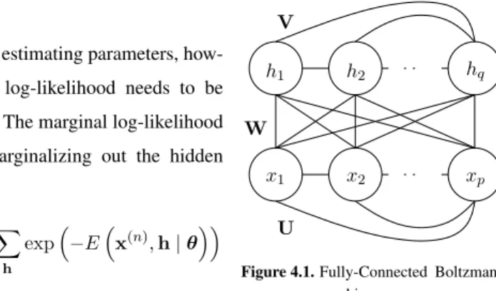
The chapter proceeds by describing a general Boltzmann machine of which all units, regardless of their types, are fully connected by undirected edges in Section 4.1. One important consequence of formulating the probability distribution of a Boltz-mann machine with a BoltzBoltz-mann distribution (see Section 2.3.2) is that an equiva-lent Boltzmann machine can always be constructed when the variables or units are transformed with, for instance, a bit-ﬂipping transformation. Based on this, in Sec-tion 4.1.1 theenhanced gradientwhich was proposed by the author in Publication I is introduced.

In Section 4.3, three basic estimation principles needed to train a Boltzmann ma-chine are introduced. They are Markov Chain Monte Carlo sampling, variational ap-proximation, and stochastic approximation procedure. An advanced sampling method, calledparallel tempering, whose use for training variants of Boltzmann machines was proposed in Publication III, Publication V and Publication VI for training vari-ants of Boltzmann machines, is described further in Section 4.3.1.

The remaining part of this chapter concentrates on more widely used variants of Boltzmann machines. In Section 4.4.1, an underlying mechanism based on the

(24)

con-ditional independence property of a Markov random ﬁeld is explained that justiﬁes re-stricting the structure of a Boltzmann machine. Based on this mechanism, a restricted Boltzmann machine and deep Boltzmann machine are explained in Section 4.4.2– 4.4.3.

After describing the restricted Boltzmann machine in Section 4.4.2, the author dis-cusses the connection between a product of experts and the restricted Boltzmann machine. This connection further leads to the learning principle of minimizing con-trastive divergence which is based on constructing a sequence of distributions using Gibbs sampling.

At the end of this chapter, in Section 4.5, the author discusses the connections be-tween the autoencoder and the Boltzmann machine found earlier by other researchers. The close equivalence between the restricted Boltzmann machine and the autoen-coder with a single hidden layer is described in Section 4.5.1. In due course, a Gaussian-Bernoulli restricted Boltzmann machine is discussed with itsmodiﬁed en-ergy functionproposed in Publication V. A deep belief network is subsequently discussed as a composite model of a restricted Boltzmann machine and a stochastic deep autoencoder in Section 4.5.2.

1.2.4 Unsupervised Neural Networks as the First Step

The last chapter before the conclusion deals with an important concept of pretraining, or initializing another potentially more complex neural network with unsupervised neural networks. This is ﬁrst motivated by the difﬁculty of training a deep multilayer perceptron in Section 3.4.1.

The ﬁrst section (Section 5.1) describes stacking multiple layers of unsupervised neural networks with a single hidden layer to initialize a multilayer perceptron, called layer-wise pretraining. This method is motivated in the framework of incrementally, or recursively, transforming the coordinates of input samples to obtain better repre-sentations. In this framework, several alternative building blocks are introduced in Sections 5.1.1–6.3.5.

In Section 5.2, we describe how the unsupervised neural networks such as Boltz-mann machines and deep belief networks can be used for discriminative tasks. A direct method of learning a joint distribution between an input and output is intro-duced in Section 5.2.1. A discriminative restricted Boltzmann machine and a deep belief network with the top pair of layers augmented with labels are described. A non-trivial method of initializing a multilayer perceptron with a deep Boltzmann ma-chine is further explained in Section 5.2.2.

The author wraps up the chapter by describing in detail how more complex gen-erative models, such as deep belief networks and deep Boltzmann machines, can be

(25)

initialized with simpler models such as restricted Boltzmann machines in Section 5.3. Another perspective based on maximizing variational lower bound is introduced to motivate pretraining a deep belief network by stacking multiple layers of restricted Boltzmann machines in Section 5.3.1–5.3.2. Section 5.3.3 explains two pretraining algorithms for deep Boltzmann machines. The second algorithm, called the two-stage pretraining algorithm, was proposed by the author in Publication VII.

1.2.5 Discussion

The author ﬁnishes the thesis by summarizing the current status of academic research and commercial applications of deep neural networks. Also, the overall content of this thesis is summarized. This is immediately followed by ﬁve subsections that discuss some topics that have not been discussed in, but are relevant to this thesis.

The ﬁeld of deep neural networks, or deep learning, is expanding rapidly, and it is impossible to discuss everything in this thesis. multilayer perceptrons, autoencoders and Boltzmann machines, which are the main topics of this thesis, are certainly not the only neural networks in the ﬁeld of deep neural networks. However, as the aim of this thesis is to provide a brief overview of and introduction to deep neural networks, the author intentionally omitted some models, even though they are highly related to the neural networks discussed in this thesis. One of those models is independent component analysis (ICA), and the author provides a list of references that present the relationship between the ICA and the deep neural networks in Section 6.3.1.

One well-founded theoretical property of most of deep neural networks discussed in this thesis is the universal approximator property, stating that a model with this property can approximate the target function, or distribution, with arbitrarily small error. In Section 6.3.2, the author provides the references to some earlier works that proved or described this property of various deep neural networks.

Compared to the feedforward neural networks such as autoencoders and multilayer perceptrons, it is difﬁcult to evaluate Boltzmann machines. Even when the struc-ture of the network is highly restricted, the existence of the intractable normalization constant requires using a sophisticated sampling-based estimation method to evalu-ate Boltzmann machines. In Section 6.3.3, the author points out some of the recent advances in evaluating Boltzmann machines.

The chapter ends by presenting recently proposed solutions to two practical mat-ters concerning training and building deep neural networks. First, a recently pro-posed method of hyper-parameter optimization is brieﬂy described, which relies on Bayesian optimization. Second, a standard approach to building a deep neural net-work that explicitly exploits the spatial structure of data is presented.

(26)

1.3 Author’s Contributions

This thesis contains ten publications that are closely related to and based on the basic principles of deep neural networks. This section lists for each publication the author’s contribution.

InPublication I,Publication II,Publication IIIandPublication IV, the author extensively studied learning algorithms for restricted Boltzmann machines (RBM) with binary units. By investigating potential difﬁculties of training RBMs, the au-thor together with the co-auau-thors of Publication I and Publication II designed a novel update direction called enhanced gradient, that utilizes the transformation invariance of Boltzmann machines (see Section 4.1.1). Furthermore, to alleviate selecting the right learning rate scheduling, the author proposed an adaptive learning rate algorithm based on maximizing the locally estimated likelihood that can adapt the learning rate on-the-ﬂy (see Section 6.3.3), in Publication II. In Publication III, parallel tempering which is an advanced Markov Chain Monte Carlo sampling algorithm, was applied to estimating the statistics of the model distribution of an RBM (see Section 4.3.1). Ad-ditionally, the author proposed and tested empirically novel regularization terms for RBMs that were motivated by the contractive regularization term recently proposed for autoencoders (see Section 3.3).

The author further applied these novel algorithms and approaches, including the enhanced gradient, the adaptive learning rate and parallel tempering to Gaussian-Bernoulli RBMs (GRBM) which employ Gaussian visible units in place of binary visible units inPublication V. In this work, those approaches as well as a modi-ﬁed form of the energy function (see Section 4.5.1) were empirically found to fa-cilitate estimating the parameters of a GRBM. These novel approaches were further applied to a more complex model, called a Gaussian-Bernoulli deep Boltzmann ma-chine (GDBM), inPublication VI.

InPublication VII, the author proposed a novel two-stage pretraining algorithm for deep Boltzmann machines (DBM) based on the fact that the encoder of a deep autoencoder performs approximate inference of the hidden units (see Section 5.3.3). A deep autoencoder trained during the ﬁrst stage is used as an approximate poste-rior distribution during the second stage to initialize the parameters of a DBM to maximize the variational lower bound of a marginal log-likelihood.

Unlike the previous work, the author moved his focus to a denoising autoencoder (see Section 3.3) trained with a sparsity regularization, inPublication VIII. In this work, mathematical motivation is given for sparsifying the states of hidden units when the autoencoder was trained with a sparsity regularization (see Section 3.2.5. The author proposes a simple sparsiﬁcation based on a shrinkage operator that was

(27)

empirically shown to be effective when an autoencoder is used to denoise a corrupted image patch with high noise.

InPublication XandPublication IX, two potential applications of deep neural networks were investigated. An RBM with Gaussian visible units was used to extract features from speech signal for speech recognition in highly noisy environment, in Publication X. This work showed that an existing system can easily beneﬁt from sim-ply adopting a deep neural network as an additional feature extractor. In Publication IX, the author applied a denoising autoencoder, a GRBM and a GDBM to a blind image denoising task.

(28)

2. Preliminary: Simple, Shallow Neural

Networks

In this chapter, we review several types of simple artiﬁcial neural networks that form the basis of deep neural networks1. By the termsimpleneural network, we refer to the neural networks that do not have any hidden units, in the case of supervised models, or have zero or one single layer of hidden units, in the case of unsupervised models.

Firstly, we look at a supervised model that consists of several visible, or input, units and a single output unit. There is a feedforward connection from each input unit to the output unit. Depending on the type of the output unit, this model can perform linear regression as well as a (binary) classiﬁcation.

Secondly, unsupervised models are described. We begin with a linear autoencoder that consists of several visible units and a single layer of hidden units, and show the connection with principal component analysis (PCA). Then, we move on to Hopﬁeld networks.

These models will be further discussed in a probabilistic framework. Each model will be re-formulated as a probabilistic model, and the correspondence between the parameter estimation from the perspectives of neural networks and probabilistic mod-els will be found. This probabilistic perspective will be useful later in interpreting a deep neural networks as a machine performing probabilistic inference and generation. At the end of this chapter, we discuss some conditions that distinguish deep neu-ral networks from the simple neuneu-ral networks introduced in the earlier part of this chapter.

1_{Note that we use the term}_{neural network}_{instead of}_artificial_{neural network. There should} not be any confusion, as this thesis specifically focuses only on artificial neural networks.

(29)

2.1 Supervised Model

Let us consider a case where a setDofNinput/output pairs is given:

D=

x(n), y(n)

N

n=1, (2.1)

wherex(n)∈Rpandy(n)∈Rfor alln= 1, . . . , N.

It is assumed that eachyis a noisy observation of a value generated by an unknown functionfwithx:

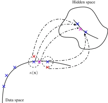
y=κ(f(x)). (2.2) whereκ(·)is a stochastic operator that randomly corrupts the input. Furthermore, it may be assumed thatx(n)is a noisy sample of an underlying distribution. Under this setting, a supervised model aims to estimatefusing the given training setD.

Often whenyis a continuous variable, the task is called aregressionproblem. On the other hand, whenyis a discrete variable corresponding to a class ofywith only a small number of possible outcomes, it is called aclassiﬁcationtask.

Now, we look at how simple neural networks can be used to solve these two tasks.

2.1.1 Linear Regression

A directed edge between two units or neurons indicates that the output of one unit ﬂows into the other one via the edge.2 _{It is possible to have multiple edges going}

out from a single unit and to have multiple edges coming in. Each edge has a weight value that ampliﬁes the signal carried by the edge.

A linear unitugathers allpincoming values ampliﬁed by the associated weights and outputs their sum:

u(x) =

p i=1

xiwi+b, (2.3)

wherewiis a weight of thei-th incoming edge, andbis a bias of the unit. With

this linear unit as an output unit, we can construct a simple neural network that can simulate the unknown functionf, given a training setD.

We can arrange the input and output units with the described linear units, as shown in Figure 2.1 (a). With a proper set of weights, this network then simulates the un-known functionfgiven an inputx.

The aim now becomes to ﬁnd a vector of weightsw = [w₁, . . . , wp]such that

the outputuof this neural network estimates the unknown functionfas closely as

2_{Although it is common to use the terms}_neuron_,_node_and_unit_{to indicate each variable in a} neural network, from here on, we use the termunit, only. An edge in a neural network is also commonly referred to as a synapse, synaptic connection or edge, but we use the termedge only in this thesis.

(30)

x1 x2 xp

y

(a) Linear Regression

x1 x2 xp

y

(b) Perceptron

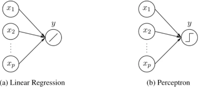
Figure 2.1.Illustrations of linear regression and perceptron networks. Note that the outputs of these two networks use different activation functions.

possible. If we assume Gaussian noise, this can be done by minimizing the squared error between the desired outputsy(n)_{and the simulated output}_u_(x(n)₎_with

respect tow: ˆ w= arg min w N n=1 y(n)−ux(n) 2 +λΩ (w, D), (2.4) whereΩandλare the regularization term and its strength. Regularization is a method for controlling the complexity of a model to prevent the model from overﬁtting to training samples.

If we assume the case of no regularization (λ= 0), we can ﬁnd the analytical solu-tion ofwˆby a simple linear least-squares method (see, e.g., Golub and van Van Loan, 1996). For instance,wˆ is obtained by multiplyingy= y(1), y(2), . . . , y(N) to a pseudo-inverse ofX= x(1),x(2), . . . ,x(N).

When there exists a regularization term, the problem in Eq. (2.4) may not have an analytical solution depending on the type of the regularization term. In this case, one must resort to using an iterative optimization algorithm (see, e.g., Fletcher, 1987). We iteratively compute updating directions to updatewsuch that eventuallywwill converge to a solutionwˆ that (locally) minimizes the cost function.

One exception is the ridge regression which regularizes the growth of theL₂-norm of the weight vectorwsuch that

Ω(w, D) =

p i=1

w2_i.

In this case, we still have an analytical solution

ˆ w= XX+λI −1 Xy.

It is, however, usual with other regularization terms that there is no analytical solu-tion. For instance, theleast absolute shrinkage and selection operator(lasso) (Tib-shirani, 1994) regularizes theL₁-norm of the weights, and the regularization term

Ω(w, D) =

p i=1

(31)

does not have an exact analytical solution.

Although we have considered the case of a one-dimensional outputy, this network can be extended to predict a multi-dimensional output. Simply, the network will require as many output units as the dimensionality of the outputy. The solution for the weightswcan be found in exactly the same way as before by solving the weights corresponding to each output simultaneously.

This simple linear neural network is highly restrictive in the sense that it can only approximate, or simulate, alinearfunction arbitrary well. When the unknown func-tionfis not linear, this network will most likely fail to simulate it. This is one of the motivations for considering a deep neural network instead.

2.1.2 Perceptron

The basic idea of the perceptron introduced by Rosenblatt (1958) is to insert a Heav-iside step functionφafter the summation in a linear unit, where

φ(x) = ⎧ ⎨ ⎩ 0, ifx <0 1, otherwise . (2.5)

The unituthen becomes nonlinear:

u(x) =φ p i=1 xiwi+b . (2.6)

This formula allows us to perform a binary classiﬁcation, where each sample is either classiﬁed asnegative(0) orpositive(1).

The illustration of a perceptron in Fig. 2.1 (b) shows that the perceptron is identical to the linear regression network except that the activation function of the output is a nonlinear step function.

Consider a case where we have again a training setDof input/output pairs. How-ever, now each outputy(n)is either0or1. Furthermore, eachy(n)was generated fromx(n)by an unknown functionf, as in Eq. (2.2). As before, we want to ﬁnd a set of weightswsuch that the perceptron can approximate the unknown functionf

as closely as possible.

In this case, this is considered aclassificationtask rather than aregressionas there is a finite number of possible values fory. The task of the perceptron is to figure out to which class each samplexbelongs.

A perceptron can perfectly simulate the unknown functionf, when the training samples arelinearlyseparable (Minsky and Papert, 1969). Linear separability means that there exists a linear hyperplane that separatesx(n)that belongs to the positive class from those that belong to the negative class (see Fig. 2.2). With a correct set of

(32)

(a) Linearly separable (b) Nonlinearly separable Figure 2.2.(a) Samples are linearly separable. (b) They are separable, but not linearly.

weightsw∗, the linearseparating hyperplanecan be characterized by

p i=1

xiw∗i+b∗= 0

The perceptron learning algorithm was proposed to estimate the set of weights The algorithm iteratively updates the weightswoverNtraining samples by the following rule:

w←w+ηy(n)−ux(n)

x(n).

This will converge to the correct solution as long as the given training set is linearly separable.

Note that it is possible to use any other nonlinear saturating function whose range is limited from above and below so that it can approximate the Heaviside function. One such example is a sigmoid function whose range is[0,1]:

φ(x) = 1

1 + exp (−x). (2.7)

In this case, a given samplexis classiﬁed positive if the output is greater than, or equal to,0.5, and otherwise as negative. Another possible choice is a hyperbolic tangent function whose range is[−1,1]:

φ(x) = tanh(x). (2.8)

The set of weights can be estimated in another way by minimizing the difference between the desired output and the output of the network, just like in the simple linear neural network. However, in this case the cross-entropy cost function (see, e.g. Bishop, 2006) can be used instead of the mean squared error:

ˆ w= arg min w N n=1 −y(n)logu x(n) −1−y(n) log 1−u x(n) +λΩ (w, D). (2.9)

(33)

Unlike the simple linear neural network, this does not have an analytical solution, and one needs to use an iterative optimization algorithm.

As was the case with the simple linear neural network, the capability of the per-ceptron is limited. It only works well when the classes arelinearlyseparable (see, e.g., Minsky and Papert, 1969). For instance, a perceptron cannot learn to compute an exclusive-or (XOR) function. In this case, any non-noisy samples from the XOR function are not separable with a linear boundary.

It has been known that a network of perceptrons, having between the input units and the output unit one or more layers of nonlinear hidden units that do not correspond to either inputs or outputs, can solve classiﬁcation tasks where classes are not linear separable, such as the XOR function (see, e.g., Touretzky and Pomerleau, 1989). This makes us consider adeepneural network also in the context of classiﬁcation.

2.2 Unsupervised Model

Unlike in supervised learning, unsupervised learning considers a case where there is no target value. In this case, the training setDconsists of only input vectors:

D=x(n)

N

n=1. (2.10)

Similarly to the supervised case, we may assume that eachxinDis a noisy obser-vation of an unknown hidden variable such that

x=f(h). (2.11) Whereas we aimed to ﬁnd the function or mappingf given both input and output previously in supervised models, our aim here is to ﬁnd both the unknown function

fand the hidden variablesh∈Rq. This leads tolatent variable modelsin statistics (see, e.g., Murphy, 2012).

This is, however, not the only way to formulate an unsupervised model. Another way is to build a model that learns direct relationships among the input components

x₁, . . . , xp. This does not require any hidden variable, but still learns an (unknown)

structure of the model.

2.2.1 Linear Autoencoder and Principal Component Analysis

In this section, we look at the case where hidden variables are assumed to have lin-early generated training samples. In this case, it is desirable for us to learn not only an unknown functionf, but also another functiongthat is an (approximate) inverse function off. Opposite tof,grecognizes a given sample by ﬁnding a corresponding

(34)

x1 x2 xp ˜ x1 ˜ x2 ˜ xp h1 hq

(a) Linear Autoencoder

x1 x2 x3 xp

(b) Hopﬁeld Network

Figure 2.3.Illustrations of a linear autoencoder and Hopfield network. An undirected edge in the Hop-field network indicates that signal flows in both ways.

state of the hidden variables.3

Let us construct a neural network with linear units. There are as many input units aspcorresponding to components of an input vector, denoted byx, andqlinear units that correspond to the hidden variables, denoted byh. Additionally, we add another set ofplinear units, denoted byx˜. We connect directed edges fromxtohand from

htox˜. Each edgeeijwhich connects thei-th input unit to thej-th hidden unit has a

corresponding weightwij. Also, edgeejkwhich connects thej-th hidden unit to the k-th output unit has its weightujk. See Fig. 2.3 (a) for the illustration.

This model is called a linear autoencoder.4_{The encoder of the autoencoder is}

h=f(x) =Wx+b, (2.12)

and the decoder is

˜

x=g(h) =Uh(x) +c, (2.13)

where we uses the matrix-vector notation for simplicity. W = [wij]_p_×_q are the

encoder weights, U = [ujk]_q_×_p the decoder weights, andbandcare the hidden

biases and the visible biases, respectively. It is usual to call the layer of the hidden units abottleneck.5_{Note that without loss of generality we will omit biases whenever}

it is necessary to make equations uncluttered.

In this linear autoencoder, the encoder in Eq. (2.12) acts as an inverse function

gthat recognizes a given sample, whereas the decoder in Eq. (2.13) simulates the unknown functionfin Eq. (2.11).

If we tied the weights of the encoder and decoder so thatW =U, we can see the connection between the linear autoencoder and the principal component analysis

3_{Note that it is not necessary for}_g_{to be an explicit function. In some models such as sparse} coding in Section 3.2.5,gmay be deﬁned implicitly.

4_{The same type of neural networks is also called}_{autoassociative}_{neural networks. In this} thesis, however, we use the termautoencoderwhich has become more widely used recently. 5_{Although the term}_bottleneck_{implicitly implies that the size of the layer is smaller than that} of either the input or output layers, it is not necessarily so.

(35)

(PCA). Although there are many ways to formulate PCA (see, e.g. Bishop, 2006), one way is to use a minimum-error formulation6that minimizes

J(θ) =1 2 N n=1 x(n)−x˜(n)2 2. (2.14)

The minimum of Eq. (2.14) is in fact exactly the solution the linear autoencoder aims to ﬁnd.

This connection and equivalence between the linear autoencoder and the PCA have been noticed and shown by previous research (see, for instance, Oja, 1982; Baldi and Hornik, 1989). However, it should be reminded that minimizing the cost function in Eq. (2.14) by an optimization algorithm is unlikely to recover the principal compo-nents, but an arbitrary basis of the subspace spanned by the principal compocompo-nents, unless we explicitly constrain the weight matrix to be orthogonal.

This linear autoencoder has several restrictions. The most obvious one is that it is only able to learn a correct model when the unknown functionfis linear. Secondly, due to its linear nature, it is not possible to model any hierarchical generative process. Adding more hidden layers is equivalent to simply multiplying the weight matrices of additional layers, and this does not help in any way.

Another restriction is that the number of hidden unitsqis upper-bounded by the input dimensionalityp. Although it is possible to useq > p, it will not make any difference, as it does not make any sense to use more thanpprincipal components in PCA. This could be worked around by using regularization as in, for instance, sparse coding (Olshausen and Field, 1996) or independent component analysis (ICA) with reconstruction cost (Le et al., 2011b).

As was the case with the supervised models, this encourages us to investigate more complex, overcomplete models that have multiple layers of nonlinear hidden units.

2.2.2 Hopﬁeld Networks

Now let us consider a neural network consisting of visible units only, and each visible unit is anonlinear,deterministicunit, following Eq. (2.6), that corresponds to each component of an input vectorx. We connect each pair of the binary unitsxiandxj

with an undirected edgeeijthat has the weightwij, as in Fig. 2.3 (b). We add to each

unitxia bias termbi. Furthermore, let us deﬁne anenergyof the constructed neural

network as −E(x|θ) =1 2 i=j wijxixj+ i xibi, (2.15)

6_{Actually the minimum-error formulation minimizes the mean-squared error}_E _x₋_˜_x2 2

which is in most cases not available for evaluation. The cost function in Eq. (2.14) is an approximation to the mean-squared error using a ﬁnite number of training samples.

(36)

whereθ= (W,b). We call this neural network a Hopfield network (Hopfield, 1982). The Hopfield network aims to finding a set of weights that makes the energy of the presented patterns low via the training setD=x(1), . . . ,x(N)(see, e.g., Mackay, 2002). Given a fixed set of weights and an unseen, possibly corrupted input, the Hopfield network can be used to find a clean pattern by finding the nearestmodein the energy landscape.

In other words, the weights of the Hopﬁeld network can be obtained by minimizing the following cost function given a setDof training samples:

J(θ) = N n=1 E x(n)θ . (2.16)

The learning rule for each weightwijcan be derived by taking a partial derivative

of the cost functionJwith respect to it. The learning rule is

wij←wij− η N N n=1 ∂Ex(n)|θ ∂wij =wij+ η N N n=1 x(_in)x(_jn)=wij+ηxixj_d, (2.17)

whereηis a learning rate andx_Prefers to the expectation ofxover the distribution

P. We denote by d the data distribution from which samples in the training setD

come. Similarly, a biasbican be updated by

bi=bi+ηxid. (2.18)

This learning rule is known as the Hebbian learning rule (Hebb, 1949). This rule states that the weight between two units, or neurons, increases if they are active to-gether. After learning, the weight will be strongly positive, if the activities of the two connected units are highly correlated.

With the learned set of weights, we can simulate the network by updating each unit

xiwith xi=φ ⎛ ⎝ j=i wijxj+bi ⎞ ⎠, (2.19)

whereφis a Heaviside function as in Eq. (2.6).

It should be noticed that because the energy function in Eq. (2.15) is not lower bounded and the gradient in Eq. (2.17) does not depend on the parameters, we may simply set each weight by

wij=cxixj_d,

wherecis an arbitrary , positive constant, given a ﬁxed set of training samples. An arbitrarycis possible, since the output of (2.19) is invariant to the scaling of the parameters.

(37)

In summary, the Hopﬁeld network memorizes the training samples and is able to retrieve them, starting from either a corrupted input or a random sample. This is one way of learning an internal structure of a given training set in an unsupervised manner.

The Hopfield network learns the unknown structure of training samples. However, it is limited in the sense that only direct correlations among visible units are modeled. In other words, the network can only learn second-order statistics. Furthermore, the use of the Hopfield network is highly limited by a few fundamental deficiencies in-cluding the emergence of spurious states (for more details, see Haykin, 2009). These encourage us to extend the model by introducing multiple hidden units as well as making them stochastic.

2.3 Probabilistic Perspectives

All neural network models we have described in this chapter can be re-interpreted from a probabilistic perspective. This interpretation helps understanding how neural networks performgenerativemodeling andrecognizepatterns in a novel sample. In this section, we brieﬂy explain the basic ideas involving probabilistic approaches to machine learning problems and their relationship to neural networks.

For more details on probabilistic approaches, we refer the readers to, for instance, (Murphy, 2012; Barber, 2012; Bishop, 2006).

2.3.1 Supervised Model

Here we consider discriminative modeling from the probabilistic perspective. Again, we assume that a setDofN input/output pairs, as in Eq. (2.1), is given. The same model in Eq. (2.2) is used to describe how the setDwas generated. In this case, we can directly plug in a probabilistic interpretation.

Let each componentxiofxbe a random variable, but for now ﬁxed to a given

value. Also, we assume that the observation ofyis corrupted by additive noise

which is another random variable. Then, the aim of discriminative modeling in a probabilistic approach is to estimate or approximate the conditional distribution of yet another random variableygiven the inputxand the noiseparameterized7byθ, that is,p(y|x,θ).

The prediction of the outputyˆgiven a new samplexcan be computed from the

7_{It is possible to use non-parametric approaches, such as Gaussian Process (GP) (see, e.g.,} Rasmussen and Williams, 2006), which do not have in principle any explicit parameter. How-ever, we may safely use the parametersθby including the hyper-parameters of, for instance, kernel functions and potentially even (some of) the training samples.

(38)

conditional distributionp(y|x,θ˜)with the estimated parametersθ˜. It is typical to use the mean of the distribution as a prediction and its variance as a conﬁdence.

Linear Regression

A probabilistic model equivalent to the previously described linear regression net-work can be built by assuming that the noisefollows a Gaussian distribution with zero mean and its variance is ﬁxed tos2. Then, the conditional distribution ofygiven a ﬁxed inputxbecomes

p(y|x, s2) =N y p i=1 xiwi+b, s2 ,

whereNym, s2is a probability density of the scalar variableyfollowing a Gaus-sian distribution with the meanmand variances2. A linear relationship between the input and output variables has been assumed in computing the mean of the distribu-tion.

The parameterswiandbcan be found by maximizing the log-likelihood function

L(w, b) =− N n=1 y(n)₋p i=1x(n)i wi−b 2 2s2 +C, (2.20)

where the constant C does not depend on any parameter. This way of estimatingwˆi

andˆbto maximizeLis called maximum-likelihood estimation (MLE). If we assume a ﬁxed constants2, maximizingLis equivalent to minimizing

N n=1 y(n)−u(x(n)) 2

using the deﬁnition of the output of a linear unitu(x)from Eq. (2.3). This is identical to the cost function of the linear regression network given in Eq. (2.4) without a regularization term.

A regularization term can be inserted by considering the parameters as random variables. When each weight parameterwi is given a prior distribution, the

log-posterior distributionlogp(w | x, y)of the weights can be written, using Bayes’ rule8_{, as}

logp(w|x, y) = logp(y|x,w) + logp(w) +const., 8_{Bayes’ rule states that}

p(X|Y) =p(Y |X)p(X)

p(Y) , (2.21)

where bothXandYare random variables. One interpretation of this rule is that the posterior probability ofX given Y is proportional to the product of the likelihood (or conditional probability) ofY givenXand the prior probability ofX. If both the conditional and prior distributions are speciﬁed, the posterior probability can be evaluated as their product, up to the normalization constant or evidencep(Y).

(39)

x1 x2 xp y x(n) h(n) σ2 N W

(a) Naive Bayes (b) Probabilistic PCA

Figure 2.4.Illustrations of the naive Bayes classifier and probabilistic principal component analysis. The naive Bayes classifier in (a) describes the conditional independence of each component of input given its label. In both figures, the random variables are denoted with circles (a gray circle indicates anobservedvariables), and other parameters are without surrounding circles. The plate indicates that there areNcopies of a pair ofx(n)andh(n). For details on probabilistic graphical models, see, for instance, (Bishop, 2006).

where the constant term does not depend on the weights. If, for instance, the prior distribution of each weightwiis a zero-mean Gaussian distribution with its variance

ﬁxed to₂1_λ, the log-posterior distribution given a training setDbecomes

logp w (x(n), y(n))N n=1 =L(w, b)−λ p i=1 w2_i.

Maximizing this posterior is equivalent to ridge regression (Hoerl and Kennard, 1970). When the log-posterior is maximized instead of the log-likelihood, we call it a maximum-a-posteriori estimation (MAP), or in some cases, penalized maximum-likelihood es-timation (PMLE).

Logistic Regression: Perceptron

As was the case in our discussion on perceptrons in Section 2.1.2, we consider a binary classiﬁcation task.

Instead of Eq. (2.2) where it was assumed that the outputywas generated from an inputxthrough an unknown functionf, we can think of a probabilistic model where the samplexwas generated according to the conditional distribution given its label9 y, whereywas chosen according to the prior distribution. In this case, we assume that we know the forms of the conditional and prior distributionsa priori. See Fig. 2.4 (a) for the illustration of this model, which is often referred to as the naive Bayes model (see, e.g., Bishop, 2006).

Based on this model, the aim is to ﬁnd a class, or a label, that has the highest posterior probability given a sample. In other words, a given sample belongs to a class 1, if

p(y= 1|x)≥1 2,

9_A_label_{of a sample tells to which}_class_{the sample belongs. Often these two terms are}