Outlier Detection and Multicollinearity in Sequential Variable Selection: A Least Angle Regression-Based Approach

OUTLIER DETECTION AND

MULTICOLLINEARITY IN SEQUENTIAL

VARIABLE SELECTION:

A LEAST ANGLE REGRESSION-BASED

APPROACH

A Dissertation

Presented to the Faculty of the Graduate School of Cornell University

in Partial Fulfillment of the Requirements for the Degree of Doctor of Philosophy

by

Kelly Meredith Kirtland January 2017

c

2017 Kelly M. Kirtland ALL RIGHTS RESERVED

OUTLIER DETECTION AND MULTICOLLINEARITY IN SEQUENTIAL VARIABLE SELECTION:

A LEAST ANGLE REGRESSION-BASED APPROACH Kelly Meredith Kirtland, Ph.D.

Cornell University 2017

As lasso regression has grown exceedingly popular as a tool for coping with variable selection in high-dimensional data, diagnostic methods have not kept pace. The primary difficulty of outlier detection in high-dimensional data is the inability to examine all subspaces, either simultaneously or sequentially. I ex-plore the impact of outliers on lasso variable selection and penalty parameter estimation, and propose a tree-like outlier nominator based on the LARS algo-rithm. The least angle regression outlier nomination (LARON) algorithm fol-lows variable selection paths and prediction summaries for the original data set and data subsets after removing potential outliers. This provides visual insight into the effect of specific points on lasso fits while allowing for a data-directed exploration of various subspaces.

Simulation studies indicate that LARON is generally more powerful at de-tecting outliers than standard diagnostics applied to Lasso models after fitting a model. One reason for this improvement is that observations with unusually high influence can inflate the penalty parameter and result in a severely under-fit model. We explore this result through simulations and theoretically using a Lasso homotopy adapted for online observations. Additionally, LARON is able to explore multiple subspaces while post-hoc diagnostics rely on a variable se-lection that has already occurred under possible influence of an unusual

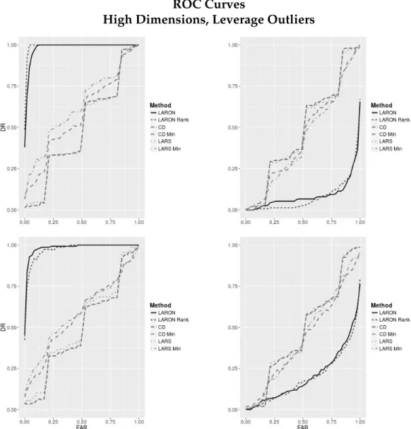
obser-vation. However, LARON underperforms random nomination when attempt-ing to detect high leverage, non-influential points located in minor eigenvalue directions in high dimensional settings. The lack of detection appears to result from a robustness in Lasso’s variable selection process against such points.

A new R package implementing the LARON algorithm is presented and its functionality to detect multicollinearity in the data, even when masked by high leverage points, described. This package is then used to analyze data created by simulation and several real data sets.

BIOGRAPHICAL SKETCH

Academia has surrounded Kelly Kirtland ever since she was a little girl grow-ing up near Hamilton College in Clinton, NY. Although she had intended to dedicate her life to a career in music, she developed a love for math during her time at Wheaton College in Illinois. Kelly was introduced to statistics and com-puter programming in the summer before her senior year when she attended the Summer Institute for Training in Biostatistics sponsored by North Carolina State University and the Duke Clinical Research Institute. Despite an unbear-ably hot southern summer, the staunch northerner found statistics so interesting that she decided to pursue a graduate degree in the field. She was accepted into the M.S./Ph.D. program at Cornell University and began her studies immedi-ately after completing her B.S. in Mathematics.

At Cornell she met her husband Joe who, despite being a physicist, managed to sweep her off her feet through his patience and good humor. After their first year of marriage, Joe received a job at Alfred University, causing the Kirtlands moved two hours away from Ithaca just as Kelly was beginning a new research project under Dr. Paul Velleman. After a year working exclusively on her the-sis, Kelly was offered an adjunct position at Alfred University while attending a local game night; a year later, she applied for and was awarded a visiting profes-sor position in the Division of Mathematics and Computer Science, which she has maintained and will continue to hold after the completion of her degree.

With the completion of her Ph.D. in January of 2017, Kelly fully intends to dive back into the hobbies she loves and has missed sorely during the many years since she began her degree: singing and playing the piano, los-ing to her husband at tennis, hiklos-ing in the Adirondacks, playlos-ing board games with friends, embroidery, traveling, staying involved in her Orthodox Christian

ACKNOWLEDGEMENTS

I would never have been able to complete this degree without the help and support of many of the Cornell University faculty and staff. Marty Wells was foundational in seeing the form of this thesis somewhere in my scattered ideas. Jacob Bien provided essential insight into the Lasso, recommending papers and discussing ideas. Giles Hooker, Bea Johnson, and Diana Drake and Bea Johnson helped me to navigate the sea of inexplicable forms and allowing me to workin

absentia.

Thank you to my advisor Paul Velleman, who made all of this possible. Paul gave me a chance to continue my degree when few others would have under-taken the task. He was a constant fount of optimism and much needed perspec-tive. He and his wife Sue opened to me their hearts and their home, always taking an interest in me as a person beyond my work.

My family and friend’s unswerving support has been amazing during the many, many years I have remained in school. Mom and Dad, thank you for your love and encouragement, for never losing faith in me, and being proud of me no matter what. Thank you to the rest of my wonderful family, St. John the Baptist Orthodox Church, and the many, many dear friends too numerous to name who have fed me, called me, prayed for me, and given me a reason to get away from the computer and out of the house at least three times each year.

And finally, thank you to my husband Joe who continues to be the best thing to have come out of my graduate school experience. I could never have made it through without your constant support, empathy, love, and patience. You have always been there as a voice of encouragement, reason, and faith, my best friend and better half. I love you with every particle of my being!

TABLE OF CONTENTS

Biographical Sketch . . . iii

Dedication . . . v

Acknowledgements . . . vi

Table of Contents . . . vii

List of Tables . . . ix List of Figures . . . x 1 Introduction 1 1.1 Overview . . . 1 1.1.1 Curse of Dimensionality . . . 4 1.2 Outliers . . . 5 1.2.1 Characteristics . . . 6

1.2.2 Diagnostic Measures and Procedures . . . 8

1.3 Multicollinearity . . . 13

1.4 Lasso Model . . . 14

1.4.1 Bayes Perspective . . . 16

1.4.2 Properties and Optimality Conditions . . . 17

1.4.3 Penalty Parameter Forms . . . 20

2 Lasso Estimation 22 2.1 Overview of Estimation Methods . . . 22

2.2 Selection of Penalty Parameters . . . 23

2.2.1 Outliers and the Penalty Parameter . . . 26

2.2.2 Multicollinearity and the Penalty Parameter . . . 30

2.3 Least Angle Regression . . . 31

2.3.1 Geometric Motivation . . . 32

2.3.2 Algorithm Details . . . 33

2.4 Homotopy for Sequential Observations . . . 35

3 Least Angle Regression Outlier Nomination 42 3.1 Algorithm . . . 42

3.1.1 Why use LARS? . . . 43

3.1.2 Theoretical Example . . . 46 3.2 Simulation Studies . . . 48 3.2.1 Simulation Set-up . . . 48 3.2.2 Outlier Detection . . . 51 3.3 Examples . . . 60 3.3.1 Simulated Example . . . 60 3.3.2 Diabetes Data . . . 63 3.3.3 Riboflavin Data . . . 65

4 Laron Package in R 77

4.1 Main function . . . 77

4.1.1 Influence Measures and Cutoffs for Branching Process . . 80

4.1.2 Other Branching Options . . . 83

4.1.3 Reading Branch Path Plots . . . 84

4.2 Outlier Nomination . . . 86

4.2.1 Nomination Criteria . . . 87

4.2.2 Reading Outlier Plots . . . 90

4.3 Collinearity . . . 91

4.3.1 Interpreting Collinear Graphs . . . 93

4.4 Branch Information . . . 95

5 Conclusion 97 5.1 Summary of findings . . . 97

5.2 Future work . . . 98

A Complete options for functions in laron package 103 A.0.1 laron_{function . . . 103}

A.0.2 outliersfunction . . . 104

A.0.3 collinearityfunction . . . 105

A.0.4 plot_{function for}laron_,outlier_{, and}multicol_{objects 106} A.0.5 SRGridplotting function . . . 108

A.0.6 summaryandprintfunctions forlaronobjects . . . 109

A.0.7 summary_andprint_{functions for}outlier_{objects . . . 109}

A.0.8 summaryandprintfunctions formulticolobjects . . . 110

A.0.9 summaryandprintfunctions forbranchobjects . . . . 111 B Additional Information on Simulation Results and the Riboflavin

Data 113

LIST OF TABLES

3.1 Description of variables in the diabetes dataset. . . 62

3.2 VIFs and pairwise correlations among the diabetes predictors . . 64

3.3 Outlier nomination under various nomination criteria . . . 68

3.4 Correlated predictor groups in the riboflavin data . . . 71

3.5 AIC values for models fit to the riboflavin data. . . 72

3.6 Coefficient values for models fit to the riboflavin data with cor-related groups . . . 75

B.1 High Residual Outliers: False Alarms . . . 114

B.2 High Residual Outliers: Detection Rates . . . 114

B.3 High Residual Outliers: Outlier Info . . . 115

B.4 Leverage Outliers: False Alarms . . . 116

B.5 Leverage Outliers: Detection Rates . . . 117

B.6 Leverage Outliers: Outlier Info . . . 118

B.7 Full table of coefficient values for riboflavin model fits. . . 119

LIST OF FIGURES

2.1 Cross-validation plots for penalty parameter selection, with and without outliers . . . 27 2.2 Change in active set size and prediction error of CV-selected

Lasso models in the presence of outliers. . . 29 2.3 Change in active set size and prediction error of CV-selected

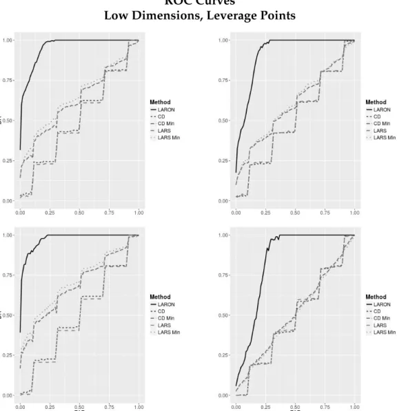
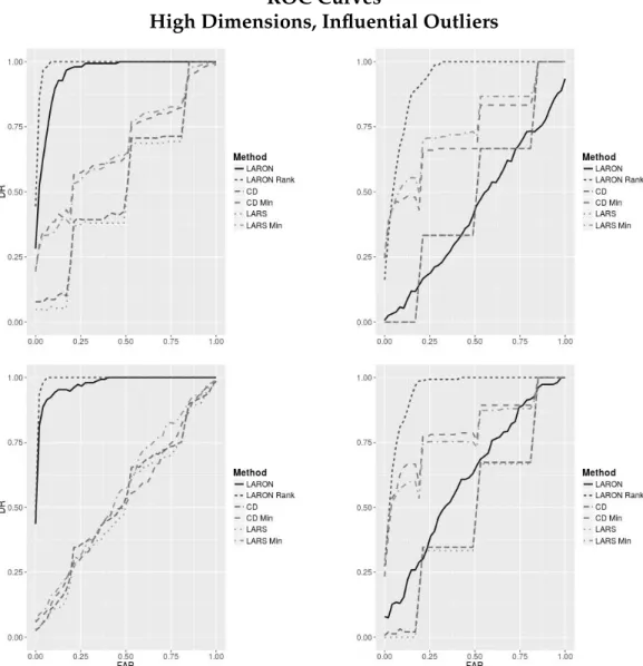
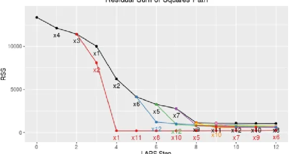
Lasso model in the presence of autoregressive multicollinearity. . 30 3.1 Multicollinearity masked by outliers. . . 45 3.2 Confusion matrix . . . 52 3.3 ROC curves for low-dimensional, influential outlier detection . . 54 3.4 ROC curves for low-dimensional, high leverage point detection . 55 3.5 ROC curves for high-dimensional, influential outlier detection . 57 3.6 ROC curves for high-dimensional, high leverage point detection 58 3.7 LARON RSS path for simulated data set . . . 61 3.8 Outlier nomination RSS for diabetes dataset with log-transformed

response. . . 63 3.9 Selection ratio versus average Cook’s distance from the LARON

analysis of the riboflavin data . . . 65 3.10 Fitted v. true response values for prior model fits to the

ri-boflavin data. . . 66 3.11 Fitted v. true response values of models selected for the

ri-boflavin data with CV-selected penalty parameters, with and without outliers. . . 67 3.12 10-fold cross-validation for riboflavin data with and without

out-liers . . . 70 3.13 Riboflavin production v. YEZB at predictor, the univariate

direc-tion wherein the leverage of case 61 may most clearly be seen. . . 72 3.14 Correlation heat map for selected variables in riboflavin data set. 76 4.1 Thelaronpackage’s diagnostic plots for thesim1data set. . . . 81 4.2 Collinearity plots for thediabetes_{data. . . . 94} 5.1 Run times forlaronpackage . . . 100

CHAPTER 1 INTRODUCTION

1.1

Overview

High dimensional data (commonly referred to as “pgreater thann”) introduce many unique challenges to the data analyst. All analyses focus on at least one of the following interrelated goals: variable selection, model interpretation, and prediction. It is necessary to assume that any relevant information exists only in a low-dimensional subspace, and discovery of this subspace, i.e. variable se-lection, should be of primary importance. Only once this has been completed is it possible to perform model estimation for the purposes of interpretation. It does not make sense to interpret coefficient values if the important variables are omitted from the subspace or their effects are swamped by unimportant vari-ables. Optimal internal prediction may be achieved with alternative subspaces, but external prediction may suffer without correct variable selection. For ex-ample, the “noise accumulation” from including too many extraneous variables or utilizing a subspace of a higher dimension than is optimal tends to decrease prediction accuracy (see [21] and [23]).

The impact of outlying data points is frequently acknowledged in standard regression fits. Due to model-fitting tendencies to reduce prediction error, some points may pull the model towards themselves, decreasing the residual at that point and making the data point appear ordinary; this self-justifying behavior can make it quite difficult to detect an outlier numerically, which is frequently the only option in multivariate regression. There are two broad categories of outlier detection methodologies: they may be called “direct” and “indirect”, as

in [30], or “diagnosis” and “accommodation” in [35]. Direct methods are largely concerned with performing diagnostics that measure the change to a model or estimator conditioned on the removal of a subset of observations. Indirect meth-ods prefer to utilize models that are robust against unusual observations (i.e. models that are difficult for a small set of points to “bend”), and use the results of these models as the yardstick for unusual behavior.

Models intended for variable selection, particularly those in the high-dimensional case, provide little in the way of robustness against outlying obser-vations. Indeed, due to the vast emptiness of the data space, there is a sense in whichevery observation is unusual. Subset selection, for example, was specif-ically cited by Tibshirani in [62] as susceptible to changes in model selection and prediction accuracy due to “small changes in the data”. Ridge regression, while in a sense robust against influential observations (by down-weighting points unusual in low-eigenvalue directions; see [46]), does not provide sparse variable selection. The LAD-Lasso method proposed by Wang, Li, and Jiang [67] is only robust against heavy-tailed residuals rather than influential points. Therefore a direct approach appears to be more suitable than indirect meth-ods. Unfortunately, known diagnostic measures can only be calculated on a low-dimensional subspace. As it is generally impossible to perform exhaustive subspace searches, this subspace is generally selected using a non-robust model fit to a potentially contaminated data set. Therefore a common mode of model diagnostic in this context involves utilizing an indirect approach (i.e. build a model using all observations, then compare observations to the model) with a model that is not sufficiently stable for the purpose.

in multiple regression scenarios with sparse coefficient vectors. It is widely used in datasets from the fields of genetics and compressive sensing, among others. There have been suggestions for adaptations of the Lasso in order to simulta-neously perform outlier detection, however these require either unreasonable conditions (such as knowing a priori that a significant subset of the the obser-vations are not outliers, as in [64]) or estimation of an additional penalty pa-rameter. The first is clearly not suitable in common model fitting problems, and the second is likely an issue since outliers can influence data-driven estimates of penalty parameters, discussed further in Section 2.2.1.

Instead, I have examined the computation methods for determining a Lasso fit. Estimating a lasso fit relies on algorithms that sequentially or iteratively update the coefficient estimates and the set of variables active in the model. Influential observations can influence a single step in the process and the algo-rithm may never be able to recover. This error may even be compounded in subsequent iterations. Therefore it is important to examine the impact of obser-vations during each step in the process.

The algorithm proposed here attempts to do just that. It incorporates stan-dard lower-dimensional diagnostic measures into every step of the LARS algo-rithm for computing the Lasso. LARS, as with other Lasso algoalgo-rithms, produces a sequence of possible models indexed on the amount of penalization applied to the coefficients. Thus I propose building alternative paths whenever an ob-servation or set of obob-servations would lead to utilizing an alternative subspace in the model. Implementing sequential diagnostics in this manner provides the following benefits:

process.

2. Allowing the subspace on which diagnostics will be performed to vary dynamically.

3. Observing the improvement in prediction accuracy through the removal of certain observations.

1.1.1

Curse of Dimensionality

Keough and Mueen [39] provide an excellent overview of the “curse of dimen-sionality”. The phrase has been used to connote different things, but one im-portant interpretation of this idea is the decentralization of space as the number of dimensions increases, as exemplified by taking the ratio of the volumes of the unit sphere and the unit square. As the number of dimensions goes up, the unit sphere contains an insignificant amount of volume relative to the unit square (i.e. the majority of space moves further and further from the center). In standard modeling procedures it also may be used to refer to the exponentially larger number of cases required to achieve equivalent accuracy.

A major implication of this in the context of outlier detection in high-dimensional data is in the form of measurement. Distance does not generalize intuitively into higher dimensions; there is a sense in which all points in space are considered equally far apart. This can be a problem when it comes to outlier detection since it is common to define outliers as points which are “far” (ac-cording to some metric) from the main body of data. With high dimensional data, however, it doesn’t particularly make sense to utilize this idea of distance. Another approach is to incorporate some idea of “influence” on an estimator

instead. This is not necessarily better, as all observations exert a great deal of in-fluence over models. The removal of a single point from any high-dimensional data set (however clean) may result in chaotic behavior in subset selection; the Lasso, elastic net, and ridge regression are considered more stable.

1.2

Outliers

There are several inherent challenges with outlier detection in general. Visual detection, the most effective method, is rarely possible for p > 3. Outliers tend to be self-justifying because they generate parameter estimates that conform to the anomalous values, so the examination of recalculated statistics after the re-moval of these points is usually necessary before their influence can be detected. Outlying points may also exist in groups called microclusters [53], requiring that the entire microcluster be removed before the influence of any individual point can be identified.

The detection of outliers is an essential step toward reaching the ultimate goal of every analyst: better understanding of the data and its implications for the population of interest. The bending of a model fit to a disproportion-ately small number of observations can result in poor predictive capabilities for new observations and incorrect interpretations of coefficient estimates. Lo-cating unusual observations in multivariate space may also be an end in itself, such as in determining credit card fraud. This type of analysis may also be called “anomaly” detection. Outlier detection allows analysts to correct or omit values that are known to be incorrect prior to use in estimation or inferential procedures, identify cases which do not belong to the population of interest, or

discover a previously unforeseen subgroup of the population which may open new and interesting areas of research.

The causes of outliers in data are so diverse that there is no way to prescribe a general solution to their existence. If any outliers are noticed, the analyst must carefully explore the specific nature of the extraordinary point, fix any identi-fiable errors, and consider the modeling goals before determining a course of action. One should not be hasty and automatically remove any observation that seems to counteract a perceived trend. It is also important to recognize that there are certainly scenarios which warrant such removal. It is more common to hear invectives against the former, though the latter may cause similar prob-lems. I have personally heard an illustrative story from a biologist who was studying the movements of fish. During the experiment, one of the electronic sensors attached to a fish malfunctioned and caused the fish to have a seizure. This one observation altered his conclusions, but he was not allowed to remove it for publishing.

1.2.1

Characteristics

The term “outliers” is one for which there is not a single agreed-upon definition. In the vernacular and in common statistical practice, it is generally intended to convey the idea presented by Grubbs [29]: “An outlying observation, or out-lier, is one that appears to deviate markedly from other members of the sample in which it occurs.” Another similar definition was proposed somewhat more recently by Bendle, Barnett & Lewis [6]: “An observation (or subset of observa-tions) which appears to be inconsistent with the remainder of that set of data.”

However, an interpretation of the term in the context of linear models was pre-sented by Chatterjee and Hadi [12]: “an observation for which the studentized residual is large in magnitude compared to other observations in the data set.”; that is, an observation which does not follow the general model fit to the data set. I will use the term outlier in the sense of its more general definition, and discuss Chatterjee and Hadi’s interpretation simply as a particularcharacteristic that may be exhibited by an outlier.

There are two main qualities which may be exhibited by an outlier:

1. High Leverage. Observations with high leverage are unusual in the

pre-dictor space and are defined identically to multivariate space ouliers as above. Regression estimates are highly susceptible to changes in the re-sponse value of these points.

2. Large Residual. In this context, the large residual refers to an extraordinary

deviation from the “true” model, i.e. the model which best fits the majority of observations. (In practice, this point may not have an unusually large observed residual from the model fit to the full set of data.

Given these two characteristics, I will categorize outliers using the following three terms:

1. High leverage point. Refers to an observation with high leverage, but that

follows the general trend of the data relative to the response (i.e. high leverage, small true residual).

2. High residual point. An observation that is not unusual in the predictors,

but does not follow the general trend of the data relative to the response (i.e. low leverage, large residual).

3. Influential point. An observation that isbothunusual in the predictors and does not follow the general trend of the data relative to the response (i.e. high leverage, large residual).

Chatterjee and Hadi [12] raise an excellent point that the term “influential” de-notes that this one observation exerts greater impact on the results than other points; however, it is important to address the question “Influence on which results?” An observation, if omitted, may drastically change the estimates (or variances) of model coefficients, predicted values, goodness-of-fit statistics, and/or (in some cases) variable selection. For example, in a set of data where the predictors are uncorrelated with the response, a single point that is extreme in the predictors can almost uniquely determine the model coefficient estimates. In this extreme case, goodness-of-fit statistics will be excessively positive, but predictions (within the main body of data) may not be largely affected.

1.2.2

Diagnostic Measures and Procedures

Diagnostic measures have been well-explored for ordinary least squares regres-sion nearly since its inception. These topics may be found in greater detail in any thorough book on regression and diagnostics; I am largely indebted to [12], [5], and [24].

Consider data with response vector y ∈ _Rn _{and design matrix of predictors}

X ∈ _Rn×p (with columns standardized to have mean 0 and variance 1) with the following relationship:

y= µ+Xβ+σ

p-dimensional sparse vector (i.e. the majority of its elements are zero). Assume thatXmay be partitioned into columns, denoted by capital lettersXj, j=1. . .p, or into rows denoted by boldface, lowercase letters xi,i = 1. . .n. The least squares estimate of β is found through the minimization of the squared error loss:

βLS ₌

arg min (µ,β)

ky−µ−Xβk₂.

Least squares diagnostics examine functions of the observed values inyandX, the estimated coefficientsβLS

, the predicted valuesyˆ = XβLS, and the residuals

e = y−yˆ in order to determine if the data satisfy necessary assumptions of the model and that no small subset of observations exert undue influence over the estimation procedure.

The diagonal elements of the hat matrix H = XXT_X−1_XT_{, denoted hi for} i = 1. . .n, define the leverage scores for each observation. There are multiple suggestions for cutoffs to identify unusually “high” leverage in an observation. Huber [37] used an interpretation of 1

hi as the equivalent number of observations

that determine the response of that observationyiˆ to suggest that anyhi > 0.2(i.e. any point whose predicted value can be determined by fewer than 5 observa-tions) should be investigated. Alternatively, sinceP

ihi = p(for a full-rankn× p matrix), equal distribution among all observations would suggest thathi ≈ p_n∀i, any observation for whichhi > 2p_n is suspect. A third option uses the fact that, assuming a linear model with normal errors,

hi− 1

n

1−hi ∼kF(p−1,n−p)

for known constantkto suggest a ratio ofFquantiles to determine a cutoff with a given probability.

fo-cus only on finding points occupying an especially sparse part of the predictor space. In the context of model fitting, leverage is rather an examination of an observation’s potential impact on a model. It is important to note that it is im-possible in high-dimensional data to examine the entire predictor space since all standard influence measures are dependent upon the inverse of the covariance matrix, which is rank-deficient in high dimensions. Traditional measures of depth and distance have relatively little meaning in high dimensions. Angiulli [2] instead proposes using a “weight” measure summing the distance of an ob-servation from thek-nearest neighbors. Other methods use the fact that outliers tend to exhibit high leverage only in a projection onto some lower-dimensional subspace of the predictor space. Exhaustive searches of all subspaces is rarely practicable. One alternative suggested by Aggarwal and Yu [1] uses an evolu-tionary approach based on subject density within grids of subspaces.

The studentized residual is the common measure to check for high residual points. Although the standard residualei =yi −yiˆ measures the actual distance from the model fit, it fails to account for the fact that most data tend to become more sparse in the tails, and thus estimators tend to exhibit higher variability. The purpose of this measure is to account for the expected increase in variability near the periphery of data points by using the leverage statistic and the stan-dard deviation of the prediction errorsσto scale the residual. The studentized residual is defined to be

ti = ei σ√1−hi.

Since this measure depends on the unknown standard deviation of the errors, it is necessary to estimate it using the (potentially contaminated) data available. Two ways of calculating this value lead to different versions of the studentized residual: the internal and the external. These are sometimes also referred to

as standardized and studentized residuals respectively. Internally studentized residuals utilize the usual estimate of residual variance including all observa-tions ˆ σ2 ₌ Pn k=1e2k n−p

while externally studentized residuals utilize the “leave-one-out” estimateσˆ2_(i), or the variance of all residuals except the one under investigation. In cases where n ≤ p leading all leverages hi to be equivalently 1 (or even when p is close ton, so all leverage scores are nearly 1), neither of these measures is prac-ticable. Therefore it has become more common to simply look at the residual valuesethemselves, or standardized only by some estimate ofσ.

Single row deletion diagnostics are by far the most common mode of ex-amining data for influential observations. The DFBETAS statistics examine the impact of a single observation on the coefficient estimates of a linear regression βLS

relative to their variance

DFBETASi j = βLS j −β LS (i),j ˆ σ(i) q (XT_X)−1 ii

whereAiirepresents theith_{diagonal element of matrixA,}βLS

j represents the j th el-ement ofβLS

, and the subscript(i)indicates that theithobservation was omitted prior to estimation. This, for location estimators, reduces to

ei√n ˆ

σ(i)(n−1) .

Chatterjee and Hadi [12] recommend that observations with|_DFBETASi|> 2_n be examined further as possible outliers. DFFITS is an alternative that measures the change in the fitted value from omitting one observation. It takes the value

DFFITSi = xi βLS ₋βLS (i) ˆ σ(i) √ hi = ei√hi ˆ σ(i)(1−hi)

It is sufficient to look only at the change in fit for the observation being omit-ted as all other changes will be less than DFFITSi in absolute value. A cutoff suggested by [5] is2

q

p

n. Cook’s distance is probably the most common of all leave-one-out diagnostics, likely due to its distributional underpinnings. Cook’s distance is intuitively identical to DFBETAS, however instead of springboarding off of theexternallystudentized residual, it utilizes instead theinternally studen-tized residual. Although this sacrifices some of the extra detection capabilities of DFBETAS by utilizing a potentially inflated variance estimate, the ability to obtain confidence ellipsoids and probabilities is undoubtedly a worthy advan-tage. Cook’s distance is given by

Di = βLS _−βLS (i) T XTX βLS −β_(i)LS pσˆ2 = t2_ihi p(1−hi) where ti is the ith _{internally studentized residual. A cutoff of} 4

n−p−1 has been suggested. Cook suggests, under the assumption of normal errors,comparing Di to the Fp,n−p distribution for “descriptive levels of significance” (quoted in [12]).Although there is no exact distributional equivalence, this evolved from the fact that the comparable formula comparingβ−βLS

does follow the given F distribution.

High dimensional data analysis is sufficiently new that there do not appear to be any standard measures of influence. The current influence measures just described will clearly not apply since, as papproachesn, all hi values will ap-proach 1 and all influence measures will apap-proach infinity. Often, reliance is placed on robustness of high-dimensional model building methods; for exam-ple, ridge regression is known to down-weight the leverage of a given obser-vation in minor eigenvalue directions more than in major eigenvalue directions (see Lichtenstein [46]). However, it is uncertain whether this robustness is truly

desirable in high-dimensional data, even if it could be proven for other mod-eling techniques. Certainly, it is an advantage to have robustness against any point that is influential due to error or to non-inclusion in the population of interest. However, at least in the present state of this field, every observation is obtained at high cost. If a single unusual observation is the sole represen-tative of an important subgroup of the population, one would not want to see the effects of that observation omitted or diminished. Thus it seems particularly advisable in the high-dimensional setting that strong preliminary analysis and data cleaning are more advantageous than robust model-building techniques.

Current methods for high-dimensional data focus only on “unusualness” within predictor space rather than effects on a model fit. This work is intended to focus specifically on measuring the influence of observations on the three elements of interest in the lasso model: coefficient estimates (for interpretation), prediction, and sparsity.

1.3

Multicollinearity

Multicollinearity (aka collinearity) is a feature of data where a subset of predic-tors are related through a linear relationship. This may be exhibited through an exact linear relationship (e.g. weight measured in both pounds and kilograms) or linear relationships with relatively small errors (e.g. GPA and SAT scores). Perfect collinearity can cause singular (thus non-invertible) covariance matrices; highly collinear design matrices are often considered “nearly” invertible and may produce large errors when inverted. Common ways to determine whether data are collinear are by looking for large pairwise correlations, examining the

variance inflation factors of each variable, and calculating the condition num-ber of the covariance matrix. The variance inflation factor (VIF) for variable jis defined to be

VIFj = 1 1−R2_j

whereR2_j is theR2 value obtained by regressing variable Xj on all other covari-ates. Typically, a variable is considered to be collinear if the VIF is larger than 5 or 10. The condition number

κ=

s

λ1 λp

looks at the invertibility of the covariance matrixXTXwhereλ1 ≥λ2 ≥. . .≥ λp ≥ 0 are its eigenvalues. A common rule is that κ > 30 indicates multicollinear-ity, however this value may be determined by the amount of round-off error deemed acceptable in the calculations. See [57] and [34] for a more in-depth discussion of this issue.

1.4

Lasso Model

The “least absolute shrinkage and selection operator” (hereafter the “Lasso”) model is an `1 penalized regression which enforces sparsity in the coefficient estimates. A general penalized regression estimation problem with arbitrary penalty functionP(β)and loss functionLmay be formulated with a constraint, as in ˆ β=arg min β L(β X,y) subject toP(β)≤t or in a Lagrangian form ˆ β =arg min β n L(β X,y)+λP(β) o .

Ridge regression ([48], [18]) utilizing squared-error loss L(β

X,y) = P

i{yi−xiβ}2 and an `2-norm penalty P(β) =

P

jβ2j, was one of the first penal-ized regressions to be widely used. Although able to produce models capable of good prediction in high-dimensional contexts, it fails to provide interpretable models as it does not perform any variable selection or produce sparse coeffi-cient estimates.

The Lasso was originally proposed by Tibshirani [62] to maintain the gain in prediction accuracy that ridge had obtained over ordinary least squares (OLS) regression while also improving interpretability. The first is obtained by intro-ducing a small amount of bias in exchange for a decrease in the large variances, the second by focusing only on those variables with the strongest effects on the response.

The lasso estimates are defined to be

ˆ µ,_βˆ =arg min (µ,β)        n X i=1 (yi−µ−xiβ)2        subject tokβk₁≤ t

wherekak1 = Pj|aj|andtis some pre-determined penalty limit. This may alter-natively be expressed in its Lagrangian form

ˆ µ,_βˆ = arg min (µ,β)        n X i=1 (yi−µ−xiβ)2        +λkβk₁

Asµ is unpenalized, it is clear that µˆ ≡ y¯, so we may assume that y has been centered without loss of generality. In practice, it is necessary to account for the estimation ofµin the degrees of freedom estimation, however we will assume

thatyˆ= 0a prioriexcept in the simulations and examples of Chapters 3 and 4.

The advantage of the `1-norm penalty function is that it forces many coef-ficients to be exactly 0. Unlike the ridge, which performs shrinkage on the co-efficient estimates uniformly on a ball within the coco-efficient space, the Lasso

forces estimates falling below the residual error to 0 and shrinks the remaining estimates uniformly on a diamond.

1.4.1

Bayes Perspective

The Bayes formulation equivalent to the Lasso under the assumption of nor-mal errors was first given in the original Lasso paper by Tibshirani [62] and has been further explored by Park and Casella [54] and Strawderman, Wells, and Schifano [60], among others. Due to the strongly data-driven methods for de-termining the penalty parameter (discussed in Section 2.2), the Bayes viewpoint has considerable appeal.

The lasso estimates are equivalent to the posterior mode of the Bayes model expressed hierarchically: y|X, β, σ2 ∼Nn Xβ, σ2In βj|λ iid ∼DoubExp(τ)

whereA∼_DoubExp(τ)_{implies that}Ahas density

π(a)= _2τ1 exp ( − |a| τ ) withτ= 1

λ (the inverse Lagrangian penalty parameter) is estimated using stan-dard Bayesian methods such as marginal maximum likelihood. There are sev-eral alternative models that have also been presented. Representation of the double exponential as an inverse-gamma scaled mixture of normals may be used to add a level to the hierarchy as in [60] and allow for easier sampling. Others have suggested using the ratio σ_λ as a scale-invariant alternative hyper-parameter to the double exponential distribution, which ensures a unimodal

full posterior [54].

An additional benefit of Bayesian methods is the ability to apply a hyper-prior toλ, which is unlikely to be a truly “fixed” value. An appropriate hyper-prior should be fairly flat, ensure positivity, and approach 0 sufficiently quickly as λ → ∞. Park and Casella [54] recommend a class of gamma priors on λ2 to guarantee positiveλ, to maintain a proper posterior, and because of its easy conjugacy. Thus the prior on lambda takes the form

π λ2 = _Γδr (r) λ2r−1 expn−δλ2o.

1.4.2

Properties and Optimality Conditions

A significant challenge in any theoretical study of the lasso algorithm is the un-known penalty parameter, and thus all theories rest on the assumption thatλis fixed appropriatelya priori. Although not particularly believable, the assump-tion is necessary in order to obtain results concerning consistency and detec-tion. Additionally, there is generally some assumption restricting the amount of collinearity that can exist between the features corresponding to true zero coef-ficients and those with non-zero coefcoef-ficients. This may be difficult to achieve in some cases, such as with unfiltered genetic data. Overviews of these properties may be obtained in [23] and [32].

The Karush-Kuhn-Tucker (KKT) conditions are a general title given to con-ditions that guarantee the existence of an optimal solution to a non-linear pro-gramming problem such as the Lasso. Broadly, they ensure that the problem has the following qualities:

1. Stationarity: if a solution exists, then the differential of the cost function must equal zero somewhere.

2. Primal and dual feasibility: it is possible to satisfy all conditions in the primal

and dual of the problem simultaneously.

3. Complementary slackness: any solution with slack (or equality) in the primal

must have equality (or slack) in the dual, and vice versa.

The KKT conditions specific to the loss function of the Lasso are satisfied when

XT(y−Xβ)ˆ =λγ

whereγ ∈ _Rp

is some subgradient of the`1-norm evaluated at βˆ with elements of the form γj ∈            signβˆj ifβj ,0 [−1,1] ifβj =0.

Satisfying this equation guarantees the existence of an optimal Lasso solution. These conditions provide a basis for most of the theoretical results concerning the Lasso.

Various studies have shown that the Lasso exhibits sign consistency of the estimator, and thus is able to successfully identify the correct active set, if the underlying model is truly sparse and under some additional restrictions on the predictor matrixX(for example, see [50] and [10]). However, it is also known that the coefficient estimates themselves are not consistent. It is therefore com-mon to utilize an additional method such as a repetition of the Lasso (aka. re-laxed Lasso, [49]), or treat the Lasso as a variable selection method and then perform ordinary least squares to obtain estimates.

The univariate Lasso coefficient estimates are equivalent to the soft-thresholding operator of Donoho and Johnstone [17]

ˆ βj =sign ˆ βLS j βˆ LS j −γ +

where βˆLS _{is the ordinary least squares estimate, (·)}

+ returns the argument if

positive and 0 otherwise, andγis selected so thatkβk₁ ≤ tis satisfied. Therefore all results concerning this operator (e.g. thatβˆj = 0if βj < σ) also hold for the Lasso.

The Dantzig selector (DS) is an alternative `1-penalized regression method similar to the Lasso, though replacing traditional squared-error loss with the `∞-norm. Under the condition that kβk₁ ≤ t, the Lasso and DS are asymptoti-cally equivalent as t → ∞. Thus any asymptotic results that hold for DS also hold for the Lasso. The solution to DS is simply a linear programming prob-lem, and its risk follows the oracle estimator proportional to to

r

2 logp

n under

certain conditions [23]. Similarly, bounds can be placed on the prediction er-ror for the Lasso depending on the assumptions in place for the design matrix. These bounds are classified as fast- or slow-rate depending on how quickly the prediction error converges to 0, generally as a function of the dimension of the predictor matrix and the residual variance. Fast-rate type bounds (such as those in [16]) generally require a restricted eigenvalue condition; slow-rate bounds leave the design matrix mostly unrestricted but then require a much larger sam-ple size in order to obtain a similarly accurate model (see [33]). These bounds may be used to determine the penalty parameterλin lieu of more data-driven methods.

Fan and Li [22] established the conditions necessary to have a sparse and asymptotically normal optimizer with probability one, also known as the weak

oracle property for nonconvex penalized likelihoods. Although the Lasso es-timator does not satisfy this property due to bias, the adaptive Lasso was sug-gested by Zou [71] to address the excess bias and does satisfy the oracle property under some additional regularity conditions.

1.4.3

Penalty Parameter Forms

There are multiple ways in which the`1 penalty function may be constrained. Thus far, a constraint kβk₁ ≤ t and the addition of λkβk_{1 to the minimization}

function have been introduced. In the Bayesian context, the penalty is the hy-perparameter for the double exponential prior on the coefficients. The amount of sparsity is therefore controlled by the selection of the penalty parameters (or, using a broader term, tuning parameters)t, λ, or τ. These values are assumed to be fixed in theory, however in practice they are selected through data-driven methods such as cross-validation, Empirical Bayes, or according to some func-tion of data characteristics such as sample size, number of covariates, and esti-mated residual variance. The constraint and Lagrange forms are related in the sense that there are values of each which will produce identical lasso fits on the same dataset.

The Lagrangian penalty parameter is a unitless value that is generally as-sumed to balance the sparsity of the resulting model and the residual variance [27], which makes it difficult to interpret in the context of multiple datasets. It is additionally difficult to determine whether or not the selected value ofλis rea-sonable. Although the constraint formulation is generally more interpretable, it is still difficult to compare the effects of different values of t used for

differ-ent models. To account for the relative effects of differdiffer-ent data, it is common (particularly when using the LARS algorithm described in Section 2.3) to use a fractional form of the penalty parameter. This new constraint is expressed

βˆ lasso t ₁ βˆ f ull ₁ ≤ s

whereβˆf ull_{is the coefficient from the full Lasso model, after the maximum} num-ber of predictors, min(n,p), have been added to the active set and βˆlasso

t is the

Lasso estimate subject to the constraintkβk ≤t.

A third penalization form is to limit the number of non-zero elements of β. LetA=nj:βj ,0

o

be termed the active set of predictors included in the model, and let|A|_{denote the cardinality of set}A_{. Thus a constraint could be imposed}

such that|A|<_{κ. Models with this type of constraint are not necessarily}

equiv-alent to a Lasso solution since they derive from a model with a penalty function of the form P(β) = P

jI

n

|βj|> 0

o

; however, the addition of this constraint may be incorporated as a method for limiting the selection of penalty parameters in order to produce models consistent levels of sparsity under different data con-ditions.

CHAPTER 2 LASSO ESTIMATION

2.1

Overview of Estimation Methods

Hebiri and Lederer [33] define three broad classes of Lasso estimation methods: homotopy methods, interior-point methods, and “shooting” algorithms. The two most common approaches utilize the coordinate descent (CD) algorithm proposed in [26], a type of ”shooting” algorithm, and the homotopic least-angle regression (LARS) algorithm of [20]. Hastie, Tibshirani and Friedman describe the LARS as a ”’democratic’ version of forward-stagewise regression” [32]; it adds variables to the model “one-at-a-time” in a similar manner, however it does not calculate the full regression model for each subset. More information on the LARS may be found in Section 2.3. Alternative homotopy methods have also been proposed (e.g. [52] and [47]).

Coordinate descent has become much more popular than the LARS, espe-cially with the introduction of the glmnet _{R package, which relies solely on} the Lagrangian form of the problem. For every λ over some grid, coefficient estimates are updated cyclically until the optimal values are reached. Its com-putational efficiency is two-fold: the use of a “warm start”, i.e. using the opti-mal estimates from the previousλvalue as initial values for the next step, and the soft-threshold operator for univariate coefficient estimates. Other shoot-ing algorithms have been proposed by others, such as [68] and [65]. Saha and Tewari [58] discuss the nonasymptotic convergence and dominance that such cyclic procedures have over gradient descent methods.

Interior point methods have been proposed by [13] and [41]. Standard con-vex optimization methods may also be leveraged, for example in conjunction with quadratic programming in [7] and [3].

2.2

Selection of Penalty Parameters

The most common mode of selecting penalty parameters is through the use of k-fold cross-validation (CV). An excellent overview of CV is available in chap-ter 7 of [32]. The goal of CV is to estimate the prediction error, and usually its variance as well. Creating a model and then testing its prediction error on the set used to generate the model yields a smaller error (known as in-sample error) than testing against independently-drawn data (or out-of-sample error). A simple solution is to split the data set into two independent groups, use one set (the “training” set) to create the model and the other (the “validation” set) to assess the out-of-sample error. This is an excellent method if the data set is large, though in high dimensional data where data is scarce it is infeasible. CV utilizes a series of small-scale training-validition divisions: first partition the data set randomly into k groups, and sequentially assign one group at a time to be the validation set; after fitting a model to the remaining sets, calculate the prediction error on the selected validation set; repeat the previous step until all partitions have been used for validation once. The results may then be used to calculate the mean (CV error) and standard error. The selection ofk is impor-tant as it balances bias and variance considerations. CV is essentially unbiased askapproachesn(aka leave-one-out CV), but tends to have an inflated variance since all training sets are so similar; askdecreases, the variance is lowered but bias increases.

Generally, the object in fitting a model is to minimize the amount of predic-tion error; with the Lasso in particular, the model fit will be unique for a given penalty parameter, sayλ. Therefore it is the selection of the penalty parameter that gives the Lasso its ability to achieve better prediction. To determine the ap-propriate parameter value, perform CV on the data over some sufficiently fine grid ofλvalues, often beginning with the smallest value such that a null model is selected, and decreasing incrementally to 0. The resulting estimates may be used to determine the optimal value.

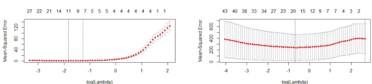
Common sense would suggest selecting a value forλthat produces the min-imum CV error, however this method is not particularly stable and fails to pro-vide optimal sparsity. Figure 2.1 propro-vides sample plots from two CV processes. In the image on the right, there is little noticeable change in the error produced by models associated withlog(λ)values between -3 and -0.5, and there is no sta-ble way to predict that the true minimum average will occur at one point along this “plateau” rather than another; in fact, a small change in the grid increment or a different seed for the random number generator may be the most notable explanation for selecting one value over another. Thus it is more advisable to implement the 1SE rule of Breiman et al. [8]: add together the minimum CV error and one standard error associated with the same model and select the λ value associated with the sparsest model with a lower CV error. This increases the stability of the prediction and tends to choose sparser models.

There are some who rely instead upon the theoretical bounds on prediction error mentioned in Section 2.2 to select the penalty parameter. Generally these bounds are only applicable if the selected λ is large enough to obtain a high probability of selecting the true active set. One such option is the so-called

“uni-versal choice” ofλ=

q

2 log(p)

n . These values obviate the need for any potentially time-consuming use of CV, however they are not as adaptable to variations in the dataset. [16] discuss a bound on the prediction error given this selection if the true active set is sufficiently small relative ton, but show that mild correla-tions can significantly decrease the rate of convergence.

Lederer and M ¨uller in [43] aptly describe the pervasiveness of methodolo-gies requiring a tuning parameter in high-dimensional variable selection pro-cedures, and the need for a “tuning parameter that is properly adjusted to all aspects of the model [which is] difficult to calibrate in practice.” They also de-cry the use of CV to select λ as “computationally inefficient” and producing “unsatisfactory variable selection performance”. The poor variable selection performance of the CV usually comes from using the model associated with the minimum RSS which tends to overfit the model; implementing the 1SE rule, while generally mitigating the under-penalization issue, vastly overcorrects in the face of unusual observations. It is important to note, however, that both CV-selection methods can be affected by even moderately influential observations.

Ryan Tibshirani and Jonathan Taylor [63] discuss ways to view the degrees of freedom of a Lasso problem in terms of the variable selection, i.e. the “effec-tive number of parameters”. They discuss choosing tuning parameters based on Mallow’sCp as a computationally-efficient alternative to CV. However, this begs the following question: how do they determine the estimated degrees of freedom? They address Stein’s Unbiased Risk Estimate (SURE) in relation to degrees of freedom, where

d f(g)= E

(∇ ·g) (y)

estimators, though, involves either knowing the model fits from the unknown model or knowing the expected value of the predictions.

2.2.1

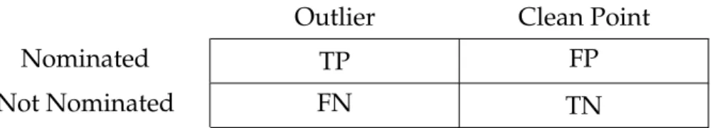
Outliers and the Penalty Parameter

Outliers can exert undue influence over the coefficient estimates and the active set selection of a Lasso fit. However, outliers also can affect the amount of spar-sity induced in the model. This influence is most notable in CV-selected penalty parameters, even in low-dimensional settings. Interestingly, the two methods of selecting an appropriate penalty parameter (i.e. the minimum and 1SE rules) appear to have opposite reactions to the presence of outliers.

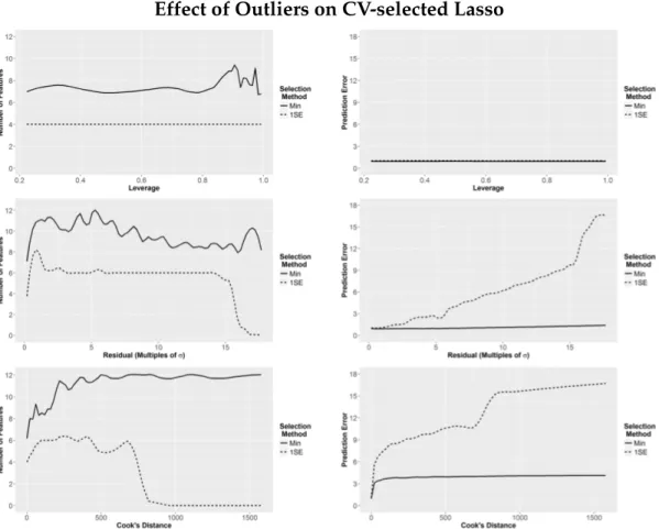
A preliminary study in order to examine the effect of outliers on the CV-selected Lasso penalty parameter involved generating a data set with 100 ob-servations on 12 Gaussian, uncorrelated predictors. The response was modeled using the standard linear equationy=Xβ+σwhereis standard normal,σ= 7, andβ= (5,−5,5,−5,0, . . . ,0)T. Figure 2.2 shows the resulting impact of taking a single observation and moving it away from the rest of the data set in either the predictor space, the residual dimension, or both. Instead of documenting the change to the penalty parameter λ which is not directly comparable between different data sets, the size of the active set and the average in-sample predic-tion error provide a clearer examinapredic-tion of the effect of the selected penalty parameter on the model fit. The in-sample error is useful (rather than the CV error) as it reflects how closely the selected model follows the outlying point.

The instability of the minimum rule is clearly evident in the additional vari-ability in the curves over the 1SE rule, especially in the residual plot (the middle

Cross-validation Plots

Figure 2.1: Plots representing the CV error for various values of λ. The dashed lines represent the minimum and 1SE selected penalty parameters. The figure on the left included only clean observations; the figure on the right with one influential point.

image in the left column of Figure 2.2). This instability is a direct result of the minimum occurring arbitrarily within the wide range of models with statisti-cally equivalent CV errors (the plateau in Figure 2.1). It is also evident that the minimum rule tends to favor less-sparse models with in order to achieve the best possible prediction accuracy, while the 1SE rule tends to exhange more in-terpretable, sparse models for some prediction accuracy. This trade-off is well-known, and should be carefully considered in the context of a given analytic goal.

In the presence of outliers, the minimum rule tends to select much larger models than if the outlying observation were to be removed. In Figure 2.1, the minimum CV error shifts far to the right with the introduction of an outlier, however the model sizes associated with eachλvalue have become significantly larger; despite the larger penalty, the minimum rule would select a model with nearly 20 predictors instead of 12. The 1SE rule, however, tends to select more sparse models due to the vast increase in the CV estimated standard errors. In the CV plots above, the largest standard error for a clean dataset had a value of approximately 20, or 15% of the estimated CV errors; with the outlier, the smallest standard error is approximately 200, or 66% of the estimated CV error.

This leads to an excessive reduction in the size of the active set selected, and tends toward a null model.

According to Figure 2.2, leverage does not appear to have much effect on the size of the active set except that the size of the model associated with the minimum rule becomes increasingly volatile ashiapproaches 1; the 1SE models are unaffected. Although it is not always evident due to the scale of the plots (which were set thusly for comparison purposes), 1SE models have consistently higher prediction errors and the prediction error becomes more volatile for both methods as leverage increases. The behavior is the same whether the leverage occurs in major or minor eigenvector directions, however the effect is more pro-nounced when along major eigenvector directions.

With a high residual outlier, the 1SE rule proves to be quite stable, select-ing the correct number of features for the model over a wide range of residual values; however if the observation is pushed sufficiently far from the model (at approximately 15σ), the penalty parameter quickly grows to force a uniform se-lection of the null model. The minimum rule model has no such dramatic drop to the null, however there does appear to be a steadily slow decline in the active set size. This persistence in a high variable selection rate is thus able to main-tain astonishingly good in-sample prediction accuracy, which is also a warning that that the model tends to follow the outlying point, despite its relatively low leverage (hi ≈ 0.25).

The most intriguing graphs in Figure 2.2 is in the selected size of the active set for influential observations. In every other occurrence, an increase in obser-vation distance was met by either a decrease in active set size or indifference, but the two methods tended to agree in the direction if not in the magnitude or

Effect of Outliers on CV-selected Lasso

Figure 2.2: Change in active set selection (left column) and average pre-diction error (right column) of CV-selected Lasso models in the presence of outliers. Uncorrelated data set withn = 100and p= 12, with a true active set of four predictors. Outliers introduced as (from top to bottom): high leverage points, high residual points, and influential points.

rapidity of the effect. Here, however, we see entirely opposite results based on the penalty parameter selection method: the 1SE rule model tends toward the null model as influence increases as before, however the minimum rule model tends toward the full model.

In higher dimensional situations, the minimum rule appears to pick increas-ingly larger models both for high residual points and influential points, though it levels out before the full model is reached. In a situation with 50 observations and 45 variables, the plot plateaued between 25 and 30 features for the mini-mum model in the presence of either high residual or influential points. The

Effect of Multicollinearity on CV-selected Lasso

Figure 2.3: Change in active set selection (left column) and average pre-diction error (right column) to CV-selected Lasso model in the presence of autoregressive multicollinearity. Data generated from a multivariate nor-mal withn=50, p=45, and an active set of size 4.

1SE model behaved in a similar manner to the low-dimensional setting, though it selected a larger number of predictors for a short time before dropping to the null model.

2.2.2

Multicollinearity and the Penalty Parameter

As correlation between predictors increases, it also appears as though cross-validation tends to select larger models in the presence of higher correlation between predictors. This trend is similar for both selection methods, with the minimum rule consistently selecting on average five more predictors than the 1SE rule.

Hebiri and Lederer [33] discuss the fact that penalty parameters based on fast-rate and slow-rate bounds (which depend only on sample size, number of parameters, and variance) tend to suffer when it comes to prediction accuracy. CV tends to work better as a method of parameter selection in the face of highly collinear predictors. This seems to be clearly exhibited in Figure 2.3, where the “universal” penalty parameterλ= 2 log(_n p)tends to under-select the model.

How-ever, as concluded in [33], even in these instances some artificial inflation of the penalty parameter (inducing greater sparsity) would improve model inter-pretability at the expense of some prediction bias.

2.3

Least Angle Regression

Consider the usual regression data structure withn× ppredictor matrixXwith columns standardized to have mean 0 and variance 1 and response vectory cen-tered at 0. The true underlying model is assumed to follow the sparse regression form

y=Xβ+σ2

where i ∼iid N(0,1) and most elements of β are zero. Let A be the active set, the set of indices of all non-zero elements of β, with cardinality |A|. There are three primary possible purposes for fitting the model: identifying the variables that are members of the active set, interpreting the coefficient estimate βˆ, and obtaining the predicted valuesyˆ =Xβˆ. The model is to be fitted according to the Lasso model discussed in Section 1.4.

The LARS algorithm described in [20] for estimating the Lasso is a (near) homotopy which introduces variables sequentially into the model. The under-lying principal is that the estimated coefficient vector is updated through an adaptive piecewise-linear function (therefore differentiable almost everywhere) on a gradually increasing subset of predictors and responses, with nodes occur-ring whenever new variables enter the model.

As penalty parameter values are generally unknown a priori, the LARS al-gorithm (as with many other Lasso estimation methods) operates in a similar

way to standard tree-building methods like CART [8]: begin with a null model and gradually add in variables until the model is “full”. This model path may then be “trimmed” to an optimal size by setting the penalty parameter to an appropriate value.

2.3.1

Geometric Motivation

The geometric idea underlying the LARS algorithm is that only those variables most correlated with the residuals should be included in the model. Imagine that the coefficient estimate vector traces out a piecewise linear path through the coordinate space parametrically indexed on the penalty fraction s ∈ [0,1] described in Section 2.2, wheres=0corresponds to the null model whereA=∅

and s = 1 corresponds to the full regression model. The regression model is considered “full” when A contains either all variable indices or there are no more available degrees of freedom (i.e. |A| = min(n− 1,p) if the intercept is estimated).

At s = 0, the path starts at the origin and begins moving along the axis of the coefficient associated with the variable which is most correlated with the response (which acts as the initial residuals, sinceymay be assumed to be cen-tered without loss of generality). At a certain point, another predictor variable yields a correlation with the corresponding residuals equal to that of the ini-tial variable. At this point the path experiences a node (or joint, or elbow) in order to introduce the new variable into the model. The path continues in a lin-ear fashion along the new “equiangular” direction (that is, the vector direction which bisects the angle between the previous coefficient trajectory and the new

axis). When another variable becomes equally correlated with the residuals cor-responding to the point along the coefficient path, the path again experiences another node and changes direction. This continues until the model is full. For instances where p<n, the coefficient vector when s=1is the OLS solution.

2.3.2

Algorithm Details

This description of the LARS algorithm relies heavily on the paper by Efron et. al. [20]. Begin by centering the response vector y, and centering and scaling the predictor matrix columns to have mean 0 and variance 1. To calculate the path, begin with a null model such that A = ∅_{, i.e.} βˆ = 0 and the residuals

e = y. Determine correlations between the residuals and each of the predictors usingCˆ = eT_{X. LetC} max = maxj cˆj

be the largest correlation in absolute value

and ˆj = arg max_j<A cˆj

be the index of the variable(s) Xˆj most correlated with

e. To update the coefficient vector estimate, it is necessary to determine the new direction of the trajectory and also the distance along this vector to travel before the next variable should enter the model. Assume that at the current node we have obtained a coefficient estimateβˆ0 with corresponding fitted valuesyˆ0, residuals e0, and correlation vector Cˆ0 through initialization or completion of the previous step.

The active setA0 =nj: ˆβ0,j ,0

o

consists of the indices of all variables that are included in the model corresponding to the current node. Begin by updating Aso thatA = nj: ˆcj =Cˆmax

o

. LetX_A be the design matrix including only those columns with indices inA, letG_A= XT

Algorithm 1:LARS Algorithm for Lasso fit Data: centeredy; centered and scaledXn×p

Result: LARS path of coefficient vectorβλ0 indexed by penalty parameter λ0

(as step or fraction) Initialize: Coefficient vectorβ=0 Active setA= ∅ Residualse=y Penaltyλ0 = ₀ while |A|<min(n,p)do C=eT_X Cmax= max cj A=n j: cj = Cmax o

Determine new coefficient direction G_A= XT_AX_A w_A= 1T AG−1A1A −1/2 G−1 A

Determine distance in new direction to next node

a=XT_X AwA. a_A= 1T_AG−1_A1_A −1/2 ˆ γ=min+_j<A ( Cmax−cj a_A−aj ,Cmax+cj a_A+aj ) Update: β e λ0

with order equal to|A|_{. The new coefficient direction is calculated by} w_A = 1T_AG−1_A1_A−

1 2

G−1_A.

The new coefficient estimates are updated using the equation ˆ

β(γ)= _βˆ_0+γwA

where γ is a scalar multiple. Now that the direction has been determined, the next step is to determine the distance (represented byγ) to the next node.

To determine this, leta = XT_X

AwA. Note thataA = 1T AG−1A 1A −12 1_A, however for convenience I will usea_A to represent the scalar1T

AG−1A1A

−12

vector form previously given. Parametric vector functions onγ can be used to represent the new fitted values

ˆ

y(γ)=yˆ0+γXAwA and the correlation vector

C(γ)=XT(y−yˆ(γ))=Cˆ0−γa

as the coefficient vector βˆ(γ) progresses along the path defined above. Note that the elements ofC(γ)belonging toAwill remain equivalent and largest (in absolute value) asγ changes. Let us call this valueC_A(γ) = Cmax−γa_A. A new variable will enter the model when some

cj(γ)

=CA(γ)with j<A. Setting the

two values equal to each other and solving forγyields the estimate ˆ γ=min j_<A +(Cmax−cj a_A−aj ,Cmax+cj a_A+aj )

wheremin+indicates that the minimum is only taken over positive arguments.

2.4

Homotopy for Sequential Observations

Standard least squares (LS) regression is known to produce better predictions when every predictor is added to the model, regardless of each predictor’s true relationship with the response. Lasso regression is one of a family of penalized regression techniques that counterbalance this tendency in order to achieve a sparser estimate. In the Lasso, a weighted`1penalty on the estimated parameter vectorβis added to the minimization problem, i.e.

ˆ

β=arg min

β kXβ−yk

2

where X is the n-by-p matrix of predictors, yis the n-dimensional vector of re-sponses, µ is a prespecified regularization parameter, and kak₁ = P

i|ai| is the `1-norm. There have been several proposed methods for solving this minimiza-tion problem. The most commonly used is the least angle regression (LARS) algorithm of Efron et. al. [20]. Garrigues & El Ghaoui [27] developed an it-erative update homotopy algorithm specifically designed for estimates where observations are received over time.

Suppose that theX˜ andy˜are the data for thenobservations that have already been received, and the coefficient vector β(n) _{and regularization parameter µn} have already been estimated. In order to update these estimates when the new observation(yn₊1,xn+1)∈R×Rp(the augmented data set is denoted asX andy), Garrigues and El Ghaoui [27] presented the new minimization equation which weights the(n+1)st _{observation byt.}

β(t, µ)=arg min β        1 2 ˜ X txT n+1 ! β− y˜ tyn₊1 ! 2 2 +µkβk₁        .

So β(n) _{= β(0, µn) is known from the first n observations, and the goal is to} obtainβ(n+1) _{= β(1, µn}

+1). Let the vectorv = sign(β(n))and the active set A = {j :

β(n)

j , 0}; matrices and vectors subscripted with 1 utilize only the columns inA. The authors propose updating the regularization parameter using

µn₊1 = n n+1µnexp 2nηxT n+1,1 X₁TX1−1v1xnT+1,1β1−yn+1 .

Fixingµ= µn+1, then looking at the wayβ(t)=β(t, µn+1)changes astvaries from 0 to 1 shows the changes that occur to the active setAby incorporating the(n+1)st observation. Theset’s can be calculated explicitly.

not inAare 0), the equation can be expressed β1(t)= β˜1− (t2_−1)¯e 1+α(t2₋₁₎u where ˜ β1 = X₁TX1 −1 X₁Ty−µv₁ ¯ e= xTn+1,1β1˜ −yn+1 u=X₁TX1 −1 xn₊1,1 α= xTn+1,1u.

The active set can change either by having a previously non-null coefficient becoming 0, or by having a 0 element become non-null. In the first scenario, the next value oftat which componentβ1i(t),i∈Abecomes 0 is at

t1i =      1+ ¯ eui ˜ β1i −α !−1      1 2 .

For the second scenario, letX2be the columns ofX not in the active set,e˜ be the(n+1)dimensional vector of residuals,cjbe the jth column ofX2, and x(j)be the jth column of xn₊1,2. The next value oft at which the jth component ofAC will joinAwhentis equal to

t2j = min                    t₂+_j =      1+ ¯ ex(j)_−cT jX1u µ−cT je˜ −α !−1      1 2 t₂−_j =      1+ ¯ ex(j)_−cT jX1u −µ−cT je˜ −α !−1      1 2 .

Then the next change to the active set will occur at t0 = _min{minit1i,_minjt 2j}. If t0

< [0,1], then incorporating the(n+1)st observation will leave Aunchanged;

otherwise, the active set will change, so the process is repeated untilt0