Estimation under cross-classified sampling with application to a childhood survey

TSE‐659

“Estimation under cross‐classified sampling with

application to a childhood survey”

Hélène Juillard, Guillaume Chauvet and Anne Ruiz‐Gazen

Estimation under cross-classified sampling with

application to a childhood survey

H´

el`

ene Juillard

Guillaume Chauvet

Anne Ruiz-Gazen

April 25, 2016

Estimation under cross-classified sampling

with application to a childhood survey

Abstract

The cross-classified sampling design consists in drawing samples from a two-dimension population, independently in each two-dimension. Such design is commonly used in consumer price index surveys and has been recently applied to draw a sample of babies in the French Longitudinal Survey on Childhood, by crossing a sample of maternity units and a sample of days. We propose to derive a general theory of estimation for this sampling design. We consider the Horvitz-Thompson estimator for a total, and show that the cross-classified design will usually result in a loss of efficiency as compared to the widespread two-stage design. We obtain the asymptotic distribution of the Horvitz-Thompson estimator, and several unbiased variance estimators. Facing the problem of possibly negative values, we propose simplified non-negative variance estimators and study their bias under a super-population model. The proposed estimators are compared for totals and ratios on

∗_{INED, 133 boulevard Davout, 75020 Paris, France}

†_{ENSAI/IRMAR, Campus de Ker Lann, 35170 Bruz, France}

simulated data. An application on real data from the French Longitudinal Survey on Childhood is also presented, and we make some recommendations. Supplementary materials are available online.

Some key words: analysis of variance, Horvitz-Thompson estimator, indepen-dence, invariance, Sen-Yates-Grundy estimator, two-stage sampling.

Short title: Estimation under cross-classified sampling

1

Introduction

The 2011 French Longitudinal Survey on Childhood ELFE (Etude Longitudinale Fran¸caise depuis l’Enfance) comprises more than 18,000 children selected on the basis of their place and date of birth. On the one hand, a sample of 320 maternity units has been drawn. On the other hand, a sample of 25 days divided in four time periods and spread across the four seasons of 2011 has been selected. The babies born at the sampled locations and on the sampled days have been approached through midwives. Data were collected on babies whose parents consented to their inclusion during their stay at the maternity unit. ELFE is conducted by the National Institute for Demographic Studies, the National Institute for Health and Medical Research and the French Blood Agency. The objective of observing children born within the same year is to analyze their physical and psychological health together with their living and environmental conditions. This large-scale study of children’s development and socialization is the first of its kind in France. The collected data are now available to public and private research teams and many projects are underway in areas such as health, health environment and social sciences. In order to derive reliable confidence intervals for finite population parameters such as totals or ratios, the ELFE sampling design has to be taken into account.

The ELFE sample is drawn according to a non-standard sampling design, called Cross-Classified Sampling (CCS), following Ohlsson (1996). It consists in drawing

independently two samples from each component of a two-dimensional population. In the ELFE survey, a sample of maternity units and a sample of days are inde-pendently selected. This sampling design appears in other contexts than the ELFE survey. Some examples include consumer price index surveys, as detailed in Dal´en & Ohlsson (1995) for the Swedish survey, where outlets and items are sampled, and business surveys (Skinner, 2015), where businesses and products are sampled. Due to its particular properties, CCS deserves a specific attention. However, as noted by Skinner (2015), ”the literature on the theory of cross-classified sampling is very limited”. In particular, no general theory is derived under the finite population framework. While the papers by Vos (1964) and Ohlsson (1996) focus on sim-ple random sampling without replacement, Skinner (2015) gives some results under stratified without replacement simple random sampling and under with replacement unequal probability sampling. Dal´en & Ohlsson (1995) provide some results under probability proportional to size without-replacement sampling.

In the present paper, we develop a general theory for estimation and variance esti-mation under CCS. The asymptotic normality of the Horvitz-Thompson estimator is derived under some mild conditions. A comparison with a two-stage sampling design is carried out in a general framework. We also raise an issue, not reported before, of possible negative values for Horvitz-Thompson and Yates-Grundy variance estimates. This problem occurs even in the simplest case of simple random sampling without replacement. Non-negative simplified variance estimators are therefore in-troduced. Conditions for their approximate unbiasedness are given under a design-based and a model-design-based approach. The properties of our variance estimators are evaluated through a small but realistic simulation study when estimating totals and ratios. Finally, an application to the ELFE data is detailed.

2

Cross-classified sampling design

2.1

Notations and Horvitz-Thompson estimation

Keeping in mind the ELFE survey, we consider a population UM of NM maternity

units and a population UD of ND days. However, the developments below are

completely general and may be applied to any populationsUM andUD. We will use

the indexes i and j for the maternity units, and the indexes k and l for the days. We consider a sampling design pM(·) on the population UM, leading to a sample

SM of (average) sizenM, and a sampling designpD(·) on the populationUD leading

to a sample SD of (average) size nD. We assume that the two samples are selected

independently. The cross-classified sampling design p(·) on the product population

U =UM ×UD is therefore defined as

p(s) = pM(sM)×pD(sD) for any s =sM ×sD ⊂UM ×UD.

Let πM

i denote the probability that i is selected in SM, πMij denote the probability

that units i and j are selected jointly in SM, and let ∆Mij = πijM −πiMπjM. The

quantitiesπD

k ,πDkland ∆Dklare similarly defined. We assume that the first and

second-order inclusion probabilities are non-negative in each population. The probability for the pairs (i, k) to be selected in the product sample SM ×SD isπiMπkD, and the

probability for the pairs (i, k) and (j, l) to be selected jointly in the product sample

SM ×SD isπijMπklD.

We are interested in some variable of interest with value Yik for the maternity unit

i and the day k. The total tY = P

i∈UM

P

k∈UDYik is then unbiasedly estimated by

the Horvitz-Thompson (HT) estimator ˆ tY = X i∈SM X k∈SD Yik πM i πkD = X i∈SM X k∈SD ˇ Yik where Yˇik = Yik πM i πkD . (2.1)

HT-estimator is VCCS ˆtY = X i,j∈UM X k,l∈UD ΓijklYˇikYˇjl (2.2)

where Γijkl =πijMπklD−πiMπjMπkDπlD. The Sen(1953)-Yates-Grundy(1953) form

VCCS ˆtY = −1 2 X (i,k)6=(j,l)∈UM×UD Γijkl Yˇik−Yˇjl 2 (2.3) can be used alternatively when both sampling designs are of fixed size.

Our set-up can be compared to the usual two-stage framework, by considering UM

as a population of Primary Sampling Units (PSUs) and UD as a population of

Secondary Sampling Units (SSUs), each maternity unit i being associated to the same population of days. In case of two-stage sampling, denoted by M D, a first-stage sample SM is selected in UM, and some second-stage samples Si are selected

independently using pD(Si) for eachi∈SM (see S¨arndal et al., 1992). The variance

of the HT-estimator is then

VM D ˆtY = V_{M D}P SU ˆtY +V_{M D}SSU ˆtY (2.4) where V_{M D}P SU ˆtY = X i,j∈UM X k,l∈UD ∆M_ij πD_kπ_lDYˇikYˇjl, (2.5) V_{M D}SSU ˆtY = X i∈UM X k,l∈UD π_iM∆D_klYˇikYˇil. (2.6)

Alternatively, we could considerUD as a population of PSUs andUM as a population

of SSUs, each day k being associated to the same population of maternity units. In this case, the variance of the HT-estimator under two-stage sampling is

VDM ˆtY = V_DMP SU ˆtY +V_DMSSU ˆtY (2.7) where V_DMP SU ˆtY = X k,l∈UD X i,j∈UM ∆D_klπM_i π_jMYˇikYˇjl, (2.8) V_DMSSU ˆtY = X k∈UD X i,j∈UM π_kD∆M_ijYˇikYˇil. (2.9)

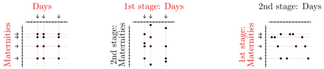
The different features of CCS and two-stage sampling on a two-dimension population are illustrated on Figure 1.

Days Maternities 1st stage: Days Maternities 2nd stage: 2nd stage: Days Maternities 1st stage:

Figure 1: Cross-classified sampling (left panel), two-stage sampling DM with pri-mary units in UD (central panel), two-stage sampling M D with primary units in

UM (right panel)

2.2

Variance decomposition for cross-classified sampling

The covariance Γijkl may be written in several ways, leading to alternative variance

decompositions. Plugging Γijkl =πDkl∆Mij +πijM∆Dkl−∆Mij∆Dkl into (2.2) gives

VCCS ˆtY = V1 tˆY +V2 ˆtY −V3 ˆtY (2.10) where V1 ˆtY = X k,l∈UD X i,j∈UM πD_kl∆M_ij YˇikYˇjl, (2.11) V2 ˆtY = X i,j∈UM X k,l∈UD πM_ij∆D_klYˇikYˇjl, (2.12) V3 ˆtY = X i,j∈UM X k,l∈UD ∆M_ij∆D_klYˇikYˇjl. (2.13)

Plugging Γijkl = ∆MijπkDπlD+ ∆klDπiMπjM + ∆Mij∆Dkl into (2.2) gives

VCCS tˆY = V_{M D}P SU ˆtY +V_DMP SU ˆtY +V₃ ˆtY (2.14) and we haveV1 ˆtY =VP SU M D ˆtY +V₃ ˆtY andV2 ˆtY =VP SU DM ˆtY +V₃ ˆtY . This second decomposition was originally derived by Dal´en & Ohlsson (1995). It is also given in Ohlsson (1996), and in equation (3) of Theorem 2.2 of Skinner (2015). Other decompositions are possible, e.g. through an analysis of variance decomposition as for two-stage sampling.

2.3

Comparison with two-stage sampling

From expressions (2.7) and (2.14), we obtain after some algebra that

VCCS ˆtY −VDM tˆY = X i,j∈UM ∆M_ij X k6=l∈UD π_klDYˇikYˇjl. (2.15)

In case of Poisson sampling (PO) inside UM and when Y is assumed to be

non-negative, the right-hand side in (2.15) is non-negative and CCS is thus less efficient than two-stage sampling. In case of fixed-size sampling inside UM, equation (2.15)

may be alternatively written as

VCCS ˆtY −VDM ˆtY = X i6=j∈UM (−∆M ij) 2 X k6=l∈UD πD kl πD kπDl Yik πM i − Yjk πM j Yil πM i − Yjl πM j . (2.16)

If the so-called Sen-Yates-Grundy conditions are respected for pM, the quantities

(−∆M

ij) are non-negative. If Yik is roughly proportional to the size of the maternity

unit i, as can be expected for count variables, the quantities

Yik πM i − Yjk πM j Yil πM i − Yjl πM j

will tend to be positive unless the inclusion probabilities π_iM are defined propor-tionally to some measure of size. CCS sampling would then be less efficient than two-stage sampling. This result is illustrated in section 4.1 on some simulated pop-ulations when both pM and pD are simple random sampling without replacement

(SI) designs, and for different sample sizes.

3

Variance estimation

3.1

Design-unbiased variance estimation

The HT variance estimator for VCCS tˆY is ˆ VHT ˆtY = X i,j∈SM X k,l∈SD Γijkl πM ij πklD ˇ YikYˇjl. (3.1)

It may be also derived from (2.10), leading to the alternative writing ˆ VHT ˆtY = Vˆ_1,HT ˆtY + ˆV_2,HT tˆY −Vˆ_3,HT tˆY (3.2) where ˆ V_1,HT ˆtY = X i,j∈SM X k,l∈SD ∆M ij πM ij ˇ YikYˇjl, (3.3) ˆ V_2,HT ˆtY = X i,j∈SM X k,l∈SD ∆D_kl πD kl ˇ YikYˇjl, (3.4) ˆ V_3,HT ˆtY = X i,j∈SM X k,l∈SD ∆M_ij πM ij ∆D kl πD kl ˇ YikYˇjl. (3.5)

If pM and pD are both Poisson sampling designs, this variance estimator is always

non-negative. Otherwise, it may take negative values even if pM and pD are both

SI designs (denoted by SI2_{) as illustrated in section 4.2. When p}

M and pD are both

fixed-size sampling designs, we may alternatively consider the Yates-Grundy like variance estimator: ˆ VY G tˆY = Vˆ_{1,Y G} ˆtY + ˆV_{2,Y G} ˆtY −Vˆ_{3,Y G} tˆY (3.6) where ˆ V_{1,Y G} ˆtY = −1 2 X i6=j∈SM ∆M ij πM ij ˆ Yi• πM i − Yˆj• πM j !2 (3.7) ˆ V_{2,Y G} ˆtY = −1 2 X k6=l∈SD ∆D_kl πD kl ˆ Y•k πD k − Yˆ•l πD l !2 (3.8) ˆ V_{3,Y G} ˆtY = −1 2 X (i,k)6=(j,l)∈SM×SD ∆M_ij∆D_kl πM ij πklD ˇ Yik−Yˇjl 2 (3.9) with ˆY•k = P i∈SM Yik/π M

i is the estimated sub-total for the day k and ˆYi• =

P

k∈SDYik/π

D

k is the estimated sub-total for the maternity unit i.

It can be proved that ˆVHT tˆY

in (3.2) and ˆVY G tˆY

in (3.6) match term by term, whenpM and pD are stratified simple random sampling (STSI) designs. In the same

Skinner (2015). This variance estimator does not match ˆVHT tˆY

or ˆVY G ˆtY

term by term, since Skinner’s variance estimator is based on the variance decomposition in equation (2.14), while our variance estimator is based on the variance decomposi-tion in equadecomposi-tion (2.10). Nevertheless, both variance estimators are globally identical in the STSI case.

Another variance estimator is obtained in Dal´en & Ohlsson (1995), in case of a probability proportional to size without-replacement sampling design in both di-mensions. Summing the variance component estimators in equations (4.1)-(4.3) of Dal´en & Ohlsson (1995) leads to a similar variance estimator than in our equa-tion (3.6), except that −Vˆ_{3,Y G} ˆtY

is replaced with + ˆV_{3,Y G} ˆtY

which results in an overestimation of the variance. This overestimation can be be neglected in cases when V3 ˆtY

is small as compared to the other variance components (see Table 1 in Section 4.2).

If both sampling designs satisfy the Sen-Yates-Grundy conditions (SYG), the terms ˆ

V_{1,Y G} ˆtY

and ˆV_{2,Y G} ˆtY

are non-negative. However, the term ˆV_{3,Y G} ˆtY

is usually non-negative, which may lead to negative values for ˆV_{Y G} ˆtY

as illustrated in the simulations of section4.2. It is thus desirable to have access to non-negative variance estimators with limited bias.

3.2

Non-negative variance estimators

We consider the variance decomposition in (2.10), and study the relative order of magnitude of the components. We make the following assumptions:

H1: There exist some constantsα1 and α2 such that

∀k ∈UD, 1 NM X i∈UM Y_ik2 ≤α1, and ∀i∈UM, 1 ND X k∈UD Y_ik2 ≤α2.

H2: There exist some constantsλ1 >0 and λ2 >0 such that ∀k∈UD, πkD ≥λ1 nD ND , and ∀i∈UM, πiM ≥λ2 nM NM .

H3: There exist some constantsγ1 and γ2 such that

∀k 6=l∈UD, N2 D nD sup k6=l∈UD ∆D_kl ≤γ1, and ∀i6=j ∈UM, N2 M nM sup i6=j∈UM ∆M_ij ≤γ2.

H4: There exists some constantδ >0 such that

VCCS ˆtY ≥ δN_M2 N_D2 1 nM + 1 nD .

It is assumed in (H1) that the variable y has bounded moments of order 2 for each maternity unit i and for each day k. Assumptions (H2) and (H3) are classical in survey sampling and are satisfied for many sampling designs, see for example Cardot et al. (2013). It is assumed in (H4) that the variance of the HT-estimator under CCS sampling has the order N2

MND2(n

−1

M +n

−1

D ). From assumptions (H1-H4), there

exist some constants C1, C2 and C3 such that

V₁ ˆtY VCCS ˆtY ≤ C1 1 1 +nMn−_D1 , (3.10) V₂ ˆtY VCCS ˆtY ≤ C2 1 1 +nDn−M1 , (3.11) V3 ˆtY VCCS ˆtY ≤ C3 1 nDn−M1+nMn−D1 (3.12) The proof is given in Appendix8. It follows from (3.10)-(3.12) that ifnD is large and

nM is bounded, bothV2 ˆtY

andV3 ˆtY

are negligible and a non-negative simplified variance estimator can be derived by focusing on V₁ ˆtY

only. This leads to ˆ VSIMP1 ˆtY = Vˆ_{1,Y G} ˆtY . (3.13)

If the sampling design pD satisfies the SYG conditions, this simplified estimator is

always non-negative. In the particular SI2 case, we obtain ˆ VSIMP1 ˆtY = N_M2 1 nM − 1 NM s2_Yˆ_◦• (3.14)

where s2_Yˆ ◦• = 1 nM −1 X i∈SM ˆ Yi•− 1 nM X j∈SM ˆ Yj• !2 . (3.15) Symmetrically, both V₁ ˆtY andV3 tˆY

may be seen as negligible ifnM is large and

nD is bounded. Another simplified variance estimator is thus

ˆ VSIMP2 ˆtY = Vˆ_{2,Y G} ˆtY . (3.16)

If the sampling design pM satisfies the SYG conditions, this estimator is

non-negative. In the particular SI2 case, we have ˆ VSIMP2 ˆtY = N_D2 1 nD − 1 ND s2_Yˆ •◦ (3.17) where s2_Yˆ •◦ = 1 nD −1 X k∈SD ˆ Y•k− 1 nD X l∈SD ˆ Y•l !2 . (3.18)

A third possible simplified variance estimator is ˆ VSIMP3 tˆY = VˆSIMP1+ ˆVSIMP2 = Vˆ_{1,Y G} ˆtY + ˆV_{2,Y G} ˆtY . (3.19)

This estimator is non-negative if both pD and pM satisfy the SYG conditions. It is

approximately unbiased for VCCS tˆY

ifnD is large and nM is bounded, or if nM is

large and nD is bounded. In the particular SI2 case

ˆ VSIMP3 ˆtY =N_M2 1 nM − 1 NM s2_Yˆ ◦• +N 2 D 1 nD − 1 ND s2_Yˆ •◦. (3.20)

Similar formula can be easily derived in the case of stratified simple random sampling without replacement and will be used in Section 5.

3.3

Relative bias under a superpopulation model

We consider the following superpopulation model

Yik =µ+σMUi+σDVk+σEWik (3.21)

where Ui, Vk and Wik are independently generated according to a standard normal

distribution. This is a particular case for a single stratum of the stratified cross-classified population model introduced in equation (8) of Skinner (2015), where the fixed and random effects are allowed to depend on the strata. Model (3.21) is an analysis of variance model with two crossed random factors and without repetition. Let “Em” denote the expectation with respect to the model (3.21) and “Ep”

de-note the expectation with respect to the CCS design. For each simplified variance estimator ˆVSIMPi, i = 1,2,3, the relative bias RB under the model and under the

sampling design is defined by

RBm,p h ˆ VSIMPi ˆtY i = Em n Ep h ˆ VSIMPi ˆtY i −VCCS ˆtY o Em VCCS tˆY . (3.22)

In the SI2 case, these relative biases are of the form

RBm,p h ˆ VSIMPi ˆtY i = −1/(1 +Ai) (3.23)

for i= 1 and 2 and

RBm,p h ˆ VSIMP3 ˆtY i = 1/(1 +A3) (3.24)

for some positive constant Ai, i = 1,2,3, depending on σM, σD, σE and nM, NM,

nD andND, see equations (3.25)-(3.27). Equations (3.23) and (3.24) imply that the

two first simplified variance estimators are negatively biased while the third one is positively biased. Using the notations rM = σM2 /σE2, rD = σD2/σ2E, fM = nM/NM

and fD =nD/ND, we have A1 = 1−fM 1−fD nDrM + 1 nMrD +fM , (3.25) A2 = 1−fD 1−fM nMrD + 1 nDrM +fD , (3.26) A3 = nDrM +fD 1−fD + nMrD +fM 1−fM . (3.27)

The bias of ˆVSIMP1 increases from−1 to 0 whenA1 increases, which occurs in

partic-ular when the ratio rM or the sample size nD increases. In other words, ˆVSIMP1 will

have a small bias under model (3.21) if the variable of interest contains some ma-ternity unit effect or if the number of sampled days is large enough. Symmetrically,

ˆ

VSIMP2 will have a small bias under model (3.21) if the variable of interest contains

some day effect or if the number of sampled maternity units is large enough. The bias of ˆVSIMP3 decreases from 1 to 0 when A3 increases, which occurs in particular

when rM or rD increases, or when nM or nD increases. In other words, ˆVSIMP3 will

have a small bias under model (3.21) if the variable of interest contains some ma-ternity unit or some day effect, or if the number of sampled days or the number of sampled maternity units is large enough. The simulation study in section4supports these results, and confirms that the variance tends to be underestimated with ˆVSIMP1

or ˆVSIMP2, and overestimated with ˆVSIMP3.

3.4

A central-limit theorem

To produce confidence intervals with appropriate asymptotic coverage, it is of inter-est to state a central-limit theorem (CLT) for CCS. Roughly speaking, Theorem 1 below states that if the HT-estimator follows a CLT under both sampling designs

pD and pM, then the HT-estimator also follows a CLT under CCS. It is derived

almost directly from Theorem 2 in Chen and Rao (2007), and the proof is therefore omitted.

H5: σ₁−1V1 →L N(0,1), where →L stands for the convergence in distribution under

the sampling-design, with V1 = 1 N X i∈SM Yi• πM i − X i∈UM Yi• ! and σ2₁ =V(V1) (3.28) where Yi• =P_k∈UDYik.

H6: sup_t|P(σ−₂1U1 ≤t|SM)−Φ(t)|=op(1), where Φis the cumulative distribution

function of the standard normal distribution, and where U1 = 1 N X i∈SM 1 πM i ( ˆYi•−Yi•) and σ22 =V(U1|SM). (3.29)

H7: σ₁2/σ2₂ →P γ2, where →P stands for the convergence in probability under the

sampling-design. Then N−1_(ˆt Y −tY) p σ2 1 +σ22 →L N(0,1). (3.30)

For illustration, we consider the particular case whenpD andpM are both SI designs.

Suppose that (H2)-(H4) hold, and that (H1) is strengthened to H1b: There exists δ >0 and some constantsα1 and α2 such that

∀k ∈UD 1 NM X i∈UM Y_ik2+δ ≤α1, and ∀i∈UM 1 ND X k∈UD Y_ik2+δ ≤α2.

Then by using the CLT in Hajek (1961), the assumption (H5) can be shown to hold. By mimicking the proof of Lemma 2 in Chen and Rao (1997), the assumption (H6) can be shown to hold as well.

4

Simulations

In this Section, two artificial populations are first generated using the superpop-ulation model (3.21). In Section 4.1, CCS is compared with two stage sampling

in terms of variance, which illustrates the results in Section 2.3. A Monte Carlo experiment is then presented in Section 4.2, and the variance estimators introduced in Section 3 are compared for the estimation of a total. Some attention is paid to the issue of negative values for the unbiased variance estimator. In Section 4.3, two other populations with two variables of interest for each are generated. We focus on variance estimation for a ratio, making use of the variance estimators introduced in Section3with estimated linearized variables instead of the variable of interest. The results from Tables 1 and 2 are readily reproducible using the R code provided in the supplementary materials of the present paper.

4.1

Comparison with two-stage sampling

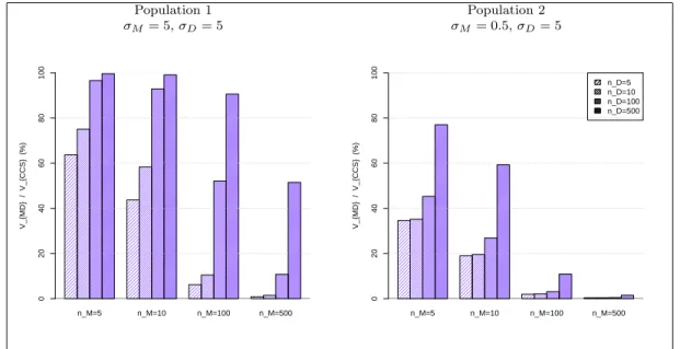
Two populations are generated according to model (3.21), with NM = 1000

mater-nity units and ND = 1000 days for each population, and with µ= 200 and σE = 5.

Equal random effects standard deviations σM = σD = 5 are used for population

1, while we use σM = 0.5 and σD = 5 for population 2. For each population, the

SI2 sampling design is used, with sample sizes, nM and nD, equal to 5, 10, 100 and

500. The ratios VM D/VCCS between the variance under two-stage sampling and the

variance under CCS are computed, and plotted as a percentage on Figure 2. A ra-tio smaller than 100 indicates that two-stage sampling is more accurate than CCS, which holds true in all cases considered in our experiment.

The ratio increases with nD and decreases when nM increases. Also, it can be

observed that the ratio decreases withσM. This impact of the maternity unit effect

is noticeable, and illustrates the substantial loss in accuracy induced by using a CCS instead of a two-stage sampling design if the maternity unit effect is small. Similar conclusions could be derived when computing the ratio VDM/VCCS.

Population 1 Population 2 σM= 5,σD= 5 σM = 0.5,σD= 5 n_M=5 n_M=10 n_M=100 n_M=500 V_{MD} / V_{CCS} (%) 0 20 40 60 80 100 n_M=5 n_M=10 n_M=100 n_M=500 V_{MD} / V_{CCS} (%) 0 20 40 60 80 100 n_D=5 n_D=10 n_D=100 n_D=500

Figure 2: VM D/VCCS ( % ) for population 1 (left panel) and population 2 (right

panel)

4.2

Variance estimation for a total

We consider the two artificial populations generated as described in Section 4.1. For each population, the SI2 sampling design is used, with sample sizes equal to 5, 10, 100 and 500, and the sample selection is repeated B = 10,000 times. For each sample b = 1, . . . , B, we compute the estimate ˆt(_Yb) of the total tY. The unbiased

variance estimator ˆV(b) and the simplified variance estimators ˆV_SIMP1(b) , ˆV_SIMP2(b) , ˆV_SIMP3(b)

are also computed for ˆt(_Yb).

For each variance estimator ˆV, we compute the Monte Carlo Percent Relative Bias

RB_mc( ˆV) = 100× B

−1PB

b=1Vˆ

(b)_−V

V ,

where the true variance V was approximated through an independent set of 50,000 simulations. The number (#NEG) of negative variance estimators ˆV(b) _{is also}

com-puted.

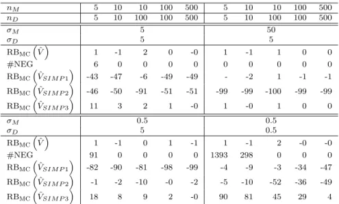
The results are reported in Table 1. The variance estimator ˆV is almost unbiased in all situations, as expected. However, this variance estimator is prone to negative values with small sample sizes when the value of σM and/or the value of σD is small

as compared to σE. The problem vanishes when the sample sizes increase. We now

turn to the simplified variance estimators. The relative bias of ˆVSIMP1decreases when

nD increases or when nM decreases, and when σM increases or when σD decreases.

This supports the findings in Section3.3. Symmetrical conclusions are drawn for the relative bias of ˆVSIMP2. Turning to ˆVSIMP3, we note that the relative bias decreases

when either σM or σD increases. This variance estimator is therefore advisable in

all cases but those where there is no maternity unit nor day effect.

nM 5 10 10 100 500 5 10 10 100 500 nD 5 10 100 100 500 5 10 100 100 500 σM 5 50 σD 5 5 RB_mcVˆ 1 -1 2 0 -0 1 -1 1 0 0 #NEG 6 0 0 0 0 0 0 0 0 0 RB_mc ˆ VSIM P1 -43 -47 -6 -49 -49 - -2 1 -1 -1 RB_mcVˆSIM P2 -46 -50 -91 -51 -51 -99 -99 -100 -99 -99 RB_mcVˆSIM P3 11 3 2 1 -0 1 -0 1 0 0 σM 0.5 0.5 σD 5 0.5 RB_mcVˆ 1 -1 0 1 -1 1 -1 2 -0 -0 #NEG 91 0 0 0 0 1393 298 0 0 0 RB_mc ˆ VSIM P1 -82 -90 -81 -98 -99 -4 -9 -3 -34 -47 RB_mcVˆSIM P2 -1 -2 -10 -0 -2 -5 -10 -52 -36 -49 RB_mc ˆ VSIM P3 18 8 9 2 -0 90 81 45 29 4

Table 1: Comparison between variance estimators for a total

4.3

Variance estimation for a ratio

We now consider variance estimation for a ratio. Two populations are generated with NM = 1000 maternity units and ND = 1000 days. In each population, two

count variables are generated so as to mimic the data encountered in the ELFE survey. More precisely, we first generate an auxiliary variable Zik according to

model (3.21) with µ = 200, σE = σD = 5, and σM = 5 or 50. The first variable

of interest Xik is generated according to a Poisson distribution with parameter Zik.

The second variable of interest Yik is generated according to a binomial distribution

pik = 0.3; (ii) unequal probabilities with logit(pik) = βZik, where β was chosen so

that the average probability is approximately 0.3. Note that Yik follows a Poisson

distribution with parameter pikZik.

The reason for this generating process is that some variable of interest Xik, like

the number of births in the ELFE survey, may contain some maternity unit and/or day effect which is reflected in the way Zik is generated. On the other hand, some

maternity unit and/or day effect may also be contained in some other variable of interest Yik, like the number of births per caesarean. Such effects may be either

similar to those for Xik like with pattern (i), or may occur differently like with

pattern (ii).

For each population, the SI2 sampling design is used, with sample sizes equal to 5, 10, 100 and 500, and the sample selection is repeated B = 10,000 times. For each sample b = 1, . . . , B, we compute the substitution estimator ˆR(b) _{= ˆt}(b)

Y /ˆt

(b)

X of the

ratioR =tY/tX. The variance estimator ˆV(b)and the simplified variance estimators

ˆ

V_SIMP1(b) , ˆV_SIMP2(b) , ˆV_SIMP3(b) are also computed for ˆt(_Yb), where the variable of interestYik

is replaced with the estimated linearized variable of the ratio.

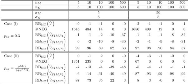
The results are reported in Table 2. The variance estimator ˆV is almost unbiased in all situations, as expected, but is prone to negative values even when the maternity unit or day effect is small. We now turn to the relative bias for the simplified variance estimators. With pattern (i), the situation is much different from that when a total is estimated, since the relative bias of ˆVSIMP3 is much larger than for the other two

simplified estimators. This can be explained as follows: when the probabilities pik

are uniform, both Yik and Xik contain the same maternity unit and day effect, but

these effects wear off in the linearized variable. Whatever the values of σM and

σD are, the situation is therefore comparable to that observed in the bottom right

cell of Table 1. With pattern (ii), the probabilities pik depend on i and k, leading

variable. In such situation, which seems more realistic in practice, the relative bias of ˆVSIMP1 and ˆVSIMP2 increase when σM or σD increase, while the relative bias of

ˆ VSIMP3 decreases. nM 5 10 10 100 500 5 10 10 100 500 nD 5 10 100 100 500 5 10 100 100 500 σM 5 50 σD 5 5 Case (i) RB_mc ˆ V -0 -1 -1 0 -0 -2 -1 -1 0 1 pik= 0.3 #NEG 1645 484 14 0 0 1656 499 12 0 0 RB_mcVˆSIM P1 -1 -1 -2 -10 -37 -1 -1 -1 -8 -32 RB_mcVˆSIM P2 0 -2 -10 -8 -30 -2 -1 -9 -8 -31 RB_mcVˆSIM P3 99 96 89 82 33 97 98 90 84 37 Case (ii) RB_mc ˆ V 0 -1 2 0 -0 -4 -3 -1 -0 0 pik= e βZik 1+eβZik #NEG 1351 235 0 0 0 67 0 0 0 0 RB_mcVˆSIM P1 -7 -13 -4 -39 -48 -5 -4 -1 -1 -1 RB_mc ˆ VSIM P2 -6 -14 -61 -40 -49 -87 -93 -99 -98 -99 RB_mcVˆSIM P3 87 73 35 22 3 8 3 -0 0 0

Table 2: Comparison between variance estimators for a ratio

5

Application to the ELFE survey

ELFE is the first longitudinal study of its kind in France, tracking children from birth to adulthood (Pirus et al., 2010). This cohort comprises more than 18,000 children whose parents consented to their inclusion. The population of inference consists of babies born during 2011 in French maternity units, excluding very premature infants. This is a two-dimensional population with 544 maternity units as spatial units and 365 days as time units. The crossing of one day and one maternity unit represents a cluster of infants.

The sample is obtained by CCS, where days and maternity units are selected in-dependently with selected families surveyed shortly after birth in 320 metropolitan maternity units and during 25 days for one year. The population of maternity units is divided into five strata of equal size. The allocation per stratum is proportional to the number of deliveries recorded in 2008. The sample selection for maternity units is stratified systematic sampling, which can be approximated by stratified simple

random sampling (STSI). The sample selection of days is not actually random, due to logistic constraints. A number of nD = 25 days is selected during 4 waves, each

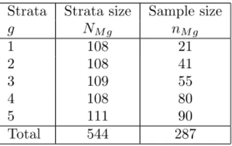
wave covering a season. It may be approximated by STSI, with four strata asso-ciated to the four seasons of 2011. The sample sizes inside strata are provided in Tables 3and 4.

Strata Strata size Sample size

g NM g nM g 1 108 21 2 108 41 3 109 55 4 108 80 5 111 90 Total 544 287

Table 3: Population and sample strata sizes for the maternity units designpM.

Strata Strata size Sample size

h NDh nDh 1 91 4 2 91 6 3 91 7 4 92 8 Total 365 25

Table 4: Population and sample strata sizes for the days design pD.

In this Section, we aim at illustrating the results previously obtained on a real data set. Some aspects of the ELFE survey, like the non-response issue or the calibration step, deserve a specific attention but are beyond the scope of the present paper and are therefore not considered. In particular, the ELFE survey is prone to several levels of non-response, since some sampled maternity units and some families refused to participate either for some specific days or for the whole period. In the present study, the sample of respondents is viewed as the original sample and in particular, we consider only the 287 maternity units that participate during the 25 days of survey. The calibration step is not taken into account. The results below are meant

to illustrate our theoretical results, but are not intended for use in other contexts. We consider seven count variables from the ELFE survey. Some of them depend on the characteristics of the maternity units (e.g., the spatial location), like the variable indicating whether the mother is followed by a midwife. Others are related to the days of the survey, like the variable indicating whether the birth occurred by caesarean. For each variable, the estimated total ˆtY from equation (2.1), the

estimated variance ˆV ˆtY

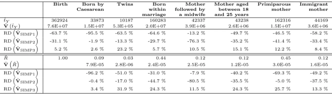
from equation (3.2) and the three simplified estimators are given in the upper part of Table 5. Similar indicators are given in the bottom part of Table 5for ratios, when the totals of the variables of interest are divided by the total number of births.

Birth Born by Twins Born Mother Mother aged Primiparous Immigrant Caesarean within followed by between 18 mother mother

marriage a midwife and 25 years

ˆ

tY 362924 33873 10187 160283 42337 43238 162316 44169

ˆ

V ˆtY 7.6E+07 1.5E+07 5.3E+05 2.0E+07 3.9E+06 2.6E+06 1.5E+07 3.6E+06

RDVˆSIMP1 -63.7 % -95.5 % -63.5 % -64.6 % -13.2 % -49.7 % -46.5 % -58.2 % RDVˆSIMP2 -31.1 % -1.9 % -13.3 % -29.7 % -76.3 % -35.2 % -41.4 % -33.4 % RDVˆSIMP3 5.2 % 2.6 % 23.2 % 5.7 % 10.5 % 15.1 % 12.2 % 8.4 % ˆ R 1.00 0.09 0.03 0.44 0.12 0.12 0.45 0.12 ˆ

VRˆ 7.9E-05 2.8E-06 2.4E-05 2.5E-05 1.2E-05 3.0E-05 1.6E-05 RD ˆ VSIMP1 -96.2 % -51.0 % -31.0 % -7.9 % -40.2 % -69.3 % -49.2 % RDVˆSIMP2 -0.4 % -17.0 % -44.7 % -80.5 % -35.5 % -5.0 % -37.5 % RDVˆSIMP3 3.4 % 31.9 % 24.3 % 11.5 % 24.3 % 25.7 % 13.3 %

Table 5: Variance estimates of estimated total and ratio on some ELFE variables

The relative difference RD between ˆVSIMP and the unbiased estimator ˆV is

RD = ˆ VSIMP tˆY ? −Vˆ tˆY ? ˆ V tˆY ? .

Different behaviours may be observed for the variables of interest, depending on the maternity unit/day effect. For instance, the variable indicating whether the birth occurred by caesarean contains an important day effect, and the RD of ˆVSIMP2 is

therefore small while that of ˆVSIMP1 is large. Symmetrically, the variable indicating

whether the mother is followed by a midwife contains a small day effect as compared to the maternity unit effect, and the RD of ˆVSIMP2 is therefore large while that of

ˆ

VSIMP1 is small. Also, we note that the RD of ˆVSIMP3 is relatively stable for all

third simplified estimator. We note however that the absolute RD of ˆVSIMP3 can be

large when estimating a ratio, which confirms the simulation results.

6

Conclusion

The present paper derives some general estimation theory for the cross-classified sampling design which was used in the recent ELFE survey on childhood. The issue of possibly negative variance estimates may arise even in case of simple random sam-pling without replacement. Alternative estimators to the usual Horvitz-Thompson and Yates-Grundy variance estimators are thus proposed, and proved to be non-negative under the usual Sen-Yates-Grundy conditions. The relative bias of the proposed variance estimators is derived for a superpopulation model. The behavior of these estimators is also investigated for totals and ratios on simulated data and on data extracted from the ELFE survey. Among the proposals, one variance estimator that leads to a slight overestimation of the variance in many cases, appears to be advisable.

Despite the present results and the recent paper by Skinner (2015), the cross-classified sampling design still deserves some attention. In particular, the treatment of non-response and the calibration problem should also be taken into account, and is currently under investigation.

7

Bibliography

Cardot, H., and Goga, C. and Lardin, P. (2013). Uniform convergence and asymp-totic confidence bands for model-assisted estimators of the mean of sampled func-tional data. Electronic Journal of Statistics, 7, 562-596.

designs. Statistica Sinica, 17, 1047-1064.

Dal´en, J. and Ohlsson, E. (1995). Variance Estimation in the Swedish Consumer Price Index. Journal of Business & Economic Statistics, 13, No.3, 347-356.

Hajek, J. (1961). Some extensions of the Wald-Wolfowitz-Noether theorem. The Annals of Mathematical Statistics, 32, 506-523.

Ohlsson, E. (1996). Cross-Classified Sampling. Journal of Official Statistics, 12, No.3, 241-251.

Pirus, C., Bois, C., Dufourg, M.N., Lano¨e, J.L., Vandentorren, S., Leridon, H. and the Elfe team (2010). Constructing a Cohort: Experience with the French Elfe Project. Population, 65, No.4, 637-670.

S¨arndal, C.-E., Swensson, B. and Wretman, J.H. (1992). Model Assisted Survey Sampling. New-York, Springer-Verlag.

Sen, A.R. (1953). On the estimate of the variance in sampling with varying proba-bilities. Journal of the Indian Society of Agricultural Statistics, 5, 119-127.

Skinner, C.J. (2015). Cross-classified sampling: some estimation theory. Statistics and Probability Letters, 104, 163-168.

Vos, J. W. E. (1964). Sampling in space and time. Review of the International Statistical Institute, 32, No. 3, 226-241.

Yates, F. and Grundy, P.M. (1953). Selection without replacement from within strata with probability proportional to size. Journal of the Royal Statistical Society B, 15, 235-261.

8

Appendix

Proof of equations (

3.10

)-(

3.12

)

From assumptions (H1), (H2) (H3) and Cauchy-Schwarz inequality, there exists some constant C such that for any k∈UD,

V( ˆY•k) ≤ C

N_M2 nM

. (8.3)

Also, from the Cauchy-Schwarz inequality, there exists some constant C such that for any k 6=l∈UD: Cov( ˆY•k,Yˆ•l) ≤ C N2 M nM . (8.4)

From equation (8.3) and assumption (H2), the first term in the right hand sum of (8.1) isO(N2

DNM2 n

−1

Mn

−1

D ). From equation (8.4) and assumptions (H2) and (H3), the

absolute value of the second term in the RHS of (8.1) isO(N2

DNM2 n

−1

M). Therefore,

there exists some constant C such that

V1 ˆtY ≤ CN 2 DNM2 nM . (8.5)

We can prove similarly that there exists some constant C such that

V2 ˆtY ≤ CN 2 DNM2 nD . (8.6)

From equation (2.13), the term V3 tˆY

may be split into four terms according to the intersection of{i, j} and{k, l}. From assumptions (H1)-(H3), it is easily shown that the absolute value of each of these four terms is O(N2

DNM2 n

−1

Mn

−1

D ). Therefore,

there exists some constant C such that

V3 ˆtY ≤ CN 2 DNM2 nMnD . (8.7)

Equations (3.10)-(3.12) follow immediately from equations (8.5)-(8.7) and assump-tion (H4).