Understanding Big Data Spectral Clustering
Romain Couillet, Florent Benaych-Georges
To cite this version:
Romain Couillet, Florent Benaych-Georges. Understanding Big Data Spectral Clustering. 2015
IEEE 6th International Workshop on Computational Advances in Multi-Sensor Adaptive
Pro-cessing (CAMSAP), Dec 2015, Cancun, Mexico. 2015.
<
hal-01205208
>
HAL Id: hal-01205208
https://hal.archives-ouvertes.fr/hal-01205208
Submitted on 25 Sep 2015
HAL
is a multi-disciplinary open access
archive for the deposit and dissemination of
sci-entific research documents, whether they are
pub-lished or not.
The documents may come from
teaching and research institutions in France or
abroad, or from public or private research centers.
L’archive ouverte pluridisciplinaire
HAL
, est
destin´
ee au d´
epˆ
ot et `
a la diffusion de documents
scientifiques de niveau recherche, publi´
es ou non,
´
emanant des ´
etablissements d’enseignement et de
recherche fran¸
cais ou ´
etrangers, des laboratoires
publics ou priv´
es.
Understanding Big Data Spectral Clustering
Romain Couillet
∗, Florent Benaych-Georges
†∗
CentraleSup´elec – LSS – Universit´e ParisSud, Gif sur Yvette, France
†MAP 5, UMR CNRS 8145 – Universit´e Paris Descartes, Paris, France.
Abstract—This article introduces an original approach to understand the behavior of standard kernel spectral clustering algorithms (such as the Ng–Jordan–Weiss method) for large dimensional datasets. Precisely, using advanced methods from the field of random matrix theory and assuming Gaussian data vectors, we show that the Laplacian of the kernel matrix can asymptotically be well approximated by an analytically tractable equivalent random matrix. The study of the latter unveils the mechanisms into play and in particular the impact of the choice of the kernel function and some theoretical limits of the method. Despite our Gaussian assumption, we also observe that the predicted theoretical behavior is a close match to that experienced on real datasets (taken from the MNIST database).1
I. INTRODUCTION
Letting x1, . . . , xn ∈Rp be ndata vectors, kernel spectral
clustering consists in a variety of algorithms designed to cluster these data in an unsupervised manner by retrieving information from the leading eigenvectors of (a possibly mod-ified version of) the so-called kernel matrix K={Kij}ni,j=1 with e.g.,Kij=f(kxi−xjk/p)for some (usually decreasing)
f : R+ → R+. There are multiple reasons (see e.g., [1]) to expect that the aforementioned eigenvectors contain information about the optimal data clustering. One of the most prominent of those was put forward by Ng–Jordan–Weiss in [2] who notice that, if the data are ideally well split inkclasses
C1, . . . ,Ckthat ensuref(kxi−xjk/p) = 0if and only ifxiand
xj belong to distinct classes, then the eigenvectors associated
with the k−1 smallest eigenvalues of In −D−
1
2KD−12,
D , D(K1n), live in the span of the canonical class-wise
basis vectors. In the non-trivial case where such a separatingf
does not exist, one would thus expect the leading eigenvectors to be instead perturbed versions of indicator vectors. We shall precisely study the matrix In−D−
1 2KD−
1
2 in this article. Nonetheless, despite this conspicuous argument, very little is known about the performance of kernel spectral clustering in actual working conditions. In particular, to the authors’ knowledge, there exists no contribution addressing the case of arbitrary p and n. In this article, we propose a new approach consisting in assuming that both pandnare large, and exploiting recent results from random matrix theory. Our method is inspired by [3] which studies the asymptotic distribution of the eigenvalues of K for i.i.d. vectors xi. We
generalize here [3] by assuming that the xi’s are drawn from
a mixture ofkGaussian vectors having meansµ1, . . . , µkand
covariances C1, . . . , Ck. We then go further by studying the
resulting model and showing that L = D−12KD− 1
2 can be
1Couillet’s work is supported by RMT4GRAPH (ANR-14-CE28-0006).
approximated by a matrix of the so-called spiked model type [4], [5], that is a matrix with clustered eigenvalues and a few isolated outliers. Among other results, our main findings are:
• in the largen, p regime, only a very local aspect of the
kernel function really matters for clustering;
• there exists a critical growth regime (with p and n) of the µi’s and Ci’s for which spectral clustering leads to
non-trivial misclustering probability;
• we precisely analyze elementary toy models, in which the number of exploitable eigenvectors and the influence of the kernel function may vary significantly.
On top of these theoretical findings, we shall observe that, quite unexpectedly, the kernel spectral algorithms be-have similar to our theoretical findings on real datasets. We precisely see that clustering performed upon a subset of the MNIST (handwritten figures) database behaves as though the vectorized images were extracted from a Gaussian mixture.
Notations:The normk · kstands for the Euclidean norm for
vectors and operator norm for matrices. The vector1m∈Rm
stands for the vector filled with ones. The operator D(v) =
D({va}ka=1) is the diagonal matrix having v1, . . . , vk (scalar
or vectors) down its diagonal. The Dirac mass at x is δx.
Almost sure convergence is denoted−→a.s., and convergence in distribution−→D .
II. MODEL ANDTHEORETICALRESULTS
Let x1, . . . , xn ∈ Rp be independent vectors with
xn1+···+n`−1+1, . . . , xn1+···+n` ∈ C` for each `∈ {1, . . . , k},
wheren0= 0andn1+· · ·+nk =n. ClassCa encompasses
data xi = µa+wi for some µa ∈Rp and wi ∼ N(0, Ca),
withCa ∈Rp×p nonnegative definite.
We shall consider the large dimensional regime where both
n andp grow simultaneously large. In this regime, we shall require the µi’s and Ci’s to behave in a precise manner.
As a matter of fact, we may state as a first result that the following set of assumptions forms the exact regime under which spectral clustering is a non trivial problem.
Assumption 1 (Growth Rate): As n → ∞, np → c0 > 0,
na
n →ca >0 (we will writec= [c1, . . . , ck]
T). Besides, 1) Forµ◦,Pk a=1 na nµa andµ◦a =µa−µ◦,kµ◦ak=O(1) 2) For C◦ , Pk a=1 na nCa and Ca◦ = Ca−C◦, kCak = O(1)andtrCa◦=O(√n). 3) Asp→ ∞, 2ptrC◦→τ >0.
The valueτis important since 1pkxi−xjk2 a .s.
−→τuniformly oni6=j in{1, . . . , n}.
We now define the kernel function as follows.
Assumption 2 (Kernel function): Function f is three-times
continuously differentiable around τ andf(τ)>0. Having defined f, we introduce the kernel matrix as
K, f 1 pkxi−xjk 2 n i,j=1 .
From the previous remark on τ, note that all non-diagonal elements of K tend to f(τ) and thus K can be point-wise developed using a Taylor expansion. However, our interest is on (a slightly modified form of) the Laplacian matrix
L,nD−12KD− 1 2
where D = D(K1n) is usually referred to as the degree
matrix. Under Assumption 1,Lis essentially a rank-one matrix with D121n for leading eigenvector (with n for eigenvalue). To avoid technical difficulties, we shall study the equivalent matrix2 L0,nD−12KD− 1 2 −nD 1 21n1T nD 1 2 1T nD1n (1) which we shall show to have all its eigenvalues of orderO(1). Our main technical result shows that there is a matrix Lˆ0
such that kL0 −Lˆ0k −→a.s. 0, where Lˆ0 follows a tractable random matrix model. Before introducing the latter, we need the following fundamental deterministic element notations3
M ,[µ◦1, . . . , µ◦k]∈Rp×k t, 1 √ ptrC ◦ a k a=1 ∈Rk T , 1 ptrC ◦ aC ◦ b k a,b=1 ∈Rk×k J ,[j1, . . . , jk]∈Rn×k P ,In− 1 n1n1 T n∈R n×n
whereja∈Rn is the canonical vector of classCa, defined by
(ja)i =δxi∈Ca, and the random element notations W ,[w1, . . . , wn]∈Rp×n Φ, √1 pW TM ∈ Rn×k ψ, 1 p kwik2−E[kwik2] n i=1∈R n.
Theorem 1 (Random Matrix Equivalent):Let Assumptions 1
and 2 hold and L0 be defined by (1). Then, as n→ ∞,
L 0−Lˆ0 a.s. −→0
2It is clearly equivalent to studyL0 orLthat have the same
eigenvalue-eigenvector pairs but for the pair (n, D121n)ofLturned into(0, D121n)
forL0.
3CapitalMstands here formeanswhilet,Taccount for vector and matrix
oftraces,P for a projection matrix (onto the orthogonal of1n1T n). whereLˆ0 is given by ˆ L0, −2f 0(τ) f(τ) P WTW P p +U BU T +2f 0(τ) f(τ) F(τ)In withF(τ) = f(0)−2ff(τ0()+τ)τ f0(τ) and U , 1 √ pJ,Φ, ψ B, B11 Ik−1kcT 5f0(τ) 8f(τ) − f00(τ) 2f0(τ) t Ik−c1Tk 0k×k 0k×1 5f0(τ) 8f(τ) − f00(τ) 2f0(τ) tT 0 1×k 5f 0(τ) 8f(τ) − f00(τ) 2f0(τ) B11=MTM + 5f0(τ) 8f(τ) − f00(τ) 2f0(τ) ttT−f 00(τ) f0(τ)T+ p nF(τ)1k1 T k
and the casef0(τ) = 0is obtained by extension by continuity (in the limitf0(τ)B being well defined asf0(τ)→0).
From a mathematical standpoint, excluding the identity matrix, when f0(τ)6= 0, Lˆ0 follows a spiked random matrix model, that is its eigenvalues congregate in bulks but for a few isolated eigenvalues, the eigenvectors of which align to some extent to the eigenvectors ofU BUT. When f0(τ) = 0,
ˆ
L0 is merely a small rank matrix. In both cases, the isolated eigenvalue-eigenvector pairs ofLˆ0 are amenable to analysis.
From a practical aspect, note that U is notably constituted by the vectors ja, while B contains the information about
the inter-class mean deviations through M, and about the inter-class covariance deviations through t and T. As such, the aforementioned isolated eigenvalue-eigenvector pairs are expected to correlate to the canonical class basisJ and all the more so thatM,t,T have sufficiently strong norm.
From the point of view of the kernel functionf, note that, if f0(τ) = 0, then M vanishes from the expression of Lˆ0, thus not allowing spectral clustering to rely on differences in means. Similarly, if f00(τ) = 0, then T vanishes, and thus differences in “shape” between the covariance matrices cannot be discriminated upon. Finally, if 58ff0((ττ))= 2ff000((ττ)), then
differences in covariance traces are seemingly not exploitable. Before introducing our main results, we need the following technical assumption which ensures that 1pP WTW P does not in general produce itself isolated eigenvalues (and thus, that the isolated eigenvalues of Lˆ0 are solely due toU BUT).
Assumption 3 (Spike control): With λ1(Ca) ≥ . . . ≥
λp(Ca) the eigenvalues of Ca, for each a, as n → ∞,
1
p
Pp
i=1δλi(Ca)
D
−→νa, with supportsupp(νa), and
max
1≤i≤pdist(λi(Ca),supp(νa))→0.
Theorem 2 (Isolated eigenvalues4): Let Assumptions 1–3
hold and define, forz∈R, the k×k matrix
Gz=h(τ, z)Ik+Dτ,zΓz
where h(τ, z) = 1 + 5f0(τ) 8f(τ) − f00(τ) 2f0(τ) k X i=1 cigi(z) 2 ptrC 2 i Dτ,z =h(τ, z)MT Ip+ k X j=1 cjgj(z)Cj −1 M −h(τ, z)f 00(τ) f0(τ)T+ 5f0(τ) 8f(τ) − f00(τ) 2f0(τ) ttT Γz=D {caga(z)}ka=1− ( caga(z)cbgb(z) Pk i=1cigi(z) )k a,b=1 andg1(z), . . . , gk(z)are, for well chosenz, the unique
solu-tions to the system 1 c0 1 ga(z) =−z+1 ptrCa Ip+ k X i=1 cigi(z)Ci !−1 .
Let ρ, away from the eigenvalue support of 1pP WTW P,
be such that h(τ, ρ) 6= 0 and Gρ has a zero eigenvalue
of multiplicity mρ. Then there exists mρ eigenvalues of L
asymptotically close to −2f 0(τ) f(τ)ρ+ f(0)−f(τ) +τ f0(τ) f(τ) .
We now turn to the more interesting result concerning the eigenvectors. This result is divided in two formulas, concern-ing (i) the eigenvector D121n associated with the eigenvalue
nofLand (ii) the remaining eigenvectors associated with the eigenvalues exhibited in Theorem 2.
Proposition 1 (Eigenvector D121n): Let Assumptions 1–2
hold true. Then, for some ϕ∼ N(0, In), almost surely,
D121n p 1T nD1n = √1n n + 1 n√c0 " f0(τ) 2f(τ){ta1na} k a=1 +D r2 ptr(C 2 a)1na k a=1 ϕ+o(1) # .
Theorem 3 (Eigenvector projections):Let Assumptions 1–3
hold. Let also λpj, . . . , λpj+m
ρ−1 be isolated eigenvalues of L
all converging toρas per Theorem 2 andΠρthe projector on
the eigenspace associated to these eigenvalues. Then, 1 pJ TΠ ρJ =−Γ(ρ) mρ X i=1 h(τ, ρ)(Vr,ρ)i(Vl,ρ)Ti (Vl,ρ)TiG0ρ(Vr,ρ)i +o(1) almost surely, where Vr,ρ, Vl,ρ∈Ck×mρ are sets of right and
left eigenvectors of Gρ associated with the eigenvalue zero,
andG0ρ is the derivative ofGz alongz taken forz=ρ.
From Proposition 1, we get that D121n is centered around the sum of the class-wise vectors taja with fluctuations of
amplitude 2ptr(C2
a). As for Theorem 3, it states that, as p, n
grow large, the alignment between the isolated eigenvectors of L and the canonical class-basis j1, . . . , jk tends to be
deterministic in a theoretically tractable manner. In particular, the quantity tr 1 nD(c −1 2)JTΠρJD(c−12) ∈[0, mλ]
evaluates the alignment between Πρ and the canonical class
basis, thus providing a first hint on the expected performance of spectral clustering. A second interest of Theorem 3 is that, for eigenvectors uˆ of L of multiplicity one (so Πρ = ˆuuˆT),
the diagonal elements of n1D(c−12)JTΠρJD(c− 1
2) provide the squared mean values of the successive first j1, then next j2, etc., elements of uˆ. The off-diagonal elements of
1
nD(c
−1
2)JTΠρJD(c−12) then allow to decide on the signs ofuˆTj
i for eachi. These pieces of information are crucial to
estimate the expected performance of spectral clustering. However, the statements of Theorems 2 and 3 are difficult to interpret as they stand. These become more explicit when applied to simpler scenarios and allow one to draw interesting conclusions. This is the target of the next section.
III. SPECIAL CASES
In this section, we apply Theorems 2 and 3 to the cases where: (i) Ci = βIp for all i, with β > 0, (ii) all µi’s are
equal andCi= (1 +√γip)βIp.
Assume first thatCi=βIp for alli. Then, letting ` be an
isolated eigenvalue ofβIp+MD(c)MT, we get that, if
|`−β|> β√c0 (2)
then the matrixLhas an eigenvalue (asymptotically) equal to
−2f 0(τ) f(τ) ` c0 +β ` `−β +f(0)−f(τ) +τ f 0(τ) f(τ) (3)
Besides, we find that 1 nJ TΠ ρJ = 1 ` − c0β2 `(β−`)2 D(c)MTΥρΥTρMD(c) +o(1)
almost surely, where Υρ ∈ Rp×mρ are the eigenvectors of βIp+MD(c)MTassociated with eigenvalue `.
Aside from the very simple result in itself, note that the choice off is (asymptotically) irrelevant here. Note also that
MD(c)MT plays an important role as its eigenvectors rule
the behavior of the eigenvectors ofL used for clustering. Assume now instead that for eachi,µi=µandCi = (1 + γi
√
p)βIp for someγ1, . . . , γk ∈Rfixed, and we shall denote
γ= [γ1, . . . , γk]T. Then, if condition (2) is met, we now find
after calculus that there existsat most oneisolated eigenvalue in L (beside n) again equal in the limit to (3) but now for
`=β258ff0((ττ))−2ff0((ττ)) 2 +Pk i=1ciγ2i . Moreover, 1 nJ TΠ ρJ= 1−c0 β 2 (β−`)2 2 +Pk i=1ciγ 2 i D(c)γγTD(c) +oP(1). If (2) is not met, there is no isolated eigenvalue beside n. We note here the importance of an appropriate choice of f. Also observe that n1D(c−12)JTΠρJD(c−
1
Fig. 1. Samples from the MNIST database, without and with−10dBnoise.
D(c12)γγTD(c12)and thus the eigenvector aligns strongly to
D(c12)γ itself. Thus the entries of D(c12)γ should be quite distinct to achieve good clustering performance.
IV. SIMULATIONS
We complete this article by demonstrating that our results, that apply in theory only to Gaussianxi’s, show a surprisingly
similar behavior when applied to real datasets. Here we consider the clustering ofn= 3×64vectorized images of size
p= 784from the MNIST training set database (numbers0,1, and2, as shown in Figure 1). Means and covariance are em-pirically obtained from the full set of60 000MNIST images. The matrix L is constructed based onf(x) = exp(−x/2).
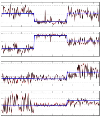
Figure 2 shows that the eigenvalues of L0 and Lˆ0, both in the main bulk and outside, are quite close to one another (precisely kL0 −Lˆ0k/kL0k ' 0.11). As for the eigenvectors (displayed in decreasing eigenvalue order), they are in an almost perfect match, as shown in Figure 3. In the latter is also shown in thick (blue) lines the theoretical approximated (signed) diagonal values of n1D(c−12)JTΠρJD(c−
1
2), which also show an extremely accurate match to the empirical class-wise means. Here, the k-means algorithm applied to the four displayed eigenvectors has a correct clustering rate of'86%. Introducing a −10dB random additive noise to the same MNIST data (see images in Figure 1) brings the approximation error down tokL0−Lˆ0k/kL0k '0.04and thek-means correct clustering probability to '78% (with only two theoretically exploitable eigenvectors instead of previously four).
0 10 20 30 40 50 0 0.5 1 1.5 2 ·10 −2 matching eigenvalues Eigenvalues ofL0 Eigenvalues ofLˆ0
Fig. 2. Eigenvalues ofL0andLˆ0, MNIST data,p= 784,n= 192.
V. CONCLUDING REMARKS
The random matrix analysis of kernel matrices constitutes a first step towards a precise understanding of the underlying
Fig. 3. Leading four eigenvectors ofL(red) versusLˆ(black) and theoretical class-wise means (blue); MNIST data.
mechanism of kernel spectral clustering. Our first theoretical findings allow one to already have a partial understanding of the leading kernel matrix eigenvectors on which clustering is based. Notably, we precisely identified the (asymptotic) linear combination of the class-basis canonical vectors around which the eigenvectors are centered. Currently on-going work aims at studying in addition the fluctuations of the eigenvectors around the identified means. With all these informations, it shall then be possible to precisely evaluate the performance of algorithms such ask-means on the studied datasets.
This innovative approach to spectral clustering analysis, we believe, will subsequently allow experimenters to get a clearer picture of the differences between the various classical spectral clustering algorithms (beyond the present Ng–Jordan–Weiss algorithm), and shall eventually allow for the development of finer and better performing techniques, in particular when dealing with high dimensional datasets.
REFERENCES
[1] U. Von Luxburg, “A tutorial on spectral clustering,” Statistics and computing, vol. 17, no. 4, pp. 395–416, 2007.
[2] A. Y. Ng, M. Jordan, and Y. Weiss, “On spectral clustering: Analysis and an algorithm,”Proceedings of Advances in Neural Information Processing Systems. Cambridge, MA: MIT Press, vol. 14, pp. 849–856, 2001. [3] N. El Karoui, “The spectrum of kernel random matrices,”The Annals of
Statistics, vol. 38, no. 1, pp. 1–50, 2010.
[4] F. Benaych-Georges and R. R. Nadakuditi, “The singular values and vectors of low rank perturbations of large rectangular random matrices,”
Journal of Multivariate Analysis, vol. 111, pp. 120–135, 2012. [5] F. Chapon, R. Couillet, W. Hachem, and X. Mestre, “The outliers among
the singular values of large rectangular random matrices with additive fixed rank deformation,”Markov Processes and Related Fields, vol. 20, pp. 183–228, 2014.