Novel Applications and Extensions for Bayesian Additive Regression Trees (BART) in Prediction, Imputation, and Causal Inference

(1)

Novel Applications and Extensions for Bayesian

Additive Regression Trees (BART) in Prediction,

Imputation, and Causal Inference

by

Yaoyuan Vincent Tan

A dissertation submitted in partial fulfillment of the requirements for the degree of

Doctor of Philosophy (Biostatistics)

in The University of Michigan 2018

Doctoral Committee:

(2)

Yaoyuan Vincent Tan

[email protected]

ORCID: 0000-0001-5950-9846

c

(3)

DEDICATION

To my Mom, Poh Wan Oh, who has been my emotional support throughout my MS and PhD studies as well as my aunt, Poh Kian Oh, for the same reasons.

(4)

ACKNOWLEDGEMENTS

This dissertation was written with extensive contributions and support from my thesis chair Dr. Michael R. Elliott as well as valuable comments from the members of my thesis committee Drs. Carol A.C. Flannagan, Jian Kang, Brisa S´anchez, and Kerby Shedden. Any mistakes or typographical errors are my own.

(5)

LIST OF FIGURES

Figure

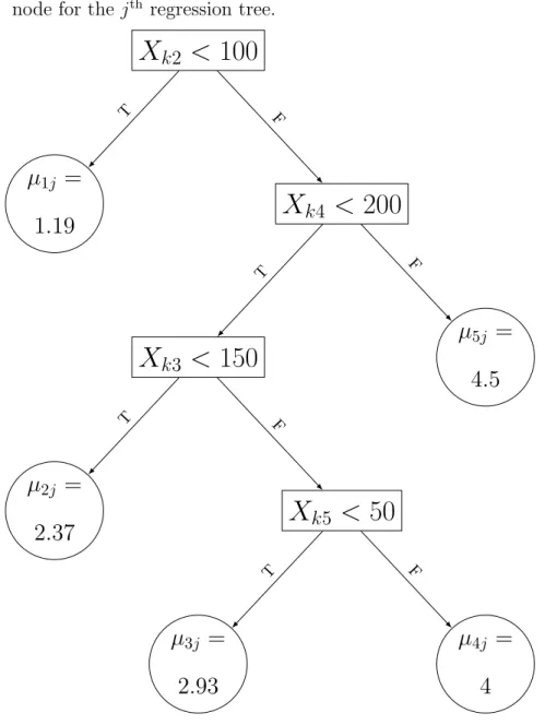
2.1 Example of a regression tree where µij is the mean parameter of the

ith _{node for the}_jth _{regression tree.} _{. . . .} ₈ 2.2 Regression tree, j = 1. . . 10 2.3 Regression tree, j = 2. . . 10 3.1 Boxplots of mean squared error (MSE) for continuous correlated

out-comes produced by BART, Fixed effects BART, and riBART. . . . 34 3.2 Boxplots of area under the receiver operating characteristic curve

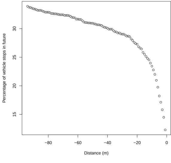
(AUC) for binary correlated outcomes produced by BART, Fixed effects BART, MLR, and riBART. . . 35 3.3 Proportion of vehicles in our study that would be stopped (≤1m/s)

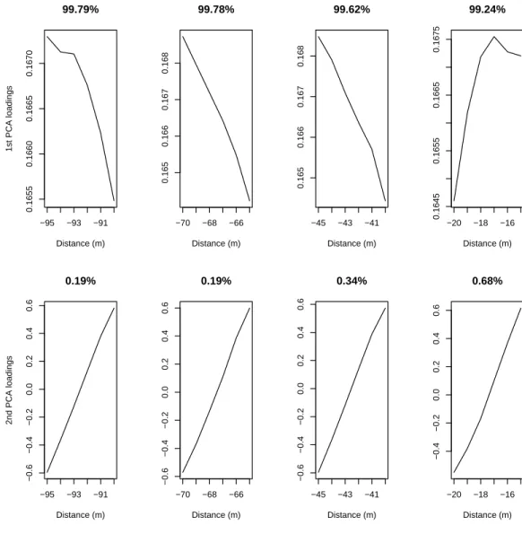
at some future point for each meter away from the center of an in-tersection. . . 40 3.4 Principal Component loadings for the first and second PC from

-95m to -90m, -70m to -65m, -45m to -40m, and -20m to -15m (left to right). The percentages indicate the proportion of variation explained by each PC. . . 42 3.5 Comparing the Area Under the receiver operating characteristic Curve

(AUC) profile gains of including each Principal Component (PC) in the logistic regression model. . . 43

(10)

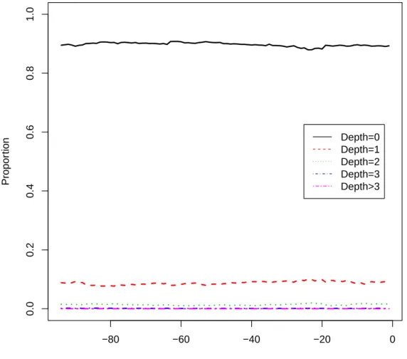
3.6 (a) The intra-class correlation (ICC) profile of riBART as a factor of distance from the intersection; (b) Area under the receiver operating characteristic curve (AUC) profile of riBART, BART, and random intercept logistic regression (dotted lines are 95% Credible Interval); and (c) AUC difference profile between riBART versus BART and riBART versus random intercept linear logistic regression. . . 47 3.7 Proportion of depth of regression tree meter by meter. . . 48 3.8 Smoothed (a) marginal effect of PC1 (b) marginal effect of PC2; and

(c) boxplots of the predicted probability of stopping stratified by the number of times a vehicle has stopped previously. Dotted red lines show smoothed 95% credible interval. . . 50

(11)

LIST OF TABLES

Table

2.1 Example data to explain sum of regression trees. . . 9 2.2 Posterior estimation for P2

j=1g(Xk, Tj,Mj) . . . 11

3.1 Simulation results for continuous correlated outcomes. Bias and cov-erage ofPm

j=1g(Xk, Tj,Mj)+ak(g(x)+ak) andσfor BART, riBART,

fixed effects BART, and multiple linear regression (MLR). . . 36 3.2 Simulation results for binary correlated outcomes. Bias and coverage

of Pm

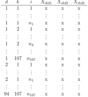
j=1g(Xk, Tj,Mj) + ak (g(x) + ak) for BART, riBART, fixed effects BART, and multiple linear logistic regression (MLLR). . . . 37 3.3 Example of resulting matrix for our IVBSS study dataset. . . 44 4.1 Bias, RMSE, 95% coverage, and average 95% confidence interval

length (AIL) of the eight estimators under the linear interaction in mean model scenario with sample size 1,000. . . 70 4.2 Bias, RMSE, 95% coverage, and average 95% confidence interval

length (AIL) of the eight estimators under the quadratic interaction in mean model scenario with sample size 1,000. . . 72 4.3 Bias, RMSE, 95% coverage, and average 95% confidence interval

length (AIL) under the Kang and Schafer (2007) example with sam-ple size 1,000. . . 73 4.4 Estimated population mean, and unadjusted odds ratios of injury

severity, any injury (ORNULL) or severe injury (ORSEV), where refer-ence group is delta-v less than 15 kph (X <15). . . 76

(12)

5.1 Sample example of a censoring by death dataset until t = 3 where

Zt= 1 indicates a subject having experienced a negative wealth shock

and Zt = 0 indicates a subject have not experienced any negative

wealth shock till time t . . . 94

5.2 Table of parameters for simulation . . . 103

5.3 Simulation results for sample size 4,000 . . . 106

5.4 Simulation results for sample size 8,000 . . . 107

5.5 Descriptive statistics of 1996 Health and Retirement Study (baseline), part 1 . . . 111

5.6 Descriptive statistics of 1996 Health and Retirement Study (baseline), part 2 . . . 112

5.7 Change in unadjusted cognitive score between consecutive waves strat-ified by negative wealth shock status . . . 112

5.8 Effect estimate of negative wealth shock on cognitive score for late middle aged adults in original Health Retirment Study cohort from 1996 to 2002. . . 115

F.1 Bias, RMSE, 95% coverage, and average 95% confidence interval length (AIL) of the eight estimators under the linear interaction in mean model scenario with sample size 500 using bootstrap. . . 144

F.2 Bias, RMSE, 95% coverage, and average 95% confidence interval length (AIL) of the eight estimators under the linear interaction in mean model scenario with sample size 1,000 using bootstrap. . . 145

F.3 Bias, RMSE, 95% coverage, and average 95% confidence interval length (AIL) of the eight estimators under the linear interaction in mean model scenario with sample size 5,000 using bootstrap. . . 146

F.4 Bias, RMSE, 95% coverage, and average 95% confidence interval length (AIL) of the eight estimators under the linear interaction in mean model scenario with sample size 500 using MI with posterior mean of propensity scores. . . 146

(13)

F.5 Bias, RMSE, 95% coverage, and average 95% confidence interval length (AIL) of the eight estimators under the linear interaction in mean model scenario with sample size 1,000 using MI with posterior mean of propensity scores. . . 147 F.6 Bias, RMSE, 95% coverage, and average 95% confidence interval

length (AIL) of the eight estimators under the linear interaction in mean model scenario with sample size 5,000 using MI with posterior mean of propensity scores. . . 147 F.7 Bias, RMSE, 95% coverage, and average 95% confidence interval

length (AIL) of the eight estimators under the linear interaction in mean model scenario with sample size 500 using MI with posterior draw of propensity scores. . . 148 F.8 Bias, RMSE, 95% coverage, and average 95% confidence interval

length (AIL) of the eight estimators under the linear interaction in mean model scenario with sample size 1,000 using MI with posterior draw of propensity scores. . . 148 F.9 Bias, RMSE, 95% coverage, and average 95% confidence interval

length (AIL) of the eight estimators under the linear interaction in mean model scenario with sample size 5,000 using MI with posterior draw of propensity scores. . . 149 F.10 Bias, RMSE, 95% coverage, and average 95% confidence interval

length (AIL) of the eight estimators under the quadratic interaction in mean model scenario with sample size 500 using bootstrap. . . . 150 F.11 Bias, RMSE, 95% coverage, and average 95% confidence interval

length (AIL) of the eight estimators under the quadratic interaction in mean model scenario with sample size 1,000 using bootstrap. . . 151 F.12 Bias, RMSE, 95% coverage, and average 95% confidence interval

length (AIL) of the eight estimators under the quadratic interaction in mean model scenario with sample size 5,000 using bootstrap. . . 152 F.13 Bias, RMSE, 95% coverage, and average 95% confidence interval

length (AIL) of the eight estimators under the quadratic interaction in mean model scenario with sample size 500 using MI with posterior mean of propensity scores. . . 152

(14)

F.14 Bias, RMSE, 95% coverage, and average 95% confidence interval length (AIL) of the eight estimators under the quadratic interac-tion in mean model scenario with sample size 1,000 using MI with posterior mean of propensity scores. . . 153 F.15 Bias, RMSE, 95% coverage, and average 95% confidence interval

length (AIL) of the eight estimators under the quadratic interac-tion in mean model scenario with sample size 5,000 using MI with posterior mean of propensity scores. . . 153 F.16 Bias, RMSE, 95% coverage, and average 95% confidence interval

length (AIL) of the eight estimators under the quadratic interaction in mean model scenario with sample size 500 using MI with posterior draw of propensity scores. . . 154 F.17 Bias, RMSE, 95% coverage, and average 95% confidence interval

length (AIL) of the eight estimators under the quadratic interac-tion in mean model scenario with sample size 1,000 using MI with posterior draw of propensity scores. . . 154 F.18 Bias, RMSE, 95% coverage, and average 95% confidence interval

length (AIL) of the eight estimators under the quadratic interac-tion in mean model scenario with sample size 5,000 using MI with posterior draw of propensity scores. . . 155 F.19 Bias, RMSE, 95% coverage, and average 95% confidence interval

length (AIL) under the Kang and Schafer (2007) example with sam-ple size 500 using bootstrap. . . 156 F.20 Bias, RMSE, 95% coverage, and average 95% confidence interval

length (AIL) under the Kang and Schafer (2007) example with sam-ple size 1,000 using bootstrap. . . 157 F.21 Bias, RMSE, 95% coverage, and average 95% confidence interval

length (AIL) under the Kang and Schafer (2007) example with sam-ple size 5,000 using bootstrap. . . 158 F.22 Bias, RMSE, 95% coverage, and average 95% confidence interval

length (AIL) under the Kang and Schafer (2007) example with sam-ple size 500 using MI with posterior mean of propensity scores. . . . 158 F.23 Bias, RMSE, 95% coverage, and average 95% confidence interval

length (AIL) under the Kang and Schafer (2007) example with sam-ple size 1,000 using MI with posterior mean of propensity scores. . . 159

(15)

F.24 Bias, RMSE, 95% coverage, and average 95% confidence interval length (AIL) under the Kang and Schafer (2007) example with sam-ple size 5,000 using MI with posterior mean of propensity scores. . . 159 F.25 Bias, RMSE, 95% coverage, and average 95% confidence interval

length (AIL) under the Kang and Schafer (2007) example with sam-ple size 500 using MI with posterior draw of propensity scores. . . . 160 F.26 Bias, RMSE, 95% coverage, and average 95% confidence interval

length (AIL) under the Kang and Schafer (2007) example with sam-ple size 1,000 using MI with posterior draw of propensity scores. . . 160 F.27 Bias, RMSE, 95% coverage, and average 95% confidence interval

length (AIL) under the Kang and Schafer (2007) example with sam-ple size 5,000 using MI with posterior draw of propensity scores. . . 161 G.1 Summary statistics stratified by missingness in total delta-v. . . 163 G.2 Summary statistics stratified by missingness in total delta-v, continued.164 G.3 Summary statistics stratified by missingness in total delta-v, continued.165 G.4 Summary statistics stratified by missingness in total delta-v, continued.166 G.5 Summary statistics stratified by missingness in total delta-v, continued.167 G.6 Summary statistics stratified by missingness in total delta-v, continued.168 G.7 Summary statistics stratified by missingness in blood alcohol

concen-tration (BAC) . . . 169 G.8 Summary statistics stratified by missingness in blood alcohol

concen-tration (BAC), continued . . . 170 G.9 Summary statistics stratified by missingness in blood alcohol

(16)

concen-LIST OF APPENDICES

Appendix

A. Derivations of the conditional draws and Metropolis-Hastings ratio in

BART . . . 125

B. Derivations of the conditional draws for riBART MCMC algorithm . . 130

C. Data preparation for Chapter III . . . 135

D. Consistency of the AIPWT estimator . . . 138

E. Consistency of the PSPP estimator . . . 140

F. Simulation Results for Sample Sizes 500, 1,000, and 5,000 . . . 143

G. Web Appendix D: Simple descriptive statistics for NASS-CDS 2014 and FARS 2015 . . . 162

(17)

ABSTRACT

The Bayesian additive regression trees (BART) is a method proposed by Chipman et al. (2010) that can handle non-linear main and multiple-way interaction effects for independent continuous or binary outcomes. It has enjoyed much success in areas like causal inference, economics, environmental sciences, and genomics. However, extensions of BART and application of these extensions are limited. This thesis discusses three novel applications and extensions for BART.

We first discuss how BART can be extended to clustered outcomes by adding a random intercept. This work was motivated by the need to accurately predict driver behavior using observable speed and location information with application to communication of key human-driver intention to nearby vehicles in traffic. Although our extension can be considered a special case of the spatial BART (Zhang et al., 2007), our approach differs by providing a relatively simple algorithm that allows application to clustered binary outcomes.

We next focus on the use of BART in missing data settings. Doubly robust (DR) methods allow consistent estimation of population means when either non-response propensity or modeling of the mean of the outcome is correctly specified. Kang and Schafer (2007) showed that DR methods produce biased and inefficient estimates when both propensity and mean models are misspecified. We consider the use of BART for modeling means and/or propensities to provide a “robust-squared” estimator that reduces bias and improves efficiency. We demonstrate this result, using simulations,

(18)

Zhang and Little, 2009). We successfully applied our proposed model to two national crash datasets to impute missing change in deceleration values (delta-v) and missing Blood Alcohol Concentration (BAC) levels respectively.

Our final effort considers how a negative wealth shock (sudden large decline in wealth) affects the cognitive outcome of late middle aged US adults using the Health Retirement Study, a longitudinal study of US adults, enrolled at age 50 and older and surveyed biennially since 1992. Our analysis faced three issues: lack of randomization, confounding by indication, and censoring of the cognitive outcome by a substantial number of deaths in our subjects. Marginal structural models (MSM), a commonly used method to deal with censoring by death, is arguably inappropriate because it upweights subjects who are more likely to die, creating a pseudo-population which resembles one where death is absent. We propose to compare the negative wealth shock effect only among subjects who survived under both sets of treatment regimens – a special case of principal stratification (Frangakis and Rubin, 2002). Because the counterfactual survival status would be unobserved, we imputed their survival status and restrict analysis to subjects who were observed and predicted to survive under both treatment regimes. We used a modified version of penalized spline of propensity methods in treatment comparisons (PENCOMP, Zhou et. al, 2018) to obtain a robust imputation of the counterfactual cognitive outcomes. Finally, we consider several possible extensions of these efforts for future work.

(19)

CHAPTER I

Introduction

Since its introduction in 2007 and formal publication in 2010, Bayesian additive regression trees (BART) has enjoyed much success in a variety of applications includ-ing biomarker discovery in proteomic studies (Hern´andez et al., 2015), estimating indoor radon concentrations (Kropat et al., 2015), estimation of causal effects (Leonti et al., 2010), genomic studies (Liu et al., 2010), hospital performance evaluation (Liu et al., 2015), prediction of credit risk (Zhang and H¨ardle, 2010), predicting power outages during hurricane events (Nateghi et al., 2011), prediction of trip durations in transportation (Chipman et al., 2010a), and somatic prediction in tumor experiments

(Ding et al., 2012). BART has also been extended to survival outcomes (Bonato

et al., 2011; Sparapani et al., 2016), multinomial outcomes (Kindo et al., 2016; Agar-wal et al., 2013), and heterogeneous outcomes (Green and Kern, 2012).

The primary reason for BARTs success is its ability to model non-linear main and multiple-way interaction effects without having to specify the type of non-linear or interaction mechanism. BART estimates multiple-way interactions ‘automatically’ by using regression trees which, in its simplest form (a constant mean parameter at the terminal nodes), can be viewed as an analysis of variance (ANOVA) model. To

(20)

improves. To keep BART from over-fitting, a strong prior is then placed on the tree structure of each regression tree to keep trees from growing too deep or too ‘bushy’ (trees with many terminal nodes).

Despite the flexibility, BART is still mostly applied to independent continuous or binary outcomes. Extensions and application of BART to situations outside of the independent continuous or binary outcomes setup are scarce. Two exceptions are

Zhang et al. (2007), who extended BART using a spatial random intercept to merge

two datasets in a statistical matched problem (R¨assler, 2002) and Low-Kam et al.

(2015), who modeled their terminal nodes of the regression tree as a cubic splines regression and used an autoregressive covariance matrix with truncated support on [0,1] to account for the correlation in their outcomes. These examples address com-plex extensions of BART to correlated continuous outcomes. Hence, in Chapter III of my thesis, I extended BART to correlated binary outcomes. For Chapter IV and V, I considered applications of BART to issues in the area of missing data and causal inference for longitudinal studies respectively.

I begin with a review chapter, where explicit details of how BART is formulated and implemented are discussed. Using a simple sum of two regression trees as an illustration, we will also attempt to answer a frequently asked question: “What is a sum of regression trees?” Included in this review chapter is also a brief discussion of why we think that application and extension of BART to models outside of the independent continuous and binary outcomes setting are lacking.

My next chapter was motivated by a project where the main aim was to deter-mine whether a human driven vehicle would stop at an intersection before executing a left-turn. To answer this question, we used data where drivers would drive cars fitted with devices to capture various vehicle dynamics like speed, acceleration, turn signal use, etc. We used the vehicle speed collected to construct a prediction model to determine whether a driver would stop at an intersection before executing a

(21)

left-turn. Preliminary work suggested that BART performed better and was more stable compared to many state-of-the-art machine learning methods, for example, Super Learner (van der Laan and Polley, 2010). Unfortunately, BART was designed for independent outcomes but in our data, each driver could take multiple left turns cre-ating correlation among our binary outcomes. Thus far, there has been no literature extending BART to handle correlated binary outcomes. Hence, we introduced a ran-dom intercept to BART to handle clustered binary outcomes. The crucial idea lies in the fact that given a draw of the random intercept, the resulting model is once again BART and the BART algorithm can be applied to estimate the remaining parameters. We found that our proposed method, which we call “random intercept BART (riB-ART)”, produced better empirical prediction properties compared to BART without the random intercept in simulations with correlated continuous or binary outcomes and when applied to our data.

Chapter IV focuses on the area of missing data. Under the missing at random (MAR) assumption, doubly robust (DR) estimators provide a consistent estimate of the mean when either the mean or propensity model is correctly specified. Unfortu-nately,Kang and Schafer (2007) showed using a simulation example that DR estima-tors could be highly biased and inefficient when both the propensity and mean model are modestly misspecified. We recognized that the misspecification of the propensity and mean model in Kang and Schafer’s example mainly comes from the fact that common regression methods have difficulty in specifying a model that can handle non-linear main and multiple-way interaction effects. Hence, we propose to replace the usual regression models in DR estimators with BART and investigate whether such a strategy would improve the bias and efficiency of common DR estimators. We found that by replacing the model specification of the various DR estimators with

(22)

paring our proposed estimator with existing DR estimators, we could get a sense of the relationship of the outcome of interest with the various covariates in the data.

In Chapter V we turn our attention to a causal inference problem in the context of longitudinal studies. This work was motivated by the Health and Retirement Survey (Sonnega et al., 2014) which is a longitudinal study of US adults, enrolled at age 50 and older. Enrolled subjects were surveyed biennially starting from 1992 with detailed modules on financial status and health. The primary aim of this work was to determine how the cognitive ability of late middle aged US adults is affected by a negative wealth shock, i.e. a sudden large decline in wealth. We faced three issues in this analysis. First, there is a lack of randomization for which subjects get a negative wealth shock; factors like socio-economic status and gender are likely confounders. Second, the risk of receiving a negative wealth shock may depend on prior cognitive ability, a situation commonly termed as “confounding by indication”. Finally, and most importantly, death occurs at a 13% higher rate during follow-up in our data, causing a large proportion of our outcomes to be censored. A common approach is to employ Marginal Structural Models (MSM, Robins et al., 2000) which accounts for confounding by indication and censoring by death by weighting using the inverse probability of the treatment received based on the previous values of the time-varying covariates and outcomes and inverse probability of death respectively. The issue with this approach – perhaps much under appreciated – is that by weighting using the inverse probability of death, subjects who are more likely to die would be upweighted creating a pseudo-population which resembles one where death is absent over time (Chaix et al., 2012). We propose to compare the effect of a negative wealth shock on cognitive outcome only among subjects who would potentially survive under both sets of treatment regimes, a special case of principal stratification (Frangakis and Rubin, 2002). Because the survival status of the counterfactuals (for example, negative wealth shock survival status of subjects who did not get a negative wealth shock and

(23)

vice versa) are unobserved, we imputed their survival status and restricted analysis to subjects who were observed and predicted to have survived. We then modified the penalized spline of propensity methods in treatment comparisons (PENCOMP,

Zhou et al., 2018) using BART to impute the counterfactual cognitive ability among this restricted set. This modified version of PENCOMP is doubly robust and eases the model specification burden on the researcher. Simulation studies suggested that our proposed method worked better than existing methods. Results from our data analysis also suggested a slightly different estimate of the effect of a negative wealth shock on cognitive ability compared to MSM.

(24)

CHAPTER II

Review

2.1 Bayesian additive regression trees

We next review in detail the Bayesian additive regression trees (BART) model pro-posed by Chipman et al. (2010b) for independent continuous and binary outcomes. Included in this review is a discussion of what a regression tree is and what a “sum of regression trees” mean. We also discuss how the prior distribution and hyperpa-rameters are set as well as how the posterior distribution of BART is calculated.

2.2 Setup

Suppose we have n subjects indexed by k and we have outcomes Yk. For

contin-uous outcomes, Yk ∈ R, while for binary outcomes, Yk ∈ {0,1}. In addition to the

outcomes, we have p predictors/covariates notated as Xk = (Xk1, . . . , Xkp)T. The

objective of BART is to estimate a flexible model to fit the following problem

Yk=f(Xk) +k (2.1)

where k i.i.d

(25)

2.3 Continuous outcomes

2.3.1 Model and regression trees

For continuous outcomes, BART estimates equation (2.1) as

Yk= m X j=1 g(Xk, Tj,Mj) +k k i.i.d. ∼ N(0, σ2) (2.2)

where Tj is the jth binary tree structure and Mj = (µ1j, . . . , µbjj)T is the set of bj

terminal node parameters associated with tree structureTj. Typically, the number of

trees m is fixed and no prior distribution is placed on m. Chipman et. al. suggested fixingmat 200 as this performs well in many situations. Alternatively, they suggested using cross-validation to determine m.

The binary tree Tj is made up of both internal nodes and terminal nodes. At

each internal node, there is a decision rule that splits estimation of the mean of Yk

depending on the covariatesXk. For example in Figure 2.1, the first internal node at

the top of the tree drops the mean to the left if the corresponding covariateXk2 <100 or to the right ifXk2 ≥100. At a terminal node (a node with no decision rules to split an outcome), the sample mean of the outcomes allocated to the terminal node can be calculated to obtain the parameter µij at the terminal node. Thus, g(Xk, Tj,Mj)

can be viewed as thejth _{function that assigns the mean} _µ

(26)

Figure 2.1: Example of a regression tree where µij is the mean parameter of the ith

node for thejth _{regression tree.}

X

k2

<

100

µ

1j

=

1 .

19

T

X

k4

<

200 X

k3

<

150

µ

2j

=

2 .

37

T

X

k5

<

50

µ

3j

=

2 .

93

T

µ

4j

=

4

F F T

µ

5j

=

4 .

5

F F

(27)

can be similarly expressed as

Yk=µ1jI{Xk2 <100}+µ2jI{Xk2 ≥100}I{Xk4 <200}I{Xk3 <150} +µ3jI{Xk2 ≥100}I{Xk4 <200}I{Xk3 ≥150}I{Xk5 <50} +µ4jI{Xk2 ≥100}I{Xk4 <200}I{Xk3 ≥150}I{Xk5 ≥50} +µ5jI{Xk2 ≥100}I{Xk4 ≥200}+k

where I{.} is the indicator function and k i.i.d.

∼ N(0, σ2). This representation as an ANOVA model clearly shows how a regression tree handles multiple-way interactions. In equation (2.2), note that we have a sum ofg(Xk, Tj,Mj) or, a sum of regression

trees. What is a sum of regression trees? We attempt to explain this using a simplified example. Supposep= 3, n = 10, and we have the following data.

Table 2.1: Example data to explain sum of regression trees.

k Y X1 X2 X3 1 Y1 -182 235 -333 2 Y2 54 339 244 3 Y3 -106 -50 -682 4 Y4 -80 -62 -320 5 Y5 -123 198 -77 6 Y6 175 108 -46 7 Y7 -44 11 136 8 Y8 -131 -10 -70 9 Y9 -56 68 257 10 Y10 7 324 282

(28)

Carlo Markov Chain (MCMC) draws (See Figures 2.2 and 2.3).

Figure 2.2: Regression tree, j = 1.

X

k1

<

100 X

k2

<

200

ˆ

µ

11 T

ˆ

µ

21 F T

ˆ

µ

31 F

Figure 2.3: Regression tree, j = 2.

X

k3

<

100

ˆ

µ

12 T

X

k2

<

200

ˆ

µ

22 T

ˆ

µ

32 F F

For this hypothetical example, the resulting posterior estimation ofP2

j=1g(Xk, Tj,Mj)

(29)

Table 2.2: Posterior estimation for P2 j=1g(Xk, Tj,Mj) k Y g(X, T1,M1) g(X, T2,M2) P2 j=1g(X, Tj,Mj) 1 Y1 µˆ21 µˆ12 µˆ21+ ˆµ12 2 Y2 µˆ21 µˆ22 µˆ21+ ˆµ22 3 Y3 µˆ11 µˆ12 µˆ11+ ˆµ12 4 Y4 µˆ11 µˆ12 µˆ11+ ˆµ12 5 Y5 µˆ11 µˆ12 µˆ11+ ˆµ12 6 Y6 µˆ31 µˆ12 µˆ31+ ˆµ12 7 Y7 µˆ11 µˆ22 µˆ11+ ˆµ22 8 Y8 µˆ11 µˆ12 µˆ11+ ˆµ12 9 Y9 µˆ11 µˆ22 µˆ11+ ˆµ22 10 Y10 µˆ21 µˆ32 µˆ21+ ˆµ32

where ˆµij ∼h(Rk1j+Rk2j+. . .+Rk_ni,j, θ), withh(.) being the posterior distribution ofµij,θbeing the set of prior hyperparameters forµij,Rkj =Yk−P_l6=jg(Xk, Tl,Ml)

being the residual data taken in by h(.) to obtain the posterior distribution of µij,

and ni being the number of residuals Rkj allocated to the terminal node µij by the

jth _{regression tree. For example, ˆ}_µ

21 ∼ h(R11+R21+R10,1, θ) with R11 =Y1−µˆ12,

R21 =Y2−µˆ22, andR10,1 =Y10−µˆ32; ˆµ12∼h(R12+R32+R42+R52+R62+R82, θ), with

R12 =Y1−µˆ21,R32=Y3−µˆ11,R42 =Y4−µˆ11,R62=Y6−µˆ31, andR82 =Y8−µˆ11; etc. Note that during the posterior estimation of g(Xk, Tj,Mj) for each j, the residuals

Rk1j, Rk2j, . . . , Rk_ni,j are used instead of Yk1, . . . , Yk_ni. Hence, we estimate Yk using the sum of the allocated parameters ˆµij instead of their mean. To obtain ˆµij, an

(30)

this ‘additive’ property of BART allows estimation of non-linear effects easily without having a need to specify the form of non-linear relationship between the outcomes and predictors.

2.3.2 Prior distribution

In subsection 2.3.1, we assumed that the tree structure was specified. Of course, we would like the data to determine the tree structure. BART does this in a Bayesian framework, first specifying a prior on the tree structure, terminal node parameters, and variance. The joint prior distribution for (2.2) is

P[(T1,M1), . . . ,(Tm,Mm), σ]. (2.3)

Assuming independence of k and (Tj,Mj) and between all m tree structures and

terminal node parameters, equation (2.3) can be decomposed as

P[(T1,M1), . . . ,(Tm,Mm), σ] = [ m Y j=1 P(Tj,Mj)]P(σ) = [ m Y j=1 P(Mj|Tj)P(Tj)]P(σ) = [ m Y j=1 { bj Y i=1 P(µij|Tj)}P(Tj)]P(σ).

where i= 1, . . . , bj indexes the terminal node parameters in tree j. The prior

distri-bution of µij|Tj and σ2 can be specified as

µij|Tj ∼N(µµ, σµ2),

σ2 ∼IG(ν 2,

νλ

(31)

where IG(α, β) is the inverse gamma distribution with shape parameter α and rate parameterβ. The prior forP(Tj) can be specified using three aspects. The first is the

probability that a node at depthd= 0,1,2, . . .is an internal node, which isα(1+d)−β

where α ∈ (0,1) and β ∈ [0,∞). Here, α controls how likely a terminal node in the tree would split, with smaller α implying a lesser likelihood that a terminal node would split, and β controls the number of terminal nodes with a larger β decreasing the number of terminal nodes. The second aspect is the distribution used to choose which covariate is selected for the decision rule in an internal node. The final aspect is the distribution for the value of the selected covariate for the decision rule in an internal node. For the distribution in the second and third aspect ofP(Tj), the default

distirbution used is the discrete uniform distribution for the available covariates. A more flexible distribution like the multinomial distribution with certain variables or values weighted higher can be used (Kapelner and Bleich, 2016).

2.3.3 Hyperparameters

The specification of these priors implies that the following hyperparameters need to be set: α, β, µµ, σµ, ν, and λ. These hyperparameters are constructed as a mix

of apriori fixed and data-driven. For α and β, the default values of α = 0.95 and

β = 2 provide a balanced penalizing effect for the probability of a node splitting. For

µµ and σµ, they are set such that E[Yk|Xk]∼N(mµµ, mσµ2) assigns high probability

to the interval (min

k (Yk),maxk (Yk)). This can be achieved by defining v such that

min k (Yk) = mµµ −v √ mσµ and max k (Yk) = mµµ +v √

mσµ. For ease of posterior

distribution calculation, Yk is transformed by ˜Yk = Yk− min k (Yk)+maxk (Yk) 2 max k (Yk)−mink (Yk) . This results in ˜ Yk ∈ (−0.5,0.5) where min

k (Yk) = −0.5 and maxk (Yk) = 0.5. This has the effect of

(32)

default value for ν is 3 and λ is the value such that P(σ2 _{< s}2_;_{ν, λ}_{) = 0}_._{9 where} _s2 is the estimated variance of the residuals from the multiple linear regression with Yk

as the outcomes and Xk as the covariates.

2.3.4 Posterior distribution calculation

The prior distribution and hyperparameters would induce the posterior distribu-tion P[(T1,M1), . . . ,(Tm,Mm), σ|Yk]∝P(Yk|(T1,M1), . . . ,(Tm,Mm), σ) ×P((T1,M1), . . . ,(Tm,Mm), σ) where P(Yk|(T1,M1), . . . ,(Tm,Mm), σ) ∼ N( Pm j=1g(Xk, Tj,Mj), σ2) which can be

simplified to two major posterior draws using Gibbs sampling. First, drawm succes-sive

P[(Tj,Mj)|T(j),M(j), Yk, σ] (2.4)

for j = 1, . . . , m, where T(j) and M(j) consist of all the tree structures and terminal nodes except for the jth _{tree structure and terminal node; then, draw}

P[σ|(T1,M1), . . . ,(Tm,Mm), Yk] (2.5)

fromIG(ν+₂n,νλ+

Pn

k=1(yk−Pmj=1gk(Xk,Tj,Mj))2

2 ).

To obtain a draw from (2.4), note that this distribution depends on (T(j),M(j), Yk, σ)

through

Rkj =Yk−

X

w6=j

g(Xk, Tw,Mw), (2.6)

the residuals of them−1 regression sum of trees fit excluding thejthtree. Thus (2.4) is equivalent to the posterior draw from a single regression treeRkj =g(Xk, Tj,Mj) +k

(33)

or

P[(Tj,Mj)|Rj, σ]. (2.7)

We can obtain a draw from (2.7) by first integrating out Mj to obtain P(Tj|Rj, σ).

This is possible since a conjugate prior on µij was employed. We draw P(Tj|Rj, σ)

using a Metropolis-Hastings (MH) algorithm where first, we generate a candidate tree

T_j∗ for thejth _{tree with probability distribution}_q₍_T

j, Tj∗) and then, we acceptTj∗ with

probability α(Tj, Tj∗) = min{1, q(T_j∗, Tj) q(Tj, Tj∗) P(Rj|X, T_j∗, Mj) P(Rj|X, Tj, Mj) P(T_j∗) P(Tj) }. (2.8)

A new treeT_j∗ can be proposed given the previous treeTj by four steps: (i) grow,

where a terminal node is split into two new child nodes; (ii) prune, two terminal child nodes immediately under the same non-terminal node are combined together such that their parent non-terminal node becomes a terminal node; (iii) swap, the splitting criteria of two non-terminal nodes are swapped; (iv) change, the splitting criteria of a single non-terminal node is changed. Once we drawP(Tj|Rj, σ), we then

draw P(µij|Tj,Rj, σ) ∼ N( σ2 µ Pni i rij niσ2 µ+σ2 , σ2_σ2 µ niσ2

µ+σ2), where rij is the subset of elements in Rj allocated to the terminal node parameterµij andni is the number ofrijs allocated

toµij.

Complete details for the derivation of P(µij|Tj,Rj, σ), equation (2.5) as well as

the explicit formula for equation (2.8) for the grow and prune steps can be found in Appendix A.

(34)

where Φ[.] is the cumulative distribution function of a standard normal distribution and G(Xk) = m X j=1 g(Xk, Tj,Mj). (2.10)

The notation m, Tj, and Mj are similar to equation (2.2) and m by default is once

again set at 200.

Because we employed a probit link, we may view the binary outcomes BART as the continuous outcomes BART withσ≡1. Hence, only prior distributions forTj and

µij|Tjneed to be specified under binary outcomes BART. The same prior distributions

as continuous outcomes BART can be used. The α and β hyperparameters are the same but the µµ and σµ hyperparameters are specified differently from continuous

outcomes BART. To set the hyperparameters for µµ andσµ, Chipman et al. suggests

µµ = 0 and σµ = _v√3_m where v = 2 would result in an approximate 95% probability

that draws ofG(Xk) will be within (−3,3).

To draw the posterior distribution of Tj and µij, we first use data augmentation

(Tanner and Wong, 1987;Albert and Chib, 1993) to draw a continuous latent variable

Zk givenYk. Chipman et al. (2010b) suggests drawing Zk as

Zk=      max(N(G(Xk),1),0) if Yk = 1 min(N(G(Xk),1),0) if Yk= 0. (2.11)

We differ slightly by drawingZk as

Zk =      N(0,∞)(G(Xk),1) if Yk = 1 N(−∞,0)(G(Xk),1) if Yk= 0. (2.12)

where N(a,b)(µ, σ2) is the normal distribution with mean µ variance σ2 truncated to (a, b). We then replace the continuous outcomes Yk in equations (2.4) to (2.8) with

(35)

can be updated followed by Zk. The algorithm then iterates between the draws of

Zk,Tjs, and µijs until convergence.

2.5 Motivation for re-writing BART code and future work

In summary, the BART algorithm for continuous and binary outcomes can be visualized as follows:

INPUT: Yk outcome andXk covariates. OUTPUT:Pm

j=1ˆg(Xk, Tj,Mj) and ˆσfor continuous outcomes, ˆG(Xk) for binary outcomes.

BART algorithm(Yk,Xk){

1. If outcome is continuous, transformYk to the range (−0.5,0.5). If outcome

is binary, draw Zk.

2. Setup hyperparametersα, β, σµ, and for continuous outcomes ν and λ.

3. Draw (Tj, Mj)|T(j),M(j), Yk, σ for j = 1, . . . , m.

• Draw P[Tj|T(j),M(j), Yk, σ] using Metropolis-Hastings algorithm. – Propose a new tree using either grow, prune, change, or swap.

– Accept a new tree based on equation (2.8).

• Draw P[Mj|Tj, T(j),M(j), Yk, σ].

4. If outcome is continuous, drawP[σ|(T1,M1), . . . ,(Tm,Mm), Yk]. If outcome

is binary, σ is fixed at 1.

(36)

Based on the above algorithm, there are four publicly available software packages that can implement the BART algorithm. They are

• BayesTree from Chipman et al. (2010b),

• bartMachine from Kapelner and Bleich (2016),

• Parallel BART from Pratola et al. (2014), and

• dbarts fromChipman et al. (2015).

The first three packages implement BART as a whole complete function i.e., there are no separate functions for 1-4. dbarts allows a single MCMC draw of 3 and 4. It is immediately clear that these implementations of BART are not modular in the sense that it is not easy to manipulate or modify any of the steps and substeps in the algorithm, especially for step 3. Due to this lack of modularity, extensions of BART to other outcomes or applying BART into other research areas would be tedious since the researcher will have to re-write the BART algorithm from scratch when often, an extension will only require a slight modification of one step or substep within the BART algorithm.

In order to provide the researcher flexibility in the implementation of BART, we re-coded the BART algorithm inR such that each substep in 3 is a separate function and step 4 is a separate function on its own. For step 3, this means that we have a separate function which can propose a new tree structure and another function which can accept or reject a new tree structure. Once the tree structure is fixed, we then have another function to draw the terminal nodes in the tree structure. Such flexibility can allow researchers to extend BART easily or modify different parts of the BART model to suit their own research application. In addition, by providing the codes in R, our implementation allows the researcher to easily follow the BART algorithm. To maintain efficiency, we then used Rcpp to re-write ourR codes.

(37)

2.6 Discussion

In this chapter, we reviewed BART in great detail re-coded the BART algorithm to help us better understand the mechanism of BART. Our codes allows them drawn tree structures at each MCMC to be extracted, hence, enchancing the interpretabil-ity of BART compared to existing methods. In terms of prediction performance compared to other existing machine learning methods like Lasso, Gradient boost-ing, Neural nets, and Random forests, Chipman et al. (2010b) already showed that BART was either comparable or performed better. Literature regarding the compu-tation complexity of BART compared to these machine learning methods is a topic for future investigation.

(38)

CHAPTER III

Predicting human-driving behavior to help

driverless vehicles drive: random intercept

Bayesian Additive Regression Trees

3.1 Introduction

In transportation statistics, a new area of research brought about by improve-ments in artificial intelligence and engineering is the creation of the autonomous (self-driving) vehicle. These vehicles have been tested on city streets in certain lo-cations since 2009. A number of companies have deployed or announced plans for deployment of such vehicles (Google, 2015; Mchugh, M., 2015; Davies, A., 2015). A major hurdle for self-driving vehicles on public roads is that these vehicles will have to interact with human-driven vehicles for the foreseeable future. Human drivers do not always communicate their plans to other drivers well. For example, when making a turn, the turn signal is the only explicit means of communicating plans, and even they are used with less than perfect reliability. Hence, the ability to deploy driverless vehicles on a large scale will critically depend on the development of a good prediction model for human driving behavior.

Currently, driverless vehicles developed generally use onboard sensors to gather data from their surrounding environment to make driving decisions. We envision in

(39)

the future that vehicles (both human driven and driverless) would be connected such that a driving intent model could first be evaluated on the human driver’s vehicle and subsequently “communicated” to the driverless vehicle enabling it to make a better driving decision. Such vehicle-to-vehicle communication would become increasingly available as technology improves resulting in a connected environment. Under such a connected environment, developing a good prediction model for human driving behavior would make sense especially when the driving pattern of a human driven vehicle depends heavily on the unique tendencies of the human driver.

Building a prediction model that addresses all or most of the human driving be-havior and driving intent is a massive and complex task. To keep this paper concise, we focus on the the development of a prediction model for a single driving behavior: whether a human driver would stop at an intersection before executing a left turn. We are particularly interested in left turn stops because in countries with right-side driving, for example, US, left turn crashes can result in severe passenger-side impacts. Since left turn maneuvers already present a challenge for human drivers, we expect this maneuver to present difficulty for the driverless vehicle. Placing this prediction scenario in the context of a connected environment, the driverless vehicle will be evaluating data from the human-driven vehicle, supplied from an adapted version of existing “black-box” technology that would broadcast speed and location informa-tion to driverless vehicles. The connected driverless vehicle would then combine this transmitted information together with the data it has gathered from its surrounding environment to make a driving decision.

To develop such a prediction model, we used a naturalistic driving study, the Inte-grated Vehicle Based Safety System (IVBSS) study Sayer et al. (2011). Naturalistic driving studies (including the IVBSS) involve the collection of driving data from

(40)

ve-Typical data collected include vehicle speed, brake application, and miles traveled. Prediction models in statistics typically rely on regression models that require estimation of covariate main effects and interactions, and, when predictors are con-tinuous or on a fine ordinal scale, assessment of non-linearities. In the settings where understanding associations or, under appropriate assumptions, causal mechanism be-tween predictors and outcomes are of interest, approximations for non-linearities and averaging over interactions might be used to develop summaries to ease interpreta-tion. In prediction, since obtaining the most accurate forecast is the goal, estimating highly complex non-linearities, including the interactions, is at a premium, as long as these non-linearities are true signals and not noise.

Perhaps the most common method for modeling non-linearity is to use a poly-nomial transformation for a covariate, usually centered at the mean to reduce corre-lation. More sophisticated approaches use penalized splines or additive models that only require assumptions of smoothness (existence of derivatives) to obtain consistent estimates of a non-linear trend Hastie and Tibshirani (1990); Ruppert et al. (2003). Modeling of non-linear interactions between two or more predictors using thin-plate splinesFranke (1982) can quickly become difficult, suffering from the “curse of dimen-sionality”, as the data required to estimate high-dimensional surfaces become enor-mous. In the binary outcomes setting, methods such as classification and regression trees (CART; Breiman et al., 1984) as well as more sophisticated machine learning techniques such as artificial neural networks (ANN; Smith et al., 1993) and support vector machines (SVM; Gammermann, 2000) are commonly used. Although CART is able to model complex interactions naturally, it faces difficulty when modeling non-linear interactions. In contrast, ANN and SVM excel at modeling non-non-linearities but may face difficulties when modeling complex interactions.

Because our goal is prediction, we prefer regression methods that are able to account for non-linear main and multiple-way interaction effects. Bayesian additive

(41)

regression trees (BART;Chipman et al., 2010b) is one such model which allows flexible estiamtion of non-linear main and multiple-way interaction effects without much input from the researcher. Hence, we employed BART to predict whether a human-driven vehicle would stop before executing a left turn at an intersection. However, BART was designed for independent subjects, but we would like to evaluate the tendencies of each driver and decide whether including their tendency would improve the prediction of whether a human-driven vehicle would stop before executing a left turn. We are aware of two papers that extended BART to handle longitudinal or clustered observations:

Zhang et al. (2007) used a spatial random intercept BART to merge two datasets,

and Low-Kam et al. (2015) did so in a dose-finding toxicity study. Zhang et al.

(2007) developed an imputation model for a statistical matching problem R¨assler

(2002) that used BART with a conditional auto-regressive distribution for the random intercept. Since the correlation our dataset was induced by repeated measurements and not spatial effects, the distribution Zhang et al. (2007) placed on the random intercept may not be appropriate. Moreover, they did not discuss how their model could be extended to clustered binary outcomes. Low-Kam et al.(2015) investigated the associations between the physico-chemical properties of nanoparticles and their toxicity profiles over multiple doses. The complex nature of their goal prompted them to first specify an autoregressive covariance matrix with truncated support on [0,1] to handle the correlated measurements, and then they specified a conditionally conjugate P-spline prior for the terminal nodes of the regression trees. The complexity of their method makes implementation to our dataset difficult since our outcomes are binary. Neither papers provided convenient software for implementing their methods.

Motivated by the lack of an appropriate and straightforward method to implement BART to handle clustered binary outcomes, we propose an extension of BART to

(42)

BART (riBART). We proceed by first providing a review of BART in the next section followed by a discussion of how we extended BART to riBART in Section 3. In Section 4, we use a simulation study to compare the performance of riBART against BART, fixed effects BART, and linear regression models when applied to clustered datasets. We implement riBART on our dataset and compare its prediction performance with BART, fixed effects BART, random intercept linear logistic regression, and multiple linear logistic regression in Section 5. Finally, we conclude with a discussion and possible future work in Section 6.

3.2 Bayesian Additive Regression Trees

3.2.1 Continuous outcomes

Denote a continuous outcomeYkwith associatedpcovariatesXk = (Xk1, . . . , Xkp)T

for k = 1, . . . , n subjects. BART models the outcome as

Yk= m X j=1 g(Xk, Tj,Mj) +k k i.i.d. ∼ N(0, σ2) (3.1)

where Tj is the jth binary tree structure and Mj = (µ1j, . . . , µbjj)T is the set of bj

terminal node parameters associated with tree structure Tj Chipman et al. (2010b).

g(Xk, Tj,Mj) can be viewed as the jth function that assigns the mean µij to the kth

outcome, Yk. Typically, the number of trees m is fixed and no prior distribution is

placed on m. Chipman et al. (2010b) suggested setting m = 200 as this performs well in many situations. Alternatively, cross-validation could be used to determine m

Chipman et al. (2010b).

The joint prior distribution for Eq. (3.1) is P[(T1,M1), . . . ,(Tm,Mm), σ]. Note

that by the independence of k and (Tj,Mj) as well as the independence between

(43)

P[(T1,M1), . . . ,(Tm,Mm), σ] can be decomposed as P[(T1,M1), . . . ,(Tm,Mm), σ] = [ m Y j=1 P(Tj,Mj)]P(σ) = [ m Y j=1 P(Mj|Tj)P(Tj)]P(σ) = [ m Y j=1 { bj Y i=1 P(µij|Tj)}P(Tj)] ×P(σ).

where i = 1, . . . , bj indexes the terminal node parameters in tree j. This implies

that we need to assign priors to Tj, µij|Tj, and σ in order to obtain the posterior

distributions of Tj, µij, and σ. Chipman et al. (2010b) suggested the following prior

distributions on µij|Tj and σ: µij|Tj ∼N(µµ, σµ2), σ2 ∼IG(ν 2, νλ 2 ).

where IG(α, β) is the inverse gamma distribution with shape parameter α and rate parameter β. The prior distribution of P(Tj) can be specified using three aspects:

(i) the probability that a node at depth d = 0,1,2, . . . is an internal node given by α(1 + d)−β where α ∈ (0,1) and β ∈ [0,∞) so that α controls how likely a terminal node in the tree would split, with a smaller α implying lesser likelihood a terminal node would split, and β controls the number of terminal nodes, and a largerβ decreasing the number of terminal nodes; (ii) the distribution used to choose which covariate to be selected for the decision rule in an internal node; and (iii) the distribution for the value of the selected covariate for the decision rule in an internal

(44)

distributions could be usedKapelner and Bleich (2016).

In Chipman et al. (2010b), α = 0.95 andβ = 2. For µµ and σµ, they are set such

that N(mµµ, mσ2µ) assigns high probability to the interval (min

k (Yk),maxk (Yk)). This

can be achieved by defining v such that min

k (Yk) = mµµ−v √ mσµ and max k (Yk) = mµµ+v √

mσµ. For convenience when implementing the posterior draws ofTj andµij,

Chipman et al.(2010b) suggested transforming the observedYkto ˜Yk = Yk− min k (Yk)+maxk (Yk) 2 max k (Yk)−mink (Yk) , and then treating ˜Yk as the outcome. This has the effect of allowing the

hyperpa-rameter of µµ to be set as µµ = 0 and σµ to be set as σµ = _v0√.5_m where v is to be

chosen. For v = 2, N(mµµ, mσ2µ) assigns a prior probability of 0.95 to the interval

(min

k (Y),maxk (Y)) and is the suggested value. Finally for ν and λ, Chipman et al.

(2010b) suggested setting ν = 3 and λ is the value such that P(σ2 _{< s}2_;_{ν, λ}_{) = 0}_.₉ wheres2 _{is the estimated variance of the residuals from the multiple linear regression} with Yk as the outcomes and Xk as the covariates.

This setup induces the posterior distributionP[(T1,M1), . . . ,(Tm,Mm), σ|Yk] which

can be simplified to two major posterior draws using Gibbs sampling. First, draw m

successive

P[(Tj,Mj)|T(j),M(j), Yk, σ] (3.2)

for j = 1, . . . , m, where T(j) and M(j) consist of all the tree structures and ter-minal nodes except for the jth _{tree structure and terminal node; and then, draw}

P[σ|(T1,M1), . . . ,(Tm,Mm), Yk].

To obtain a draw from Eq. (3.2), note that this distribution depends on (T(j),M(j), Yk, σ) through

Rkj =Yk−

X

w6=j

g(Xk, Tw,Mw), (3.3)

the residuals of the m−1 regression sum of trees fit excluding the jth _{tree. Thus,} Eq. (3.2) is equivalent to the posterior draw from a single regression tree Rkj =

(45)

g(Xk, Tj,Mj) +k or

P[(Tj,Mj)|Rkj, σ]. (3.4)

We can obtain a draw from Eq. (3.4) by first drawing from P(Tj|Rkj, σ) using a

Metropolis-Hastings (MH) algorithm outlined in Chipman et al. (1998). A new tree

T_j∗can be proposed given the previous treeTj by four steps: (i) grow, where a terminal

node is split into two new child nodes; (ii) prune, where two terminal child nodes immediately under the same non-terminal node is combined together such that their parent non-terminal node becomes a terminal node; (iii) swap, where the splitting criteria of two non-terminal nodes are swapped; (iv) change, where the splitting criteria of a single non-terminal node is changed. Once we drawP(Tj|Rkj, σ), we then

drawP(µij|Tj, Rkj, σ)∼N( σ2 µ Pni i rij+σ2µµ niσ2 µ+σ2 , σ2_σ2 µ niσ2

µ+σ2), whererij is the subset of elements

inRkj allocated to the terminal node with parameterµij and ni is the number ofrijs

in Rkj allocated to µij. Note that µµ = 0 after transformation. Complete details for

the derivation of P(µij|Tj, Rkj, σ) and P[σ|(T1,M1), . . . ,(Tm,Mm), Yk] are provided

in the supplementary materials available online. Explicit MH algorithm details for Eq. (3.4) can be found in Appendix A of Kapelner and Bleich (2016).

3.2.2 Binary outcomes

Extending BART to binary outcomes involve a modification of Eq. (3.1). First, let G(Xk) = m X j=1 g(Xk, Tj,Mj). (3.5)

Using the probit formulation, the binary outcomesYkcan be linked to Eq. (3.5) using

P(Yk= 1|Xk) = Φ[G(Xk)] where Φ[.] is the cumulative density function of a standard

(46)

that priors for Tj and µij as well as the hyperparameters for α and β are the same

as BART for continuous outcomes. However, for the hyperparameters of µµ and σµ,

Chipman et al. (2010b) suggested thatµµ and σµ should be chosen such that G(Xk)

is assigned to the interval (−3,3) with high probability. This can be achieved by setting µµ = 0 and choosing an appropriate v in the formula σµ = _v√3_m. Similar to

the continuous outcome case,Chipman et al. (2010b) suggestedv = 2.

To draw from the posterior distribution P[(T1,M1), . . . ,(Tm,Mm)|Yk], Chipman

et al.(2010b) proposed the use of data augmentationAlbert and Chib (1993);Tanner

and Wong (1987). This method proceeds by first generating a latent variable Zk

according to

(Zk|Yk= 1,Xk)∼N(0,∞)(G(Xk),1)

(Zk|Yk= 0,Xk)∼N(−∞,0)(G(Xk),1),

where N(a,b)(µ, σ2) is the truncated normal distribution with mean µ and variance

σ2 truncated to the range (a, b). Once Zk is drawn, P[(T1,M1), . . . ,(Tm,Mm)|Zk] is

drawn next as in Eq. (3.2) to Eq. (3.4) with the latent variables Zk replacing Yk in

Eq. (3.2) and σ fixed at 1. Note that at each iteration, G(Xk) will be updated with

the new (T1,M1), . . . ,(Tm,Mm) draws fromP[(T1,M1), . . . ,(Tm,Mm)|Zk] so that an

updated draw of the latent variable Zk can be obtained.

3.3 Random Intercept BART

3.3.1 Continuous outcomes

We now extend BART to account for repeated measurements. We start with the clustered continuous outcomes. We introduce to Eq. (3.1) a random intercept

(47)

observations within a subject. With the addition of ak, Eq. (3.1) becomes Yik = m X j=1 g(Xik, Tj,Mj) +ak+ik, (3.6) where ik i.i.d. ∼ N(0, σ2_), _a k i.i.d. ∼ N(0, τ2_{), and} _a

k⊥ik. We decompose the joint prior

distribution (assuming σ2 _and _τ2 _{are a priori independent) as}

P[(T1,M1), . . . ,(Tm,Mm), σ, τ] = [ m Y j=1 { bj Y l=1 P(µlj|Tj)}P(Tj)] ×P(σ)P(τ).

Next, we place the same prior distributions as the independent BART model for Tj,

µlj|Tj (this is µij for the independent BART model), and σ2. The prior distribution

of τ2 could be set as ∼IG(1,1) although other specifications are definitely possible. We explore some alternatives in our supplementary materials available online. We use the same hyperparameter values for α, β,µµ, and ν that Chipman et al.(2010b)

suggested for the independent BART model. Forσµ, we found that σµ= _v1√.96_m worked

better for reasons we shall discuss later in this section. For λ, we first estimated the outcomes Yik using multivariate adaptive regression splines (MARS; Friedman,

1991) with Xk as the predictors. We then estimated an initial random intercept,

ˆ

a(0)_k , by taking the mean of the MARS residuals for each k. Finally, we obtained an initial estimate of σ2 _using_s(0)2₌ PKk=1

Pnk i=1(Yik−Yˆ (0) ik −ˆa (0) k )2 N−N(1−q RSS GCV×N) , where N =PK k=1nk, RSS andGCV are the residual sum of squares and generalized cross-validation value from MARS respectively, and N(1−q RSS

GCV×N) is the effective number of parameters in

MARS. Then λ can be set as the value such that P(σ2 _{< s}(0)2_;_{ν, λ}_{) = 0}_._{9. We call} this model the random intercept BART (riBART).

(48)

respective posterior distribution. Then, using the updatedak, we obtain ˜Yik =Yik−ak.

Now ˜Yik|Xkcan be viewed as a BART model. The idea of viewing ˜Yik|Xk as a BART

model has been discussed in Zhang et al. (2007) and Dorie et al. (2016). To allow for convenient implementation of the posterior draws of Tj and µlj|Tj, we transform

the outcomes ˜Yik to ˇYik =

(2×1.96)[ ˜Yik−

min

i,k( ˜Yik)+maxi,k( ˜Yik)

2 ]

max

i,k( ˜Yik)−mini,k( ˜Yik)

. This transformation produced posterior draws forσandτ with better repeated sampling properties across the range of our simulation studies compared to the usual transformation employed in BART, and suggests settingσµ= ₂1√.96_m so that (min

i,k ( ˜Yik),maxi,k ( ˜Yik)) has a prior probability of

0.95. We suspect this transformation produces better repeated sampling properties for the posterior draws of σ and τ because it controls the range of values ˇYik would

vary in. Further investigation beyond the scope of this paper is needed in order to determine why this is the case. After obtaining ˇYik, we use ˇYik as the outcome in the

BART algorithm to obtain the posterior distribution ofTj. In our implementation, we

employed the grow and prune steps for the proposal of a new treeT_j∗for computational ease. Given Tj, we then draw µlj. Derivation of the Gibbs sampling distributions of

σ,ak, and τ are provided in the supplementary materials available online.

3.3.2 Binary outcomes

Extending riBART to binary outcomes proceed in a similar fashion. We add ak

to Eq. (3.5) to obtain Ga(Xik) = m X j=1 g(Xik, Tj,Mj) +ak. (3.7)

We once again assumeak∼N(0, τ2). To link the sum of trees to the binary outcomes

Yik, we use the probit link and write P(Yik = 1|Xik) = Φ[Ga(Xik)]. We suggest prior

distributions similar to the continuous outcomes riBART for Tj, µlj, and τ2. The

(49)

To obtain the posterior draws ofTj,Mj,ak, andτ2, we employ the data augmentation

method suggested by Albert and Chib (1996). First, we draw a latent variable Zik

according to

(Zik|Yik = 1,Xik)∼N(0,∞)(Ga(Xik),1)

(Zik|Yik = 0,Xik)∼N(−∞,0)(Ga(Xik),1).

We then draw τ followed by ak. Next, we remove ak from Zik to obtain ˜Zik =

Zik−ak. ˜Zik|Xikcan now be viewed as a continuous BART model and the usual BART

algorithm can be applied with σ fixed at 1. In our implementation, we employed a further transformation of ˜Zik to ˇZik =

6[ ˜Zik−

min

i,k( ˜Zik)+maxi,k( ˜Zik)

2 ]

max

i,k( ˜Zik)−mini,k( ˜Zik)

. This keeps ˇZik within

the range of (−3,3), which we found produces posterior draws for τ with better repeated sampling properties across the range of our simulation studies. The posterior draw is then completed by updating Zik using the most recent posterior draws of

(T1,M1), . . . ,(Tm,Mm), andak.

3.4 Simulation Study

We conducted a simulation study to determine the in-sample performance of riB-ART compared to three alternative methods on a longitudinal dataset with correlated outcomes. The methods we considered were: (I) BART, (II) riBART, (III) fixed ef-fects BART where variables indicating which row belonged to which subject was added as a predictor in BART, and (IV) multiple linear regression (MLR) for con-tinuous outcomes or multiple linear logistic regression (MLLR) for binary outcomes. We focused on the prediction performance of the models by using the mean squared error (MSE; continuous) and area under the receiver operating characteristic curve

(50)

(AIL) of Pm

j=1g(Xik, Tj,Mj) +ak abbreviated as g(x) +ak and σ (for continuous correlated outcomes only).

We generated our correlated outcomes dataset by first drawing the predictors using Xikq

i.i.d.

∼ Uniform(0,1), q= 1, . . . ,10. For continuous outcomes, we generated

Yik= 10 sin(πXik1Xik2) + 20(Xik3−0.5)2 + 10Xik4 (3.8) + 5Xik5+ak+ik where ik i.i.d. ∼ N(0, σ2), ak i.i.d.

∼ N(0, τ2), and ak⊥ik. For binary outcomes, we first

generated

Ga(Xik) = 1.35[sin(πXik1Xik2) + 2(Xik3−0.5)2] (3.9)

−1.35Xik4−0.675Xik5+ak

where ak i.i.d.

∼ N(0, τ2). Then, we generated the binary outcomes Yik by drawing

Zik ∼N(Ga(Xik),1) and setting Yik = 1 if Zik >0, otherwiseYik = 0. Eq. (3.8) and

Eq. (3.9) suggest that only the first 5 predictors were important for prediction. The rest of the predictors were “junk” variables.

For the study design, we considered K = 50 clusters with nk = 5 observations

per cluster and K = 100 clusters with nk = 20 observations per cluster. We also

considered τ = 0.5 and τ = 1. This produces eight different simulation scenarios summarized in Tables 3.1 and 3.2. For each simulation, we conducted 1,000 burn ins followed by 5,000 posterior draws. Bias, RMSE, 95% coverage, AIL, MSE, and AUC were estimated from 200 simulations for each scenario. All our simulations were done

inR 3.1.1 R Core Team (2015).

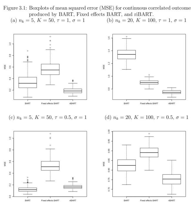
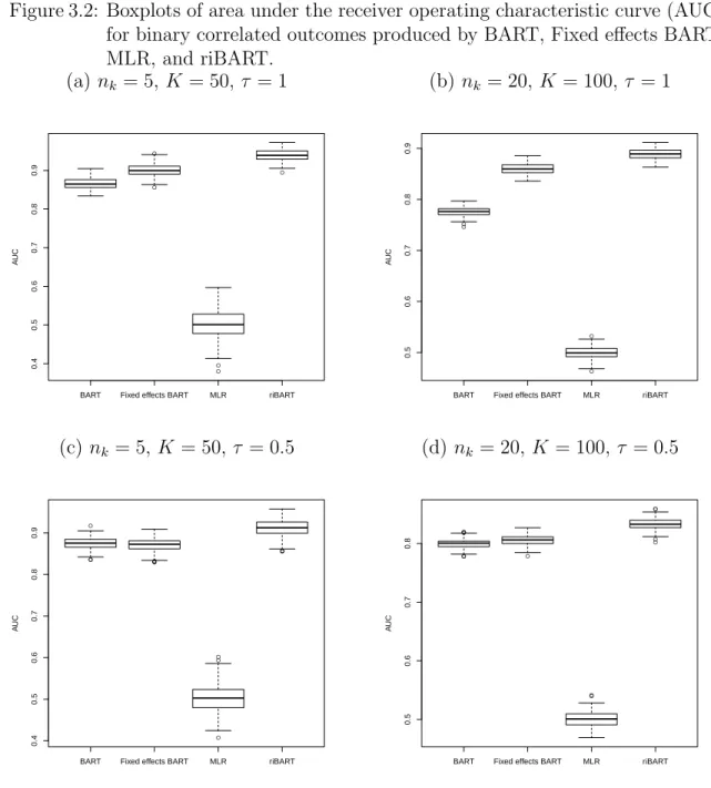
Figure 3.1 shows the boxplots of the MSEs for scenarios 1 to 4 while Figure 3.2 shows the boxplots of the AUCs produced for scenarios 5 to 8. For Figure 3.1, because the boxplots of the MSE for MLR were much larger compared to the rest of the

(51)

methods, these boxplots were not presented in the manuscript. Interested readers may refer to our supplementary materials available online for the graphs including MLR results. For continuous correlated outcomes, riBART produces a clear advantage compared to BART and fixed effects BART when K = 100, nk = 20, and τ = 1. In

other simulation scenarios, riBART does not seem to produce lower MSEs compared to BART and fixed effects BART. For binary correlated outcomes, the advantage of BART in terms of producing a better AUC is more apparent. We observed from Figure 3.2 that riBART produces the higher AUC compared to BART, fixed effects BART, and MLLR in all our simulation scenarios. This suggests that for continuous correlated outcomes, riBART may not yield an obvious prediction advantage except when the values of K, nk, and τ are large. However, for binary correlated outcomes,

riBART would produce an obvious prediction advantage regardless of K, nk, and τ.

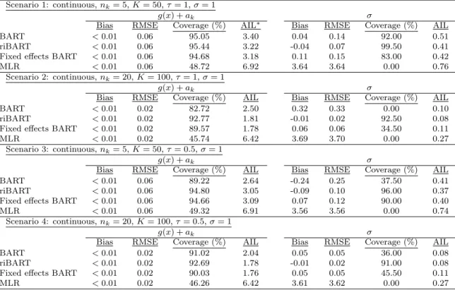
In terms of the inference for the parameters Pm

j=1g(Xik, Tj,Mj) + ak and σ,

Table 3.1 suggests that for continuous correlated outcomes, the bias and RMSE for all methods would be similar under all scenarios forg(x) +ak. However, the coverage

for riBART would be closer to the nominal coverage of 95% under all scenarios. For

σ, the bias produced by riBART was usually the smallest and coverage was usually the highest. These results suggest that riBART should be employed for continuous correlated outcomes if inference for Pm

j=1g(Xik, Tj,Mj) +ak or σ are desired. For

binary correlated outcomes, the main focus of our paper, Table 3.2 suggests that riBART usually has the smallest bias compared with BART, fixed effects BART, and MLLR under all simulation scenarios. riBART also has the better coverage in our simulation scenario compared to the rest of the methods we considered. These results together with the AUC results from Figure 3.2 suggest that for binary correlated outcomes, riBART should be employed.

(52)

Figure 3.1: Boxplots of mean squared error (MSE) for continuous correlated outcomes produced by BART, Fixed effects BART, and riBART.

(a) nk = 5, K = 50, τ = 1, σ = 1 (b) nk= 20, K = 100, τ = 1, σ= 1 ● ● ● ● ● ● ● ● ● ● ● ● ● ● ● ● ●

BART Fixed effects BART riBART

0.2 0.4 0.6 0.8 1.0 MSE ● ●

0.8 1.0 1.2 1.4 1.6 MSE (c) nk = 5, K = 50, τ = 0.5,σ = 1 (d) nk= 20, K = 100,τ = 0.5, σ= 1 ● ● ● ● ● ● ● ● ● ● ● ● ● ● ● ●

0.0 0.2 0.4 0.6 0.8 1.0 MSE ●

0.70 0.75 0.80 0.85 0.90 0.95 1.00 MSE

Novel Applications and Extensions for Bayesian Additive Regression Trees (BART) in Prediction, Imputation, and Causal Inference